Multiobjective approach to optimal control for a tuberculosis model

Abstract

Mathematical modelling can help to explain the nature and dynamics of infection transmissions, as well as support a policy for implementing those strategies that are most likely to bring public health and economic benefits. The paper addresses the application of optimal control strategies in a tuberculosis model. The model consists of a system of ordinary differential equations, which considers reinfection and post-exposure interventions. We propose a multiobjective optimization approach to find optimal control strategies for the minimization of active infectious and persistent latent individuals, as well as the cost associated to the implementation of the control strategies. Optimal control strategies are investigated for different values of the model parameters. The obtained numerical results cover a whole range of the optimal control strategies, providing valuable information about the tuberculosis dynamics and showing the usefulness of the proposed approach.

2010 Mathematics Subject Classification: 90C29; 49N90.

1 Introduction

Tuberculosis (TB) is an important international public health issue. Mycobacterium tuberculosis is a pathogenic bacterial species that is the cause of most occurrences of tuberculosis. It is spread through the air when people who have an active TB infection cough, sneeze, or transmit respiratory fluids through the air. It typically affects the lungs (pulmonary TB) but can affect other sites as well (extrapulmonary TB). The classic symptoms of active TB infection are a chronic cough with blood-tinged sputum, fever, night sweats, and weight loss. Infection of other organs causes a wide range of symptoms. Only approximately 10% of people infected with mycobacterium tuberculosis develop active TB disease, whereas approximately 90% of infected people remain latent. Latent infected TB people are asymptomatic and do not transmit TB, but may progress to active TB through either endogenous reactivation or exogenous reinfection [30, 31]. Treatment of TB depends on close cooperation between patients and health care providers. One can distinguish three types of TB treatment: (i) vaccination to prevent infection; (ii) treatment to cure active TB; (iii) treatment of latent TB to prevent endogenous reactivation [1, 13]. The treatment of active infectious individuals can have different timings [20]. Here we consider treatment with the duration of six months [27]. One of the difficulties related to the success of these treatments is to make sure that patients complete them. After two months, patients no longer have symptoms of the disease and feel healed, so many of them stop taking the medicines. When the treatment is not concluded, the patients are not cured and reactivation can occur and/or the patients may develop resistant TB. One way to prevent patients of not completing the treatment is based on supervision and patient support. This is one of the measures proposed by the Direct Observation Therapy (DOT) of World Health Organization (WHO) [34]. One example of treatment supervision consists in recording each dose of anti-TB drugs on the patients treatment card [34]. These measures are very expensive since the patients need to stay longer in a hospital or specialized people are to be payed to supervise patients till they finish their treatment. On the other hand, it is recognized that the treatment of latent TB individuals reduces the chances of reactivation [13].

Although the anti-TB drugs developed since 1940 have dramatically reduced mortality rates (in clinical cases, cure rates of 90% have been documented) [35], TB remains a major health problem. In 2012, there were 8.6 million of new TB cases and 1.3 million of TB deaths. TB is the second leading cause of death from an infectious disease worldwide after HIV [35]. Mortality rates are especially high without treatment.

Optimal control theory is a branch of mathematics developed to find optimal ways to control a dynamic system [7, 12, 24]. Nowadays, the usefulness of optimal control theory in epidemiology is well recognized [19, 21, 25, 26]. Although different optimal control problems have been recently proposed and applied to TB [4, 10, 15], results in tuberculosis are scarce [17] especially those where optimal strategies are found with respect to different conflicting objectives. Our goal is to show how multiobjective optimization can be used for finding the optimal control strategies in a tuberculosis model. Despite the clear multiobjective nature of the underlying problem, it has been only solved in the past using single-objective approaches. Our main contributions are: (i) to show how to generate the whole range of the optimal strategies, (ii) to provide the analysis of the obtained results with clear advantages with respect to available results in the literature, and (iii) to promote multiobjective optimization in epidemiology.

The paper [17] studies a mathematical model for TB based on [6], considering two classes of infected and latent individuals (infected with typical TB and with resistant strain TB). The authors seek to reduce the number of infected and latent individuals with resistant TB. In [10], the model considers the existence of a class called the lost to follow up individuals and they propose optimal control strategies for the reduction of the number of individuals in this class. In [15], the authors adapt a model from [11] where exogenous reinfection is considered and wish to minimize the number of infectious individuals. In [4], a TB model that incorporates exogenous reinfection, chemoprophylaxis of latently infected individuals and treatment of infections is proposed. Optimal control strategies based on chemoprophylaxis of latently infected individuals and treatment of infectious individuals are analyzed for the reduction of the number of active infected individuals. A TB model, which considers reinfection and post-exposure interventions, was proposed in [13]. The importance of considering reinfection and post-exposure interventions was previously justified in [2, 5, 33]. In [28, 29], a TB model from [13] is extended by adding two controls and two real parameters associated with controls. Optimal strategies are found by minimizing a cost functional that includes the number of active TB infectious and persistent latent individuals as well as the cost of the measures for treatments. An overview of existing TB modelling studies is presented in [16] (see also [8]). These works also identify high-priority areas and challenges for future modelling efforts, which are: (i) the difficult diagnosis and high mortality of TB-HIV; (ii) the high risk of disease progression; (iii) TB health systems in high HIV prevalence settings; (iv) uncertainty in the natural progression of TB-HIV; and (v) combined interventions for TB-HIV.

In this paper we use the model suggested in [29] and propose a multiobjective approach to find optimal control strategies. This approach reflects the intrinsic nature of an underlying decision-making problem. It avoids the use of additional parameters needed to formulate the cost functional and allows to obtain the whole range of optimal solutions. We also investigate the effect of different model parameters. Section 2 presents the mathematical model for tuberculosis with controls. The optimal control problem is then formulated in Section 3, while in Section 4 we present and discuss optimal control strategies obtained by numerical simulations, considering several variations of some of the model parameters. Section 5 compares our approach to find the optimal control strategies, based on the $\epsilon$-constraint method, with the goal attainment and Chebyshev methods. We end with Section 6 of conclusions and some directions of future work.

2 Tuberculosis model with controls

In the following, we consider a TB model taken from [29]. The model without controls is based on [13] and considers reinfection and post-exposure interventions, consisting of a system of nonlinear ordinary differential equations representing population dynamics. In the model, the population is divided into five categories:

$S(t)$	–	susceptible;
$L_{1}(t)$	–	early latent, i.e., individuals recently infected (less than two years) but
		not infectious;
$I(t)$	–	infected, i.e., individuals who have active tuberculosis and are infectious;
$L_{2}(t)$	–	persistent latent, i.e., individuals who were infected and remain latent;
$R(t)$	–	recovered, i.e., individuals who were previously infected and treated.

It is assumed that at birth all individuals are equally susceptible and differentiate as they experience infection and respective therapy [13]. The total population, $N$, is assumed to be constant, so, $N=S(t)+L_{1}(t)+I(t)+L_{2}(t)+R(t)$. This way, it is assumed that the rates of birth and death, $\mu$, are equal (corresponding to a mean life time of 70 years [13]) and there are no disease-related deaths.

The model includes control variables representing prevention and treatment measures, which are continuously implemented during a considered period of disease treatment:

$u_{1}(t)$	–	represents the effort that prevents the failure of treatment in active
		TB infectious individuals, $I$, e.g., supervising the patients, helping them
		to take the TB medications regularly and to complete the TB treatment;
$u_{2}(t)$	–	represents the fraction of persistent latent individuals, $L_{2}$, that is identified
		and put under treatment.

According to [29], the tuberculosis is modeled by the nonlinear time-varying state equations

$$\small\begin{cases}\dot{S}(t)=\mu N-\frac{\beta}{N}I(t)S(t)-\mu S(t)\\ \dot{L_{1}}(t)=\frac{\beta}{N}I(t)\left(S(t)+\sigma L_{2}(t)+\sigma_{R}R(t)\right)-(\delta+\tau_{1}+\mu)L_{1}(t)\\ \dot{I}(t)=\phi\delta L_{1}(t)+\omega L_{2}(t)+\omega_{R}R(t)-(\tau_{0}+\epsilon_{1}u_{1}(t)+\mu)I(t)\\ \dot{L_{2}}(t)=(1-\phi)\delta L_{1}(t)-\sigma\frac{\beta}{N}I(t)L_{2}(t)-(\omega+\epsilon_{2}u_{2}(t)+\tau_{2}+\mu)L_{2}(t)\\ \dot{R}(t)=(\tau_{0}+\epsilon_{1}u_{1}(t))I(t)+\tau_{1}L_{1}(t)+\left(\tau_{2}+\epsilon_{2}u_{2}(t)\right)L_{2}(t)-\sigma_{R}\frac{\beta}{N}I(t)R(t)-\left(\omega_{R}+\mu\right)R(t)\end{cases}$$ (1)

with the initial conditions

$$S(0)=\frac{76}{120}N,\quad L_{1}(0)=\frac{37}{120}N,\quad I(0)=\frac{4}{120}N,\quad L_{2}(0)=\frac{2}{120}N,\quad R(0)=\frac{1}{120}N.$$ (2)

Symbol	Description	Value
$\beta$	Transmission coefficient	$75,100,150,175$
$\mu$	Death and birth rate	$1/70\,yr^{-1}$
$\delta$	Rate at which individuals leave $L_{1}$	$12\,yr^{-1}$
$\phi$	Proportion of individuals going to $I$	$0.05$
$\omega$	Rate of endogenous reactivation for persistent latent infections	$0.0002\,yr^{-1}$
$\omega_{R}$	Rate of endogenous reactivation for treated individuals	$0.00002\,yr^{-1}$
$\sigma$	Factor reducing the risk of infection as a result of acquired
	immunity to a previous infection for $L_{2}$	$0.25$
$\sigma_{R}$	Rate of exogenous reinfection of treated patients	0.25
$\tau_{0}$	Rate of recovery under treatment of active TB	$2\,yr^{-1}$
$\tau_{1}$	Rate of recovery under treatment of latent individuals $L_{1}$	$2\,yr^{-1}$
$\tau_{2}$	Rate of recovery under treatment of latent individuals $L_{2}$	$1\,yr^{-1}$
$N$	Total population	$30000,40000,60000$
$\epsilon_{1}$	Efficacy of treatment of active TB $I$	$0.25,0.5,0.75$
$\epsilon_{2}$	Efficacy of treatment of latent TB $L_{2}$	$0.25,0.5,0.75$
$T$	Total simulation duration	$5\,yr$

Table 1: Model parameters.

The values of the model parameters presented in the control system (1) are given in Table 1. The values of the rates $\delta$, $\phi$, $\omega$, $\omega_{R}$, $\sigma$ and $\tau_{0}$ are taken from [13] and the references cited therein. The parameter $\delta$ denotes the rate at which individuals leave $L_{1}$ compartment; $\phi$ is the proportion of individuals going to compartment $I$; $\omega$ is the rate of endogenous reactivation for persistent latent infections (untreated latent infections); $\omega_{R}$ is the rate of endogenous reactivation for treated individuals (for those who have undergone a therapeutic intervention). The parameter $\sigma$ is the factor that reduces the risk of infection, as a result of acquired immunity to a previous infection, for persistent latent individuals, i.e., this factor affects the rate of exogenous reinfection of untreated individuals; while $\sigma_{R}$ represents the same parameter factor but for treated patients.

The parameter $\tau_{0}$ is the rate of recovery under treatment of active TB, assuming an average duration of infectiousness of six months. The parameters $\tau_{1}$ and $\tau_{2}$ apply to latent individuals $L_{1}$ and $L_{2}$, respectively. They are the rates at which chemotherapy or a post-exposure vaccine is applied [1]. We consider that the rate of recovery of early latent individuals under post-exposure interventions, $\tau_{1}$, is equal to the rate of recovery under treatment of active TB, $\tau_{0}$, and greater than the rate of recovery of persistent latent individuals under post-exposure interventions, $\tau_{2}$.

The parameters $\epsilon_{i}\in(0,1)$, $i=1,2$, measure the effectiveness of the controls $u_{i}$, $i=1,2$, respectively, i.e., these parameters measure the efficacy of treatment interventions for active and persistent latent TB individuals, respectively.

According to [32], the risk of developing disease after infection is much higher in the first five years following infection, and decline exponentially after that. Therefore, as done in [29], we consider here the total simulation duration of $T=5$.

3 Problem formulation

The main goal of our study is to find the most effective ways of applying the controls in (1), aimed at restriction of the tuberculosis epidemic. In this section, we present two formulations of an optimal control problem: (i) the first one, based on optimal control theory; (ii) the second one, based on multiobjective optimization.

3.1 Optimal control problem

The aim is to find the optimal values $u_{1}^{*}$ and $u_{2}^{*}$ of the controls $u_{1}$ and $u_{2}$, such that the associated state trajectories $S^{*}$, $L_{1}^{*}$, $I^{*}$, $L_{2}^{*}$, $R^{*}$ are solution of the system (1) in the time interval $[0,T]$, with initial conditions (2), and minimize an objective functional. Here the objective functional considers the number of active TB infectious individuals $I$, the number of persistent latent individuals $L_{2}$, and the implementation cost of the strategies associated to the controls $u_{i}$, $i=1,2$. The controls are bounded between $0$ and $1$. When the controls vanish, no extra measures are implemented for the reduction of $I$ and $L_{2}$; when the controls take the maximum value $1$, the magnitude of the implemented measures, associated to $u_{1}$ and $u_{2}$, take the value of the effectiveness of the controls, $\epsilon_{1}$ and $\epsilon_{2}$, respectively.

Consider the state system of ordinary differential equations (1) and the set of admissible control functions given by

$$\Omega=\{(u_{1}(\cdot),u_{2}(\cdot))\in(L^{\infty}(0,T))^{2}\,|\,0\leq u_{1}(t),u_{2}(t)\leq 1,\forall t\in[0,T]\}.$$

The objective functional is defined by

$$J(u_{1}(\cdot),u_{2}(\cdot))=\int_{0}^{T}\left[I(t)+L_{2}(t)+W_{1}u_{1}^{2}(t)+W_{2}u_{2}^{2}(t)\right]dt,$$ (3)

where the constants $W_{1}$ and $W_{2}$ are a measure of the relative cost of the interventions associated to the controls $u_{1}$ and $u_{2}$, respectively. We consider the optimal control problem of determining $\left(S^{*}(\cdot),L_{1}^{*}(\cdot),I^{*}(\cdot),L_{2}^{*}(\cdot),R^{*}(\cdot)\right)$, associated to an admissible control pair $\left(u_{1}^{*}(\cdot),u_{2}^{*}(\cdot)\right)\in\Omega$ on the time interval $[0,T]$, satisfying (1), the initial conditions (2), and minimizing the cost function (3), i.e.,

$$J(u_{1}^{*}(\cdot),u_{2}^{*}(\cdot))=\min_{\Omega}J(u_{1}(\cdot),u_{2}(\cdot))\,.$$

3.2 Multiobjective optimization

Without loss of generality, a multiobjective optimization problem with $m$ objectives and $n$ decision variables can be formulated as follows:

$$\begin{array}[]{rl}\text{minimize:}&\boldsymbol{f}(\boldsymbol{x})=(f_{1}(\boldsymbol{x}),f_{2}(\boldsymbol{x}),\ldots,f_{m}(\boldsymbol{x}))^{\text{T}}\\ \text{subject to:}&\boldsymbol{x}\in\Omega,\end{array}$$ (4)

where $\boldsymbol{x}$ is the decision vector, $\Omega\subseteq\mathbb{R}^{n}$ is the feasible decision space, and $\boldsymbol{f}(\boldsymbol{x})$ is the objective vector defined in the objective space $\mathbb{R}^{m}$.

When several objectives are simultaneously optimized, there is no natural ordering in the objective space. The objective space is partially ordered. In such a scenario, solutions are compared on the basis of the Pareto dominance relation.

Definition 3.2.1 (Pareto dominance).

For two solutions $\boldsymbol{a}$ and $\boldsymbol{b}$ from $\Omega$, a solution $\boldsymbol{a}$ is said to dominate a solution $\boldsymbol{b}$ (denoted by $\boldsymbol{a}\prec\boldsymbol{b}$) if

$$\forall i\in\{1,\ldots,m\}:f_{i}(\boldsymbol{a})\leq f_{i}(\boldsymbol{b})\,\wedge\,\exists j\in\{1,\ldots,m\}:f_{j}(\boldsymbol{a})<f_{j}(\boldsymbol{b}).$$

The presence of multiple conflicting objectives gives rise to a set of optimal solutions, generally known as the Pareto optimal set. The concepts of optimality for multiobjective optimization are defined as follows.

Definition 3.2.2 (Pareto optimality).

A solution $\boldsymbol{x}^{\ast}\in\Omega$ is Pareto optimal if and only if

$$\nexists\boldsymbol{y}\in\Omega:\boldsymbol{y}\prec\boldsymbol{x}^{\ast}.$$

Definition 3.2.3 (Pareto optimal set).

For a multiobjective optimization problem (4), the Pareto optimal set (or Pareto set, for short) is defined as

$$\mathcal{PS}^{\ast}=\{\boldsymbol{x}^{\ast}\in\Omega\,|\,\nexists\boldsymbol{y}\in\Omega:\boldsymbol{y}\prec\boldsymbol{x}^{\ast}\}.$$

Definition 3.2.4 (Pareto optimal front).

For a multiobjective optimization problem (4) and the Pareto optimal set $\mathcal{PS}^{\ast}$, the Pareto optimal front (or Pareto front, for short) is defined as

$$\mathcal{PF}^{\ast}=\{\boldsymbol{f}(\boldsymbol{x}^{\ast})\in\mathbb{R}^{m}\,|\,\boldsymbol{x}^{\ast}\in\mathcal{PS}^{\ast}\}.$$

3.3 Proposed approach

An approach based on optimal control theory allows to obtain a single optimal solution for the cost functional (3), which is defined from some decision maker’s perspective using the constants $W_{1}$ and $W_{2}$. The most straightforward disadvantage is that only a limited amount of information about the choice of the optimal strategy can be presented to the decision maker. Moreover, the choice of proper values of $W_{1}$ and $W_{2}$ is not straightforward, generally being not an easy task.

In our approach, we decompose the cost functional shown in (3) into two components representing different aspects taken into consideration when dealing with tuberculosis. Then, we use a multiobjective optimization method to simultaneously optimize the defined objectives. Thus, the multiobjective optimization problem is defined as:

$$\begin{array}[]{rl}\text{minimize}&f_{1}(u_{1}(\cdot),u_{2}(\cdot))=\displaystyle\int_{0}^{T}\left[I(t)+L_{2}(t)\right]dt,\\[5.69046pt] &f_{2}(u_{1}(\cdot),u_{2}(\cdot))=\displaystyle\int_{0}^{T}\left[u_{1}^{2}(t)+u_{2}^{2}(t)\right]dt,\end{array}$$ (5)

where $f_{1}$ represents the number of active infected and latent individuals, and $f_{2}$ represents the cost associated to the implementation of the control policies.

4 Numerical experiments

We now present and discuss the numerical results for the optimal controls using the multiobjective optimization approach. We also investigate the effects of different parameters values on the optimal control strategies and dynamics of the tuberculosis model.

4.1 $\epsilon$-Constraint method

The $\epsilon$-constraint method was introduced in [14]. In this method, one of the objective functions is selected to be minimized, whereas all the other functions are converted into constrains by setting an upper bound to each of them. The problem to be solved is of the following form:

$$\begin{array}[]{rlll}\underset{\boldsymbol{x}\in\Omega}{\text{minimize:}}&f_{l}(\boldsymbol{x})&\\ \text{subject to:}&f_{i}(\boldsymbol{x})\leq\epsilon_{i},&\forall i\in\{1,\ldots,m\}\wedge i\neq l.\end{array}$$ (6)

In the above formulation, the $l$th objective is minimized, and the parameter $\epsilon_{i}$ represents an upper bound of the value of $f_{i}$. The $\epsilon$-constraint method is able to obtain solutions in convex and nonconvex regions of the Pareto optimal front. When all the objective functions in the problem (4) are convex, as it happens in our study, the problem (6) is also convex and it has a unique solution. The unique solution of the problem (6) is Pareto optimal for any given upper bound vector $\boldsymbol{\epsilon}=\{\epsilon_{1},\ldots,\epsilon_{m-1}\}$. For a proof see [23].

4.2 Experimental setup

The system (1) is numerically integrated using the fourth-order Runge–Kutta method. The controls are discretized using $60$ equally spaced time intervals over the period of $[0,T]$. The integrals in (5) are calculated using the trapezoidal rule. Using the formulation (6), we minimize the first objective in (5) setting $f_{2}$ as the constraint bounded by the values of $\epsilon$, which are selected by dividing the range of $f_{2}$ into 100 evenly distributed intervals. The range of $f_{2}$ is calculated as $f_{2}^{\min}=0$ for $u_{1}(\cdot),u_{2}(\cdot)\equiv 0$ and $f_{2}^{\max}=10$ for $u_{1}(\cdot),u_{2}(\cdot)\equiv 1$. To solve the problems with different $\epsilon$, we use the MATLAB^® built-in function fmincon with a sequential quadratic programming algorithm, setting the maximum number of function evaluations to $20,000$.

4.3 Experimental results

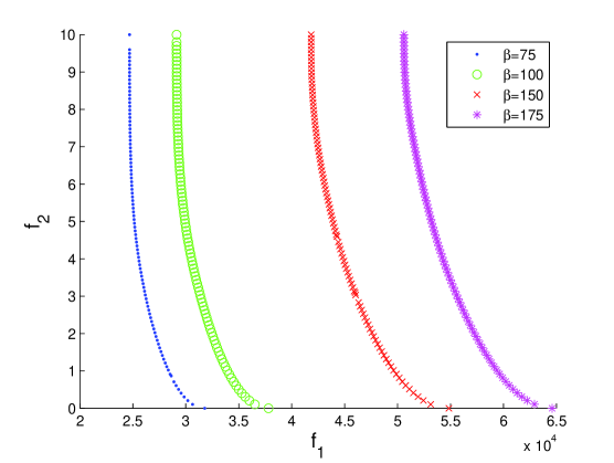
Figure 1: Trade-off curves for different values of $\beta$.

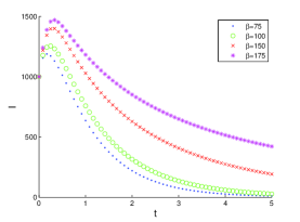
(a) $I$ for $f_{2}=0$

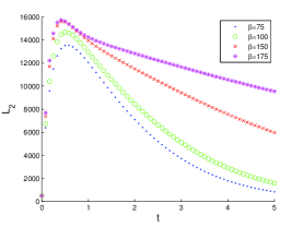
(b) $L_{2}$ for $f_{2}=0$

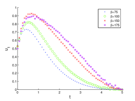
(c) $u_{1}$ for $f_{2}=2.5$

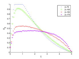
(d) $u_{2}$ for $f_{2}=2.5$

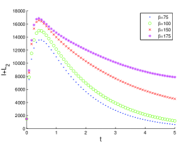
(e) $I+L_{2}$ for $f_{2}=2.5$

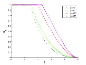
(f) $u_{1}$ for $f_{2}=5$

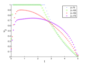
(g) $u_{2}$ for $f_{2}=5$

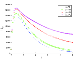
(h) $I+L_{2}$ for $f_{2}=5$

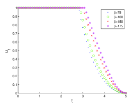
(i) $u_{1}$ for $f_{2}=7.5$

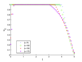
(j) $u_{2}$ for $f_{2}=7.5$

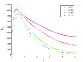
(k) $I+L_{2}$ for $f_{2}=7.5$

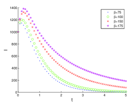
(l) $I$ for $f_{2}=10$

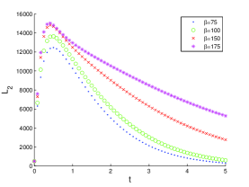
(m) $L_{2}$ for $f_{2}=10$

Figure 2: Changes of controls, infectious and persistent latent individuals for different values of $\beta$.

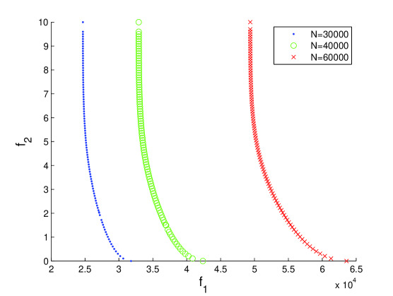
Figure 3: Trade-off curves for different values of $N$.

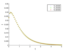
(a) $I/N$ for $f_{2}=0$

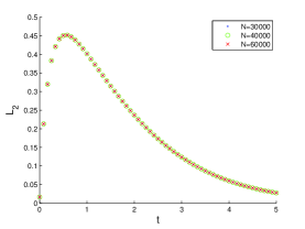
(b) $L_{2}/N$ for $f_{2}=0$

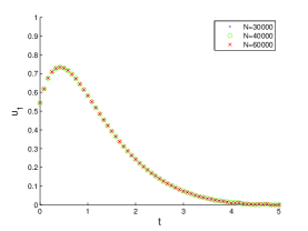
(c) $u_{1}$ for $f_{2}=2.5$

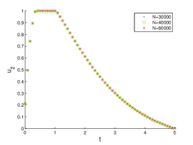
(d) $u_{2}$ for $f_{2}=2.5$

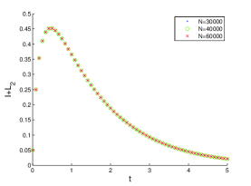
(e) $(I+L_{2})/N$ for $f_{2}=2.5$

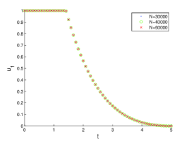
(f) $u_{1}$ for $f_{2}=5$

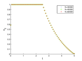
(g) $u_{2}$ for $f_{2}=5$

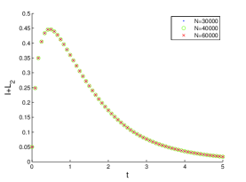
(h) $(I+L_{2})/N$ for $f_{2}=5$

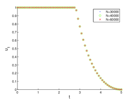
(i) $u_{1}$ for $f_{2}=7.5$

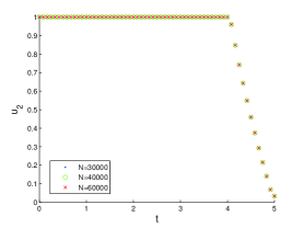
(j) $u_{2}$ for $f_{2}=7.5$

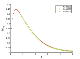
(k) $(I+L_{2})/N$ for $f_{2}=7.5$

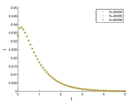
(l) $I/N$ for $f_{2}=10$

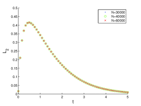
(m) $L_{2}/N$ for $f_{2}=10$

Figure 4: Changes of controls, infectious and persistent latent individuals for different values of $N$.

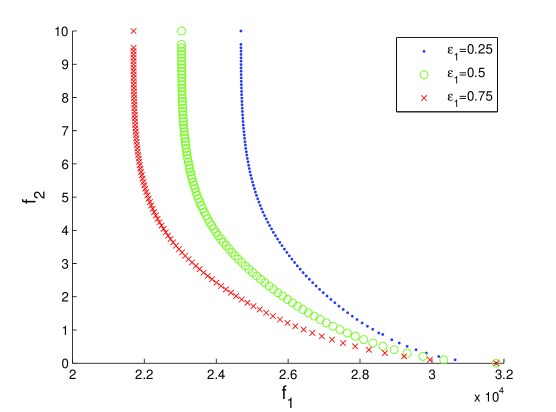
Figure 5: Trade-off curves for different values of $\epsilon_{1}$.

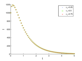
(a) $I$ for $f_{2}=0$

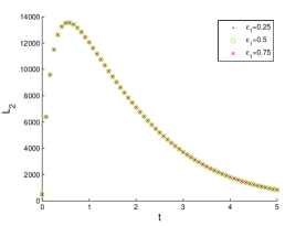
(b) $L_{2}$ for $f_{2}=0$

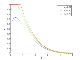
(c) $u_{1}$ for $f_{2}=2.5$

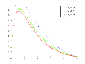
(d) $u_{2}$ for $f_{2}=2.5$

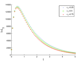
(e) $I+L_{2}$ for $f_{2}=2.5$

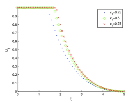
(f) $u_{1}$ for $f_{2}=5$

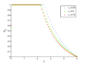
(g) $u_{2}$ for $f_{2}=5$

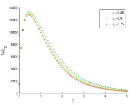
(h) $I+L_{2}$ for $f_{2}=5$

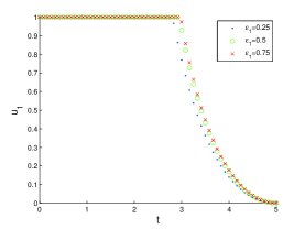
(i) $u_{1}$ for $f_{2}=7.5$

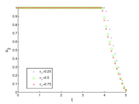
(j) $u_{2}$ for $f_{2}=7.5$

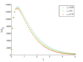
(k) $I+L_{2}$ for $f_{2}=7.5$

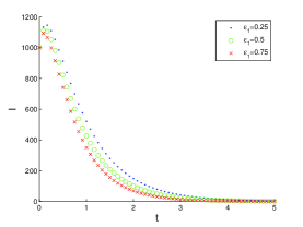
(l) $I$ for $f_{2}=10$

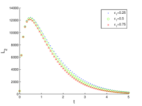
(m) $L_{2}$ for $f_{2}=10$

Figure 6: Changes of controls, infectious and persistent latent individuals for different values of $\epsilon_{1}$.

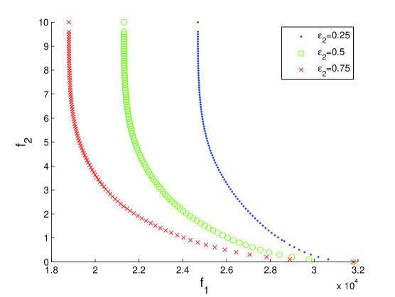
Figure 7: Trade-off curves for different values of $\epsilon_{2}$.

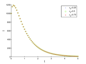
(a) $I$ for $f_{2}=0$

(b) $L_{2}$ for $f_{2}=0$

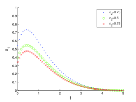
(c) $u_{1}$ for $f_{2}=2.5$

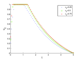
(d) $u_{2}$ for $f_{2}=2.5$

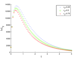
(e) $I+L_{2}$ for $f_{2}=2.5$

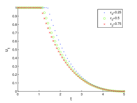
(f) $u_{1}$ for $f_{2}=5$

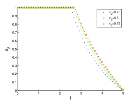
(g) $u_{2}$ for $f_{2}=5$

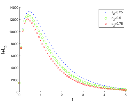
(h) $I+L_{2}$ for $f_{2}=5$

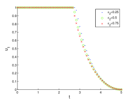
(i) $u_{1}$ for $f_{2}=7.5$

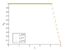
(j) $u_{2}$ for $f_{2}=7.5$

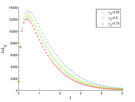
(k) $I+L_{2}$ for $f_{2}=7.5$

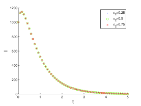
(l) $I$ for $f_{2}=10$

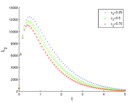
(m) $L_{2}$ for $f_{2}=10$

Figure 8: Changes of controls, infectious and persistent latent individuals for different values of $\beta$.

In the following, we discuss the obtained optimal solutions to the problem (5), considering the variations of some model parameters separately. Since there is a set of optimal solutions to the problem (5), considering all the solutions is somewhat cumbersome, and we divide the obtained trade-off solutions into different parts, selecting a representative solution to each part for analysis. For this purpose, we consider five cases: $f_{2}=0$, $f_{2}=2.5$, $f_{2}=5$, $f_{2}=7.5$, and $f_{2}=10$. Each case represents an amount of available resources for treatment. For each case, the best solution with respect to $f_{1}$ in the corresponding set of trade-off solutions is considered. In particular, the first case ($f_{2}=0$) represents the situation without controls ($u_{1}(\cdot),u_{2}(\cdot)\equiv 0$), reflecting the economical perspective. The last case ($f_{2}=10$) represents the situation where the maximum controls are applied ($u_{1}(\cdot),u_{2}(\cdot)\equiv 1$), being the most preferable scenario from medical perspective. Whereas three other cases ($f_{2}=2.5$, $f_{2}=5$, $f_{2}=7.5$) represent intermediate scenarios, providing trade-offs between the number of affected by the tuberculosis and expenses for treatment.

Figure 1 plots the trade-off solutions obtained for four different values of the transition coefficient, $\beta$. From the figure, it can be seen that the higher $\beta$ the higher number of infectious and persistent latent individuals is. Also, the difference between the worst and the best case scenarios from medical perspective becomes larger, if $\beta$ is increased.

Figure 2 shows the changes of the number of infectious and persistent latent individuals, as well as the controls, for solutions in different parts of the trade-off curves with varying $\beta$. Figures 2(a) and 2(b) show the changes of $I$ and $L_{2}$, respectively, without the controls ($f_{2}=0$). On the other hand, Figures 2(l) and 2(m) illustrate the case where the maximum controls are applied ($u_{1}(\cdot),u_{2}(\cdot)\equiv 1$). From these figures and Figures 2(e), 2(h) and 2(k), it can be seen that if $\beta$ increases, then the number of infectious and persistent latent individuals grows. From Figures 2(c), 2(f) and 2(i), one can see that $u_{1}$ is usually larger for higher values of $\beta$. However, Figures 2(d), 2(g) and 2(j) suggest that optimal values of $u_{2}$ are not always larger for higher values of $\beta$. Thus, with an increasing of $\beta$, more effort must be put on the prevention of failure of treatment in active infectious individuals. Moreover, the fraction of individuals that are put under treatment must be decreased during the first part of the period, and increased during the second part of the period when $\beta$ grows.

Figure 3 displays the trade-off solutions obtained for three different population sizes, $N$. We can see that larger population sizes result in the higher numbers of infectious and persistent latent individuals. Also, the range of optimal values of $f_{1}$ grows when $N$ rises.

Figure 4 shows the changes of the controls as well as the fractions of the number of infectious and persistent latent individuals for solutions in different parts of the trade-off curves for different $N$. Although the number of infectious and persistent latent individuals grows for larger $N$, Figures 4(a), 4(b), 4(l) and 4(m) show that the fractions of $I/N$ and $L_{2}/N$ do not vary when $(u_{1}(\cdot),u_{2}(\cdot))\equiv 0$ and $(u_{1}(\cdot),u_{2}(\cdot))\equiv 1$, respectively. Similarly, the fractions $(I+L_{2})/N$ remain unchanged for intermediate solutions when $N$ is varied (Figures 4(e), 4(h) and 4(k)). From the plots for the controls in Figure 4, we can seen that the optimal control strategies do not depend on the population size.

Figure 5 presents the trade-off solutions when the efficacy of treatment of active tuberculosis individuals, $\epsilon_{1}$, is varying. The figure shows that increasing $\epsilon_{1}$ allows to reduce the number of infectious and persistent latent individuals.

The plots for infectious and persistent latent individuals presented in Figure 6 demonstrate that the higher efficacy of treatment of active individuals the lower the number of infectious and persistent latent individuals is. Concerning the controls, Figures 6(c), 6(f) and 6(i) show that the optimal control $u_{1}$ is higher when $\epsilon_{1}$ is increased. On the contrary, the optimal control $u_{2}$ decreases when $\epsilon_{1}$ is increased (Figures 6(d), 6(g) and 6(j)). This suggests that for efficiently reducing $I+L_{2}$ when increasing $\epsilon_{1}$ we must focus on policies associated with $u_{1}$, namely the supervision and the support of active infectious individuals, and decrease the fraction of individuals that are put under treatment.

Figure 7 shows the trade-off solutions when the efficacy of treatment of latent tuberculosis individuals, $\epsilon_{2}$, is varying. Similarly to the case of varying $\epsilon_{1}$ shown in Figure 5, this figure suggests that increasing $\epsilon_{2}$ allows to reduce the number of infectious and persistent latent individuals. Though, the larger decrease in $I+L_{2}$ can be achieved by increasing $\epsilon_{2}$ compared to the same values of $\epsilon_{1}$.

Figures 8(l) and 8(m) show that by implementing the maximum controls, $I$ has the same values for different $\epsilon_{2}$, whereas $L_{2}$ decreases when $\epsilon_{2}$ is increased. Also, $I+L_{2}$ becomes smaller when $\epsilon_{2}$ increases, as it can be seen analyzing intermediate trade-off solutions in Figures 8(e), 8(h) and 8(k). The plots for the controls presented in Figure 8 show that $u_{1}$ becomes smaller when $\epsilon_{2}$ increases, whereas $u_{2}$ grows when $\epsilon_{2}$ is increased. This suggest that, to efficiently reduce $I+L_{2}$ with increasing $\epsilon_{2}$, we must focus on implementation of $u_{2}$, which is related to the fraction of persistent latent individuals that is put under treatment.

5 Methods Comparison

In this section, we compare our approach to find the optimal control strategies in a tuberculosis model, based on the $\epsilon$-constraint method (Section 4), with two other scalarization methods for solving multiobjective optimization problems. The first one is based on the goal attainment method, which was applied for solving multiobjective control problems in some recent studies [18, 22]. Another popular method is based on Chebyshev problem (or Chebyshev method). Follows the description of the two methods.

5.1 Goal attainment method

The goal attainment method [23] reformulates the problem shown in (4) as folows:

$$\left\{\begin{array}[]{rl}\underset{\boldsymbol{x}\in\Omega,\alpha\geq 0}{\text{minimize:}}&\alpha\\ \text{subject to:}&w_{1}(f_{1}(\boldsymbol{x})-z^{\ast}_{1})\leq\alpha\\ &\qquad\vdots\\ &w_{m}(f_{m}(\boldsymbol{x})-z^{\ast}_{m})\leq\alpha,\\ \end{array}\right.$$ (7)

where $\boldsymbol{z}^{\ast}=(z^{\ast}_{1},\ldots,z^{\ast}_{m})^{\text{T}}$ is a reference point, $\boldsymbol{w}=(w_{1},\ldots,w_{m})^{\text{T}}$ is a weight vector ($\sum\limits_{j=1}\limits^{m}w_{j}=1$), and $\boldsymbol{x}\in\Omega,\alpha\in\mathbb{R}_{+}$ are variables. Solving the above problem for different weight vectors allows to obtain multiple Pareto optimal solutions. In [9] the problem (7) is referred to as Pascoletti–Serafini scalarization.

5.2 Chebyshev method

The Chebyshev method belongs to the class of weighted metric methods [23], which minimize the distance between some reference point and the feasible objective region. The weighted metric methods use the weighted $L_{p}$ metrics for measuring the distance from any solution to the reference point. Chebyshev method is referred to the case with $p=\infty$, which can be formulated as

$$\underset{\boldsymbol{x}\in\Omega}{\text{minimize:}}\max\limits_{1\leq i\leq m}\,\{w_{i}(f_{i}(\boldsymbol{x})-z^{\ast}_{i})\},$$ (8)

where $\boldsymbol{z}^{\ast}=(z^{\ast}_{1},\ldots,z^{\ast}_{m})^{\text{T}}$ is a reference point, and $\boldsymbol{w}=(w_{1},\ldots,w_{m})^{\text{T}}$ is a weight vector ($\sum\limits_{j=1}\limits^{m}w_{j}=1$). Similarly to the goal attainment method, for finding multiple Pareto optimal solutions the problem (8) must be solved for different weight vectors. The problem shown in (8) was originally introduced in Bowman [3]. In the literature, the name of the method may vary due to different ways of spelling.

5.3 Results

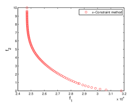
(a) $\epsilon$-Constraint method

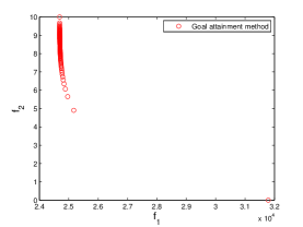
(b) Goal attainment method

(c) Chebyshev method

Figure 9: Trade-off curves obtained by different methods.

For a set of 100 uniformly distributed weight vectors, each method was executed on the tuberculosis model, having the remaining settings as in Section 4.2. Figure 9 plots trade-off solutions obtained afterwards, including the $\epsilon$-constraint method. As it is seen, the $\epsilon$-constraint method produces a well-distributed set of trade-of solutions, whereas the solutions obtained by the other methods do not cover the whole Pareto optimal region. This is because the objective functions are differently scaled. The use of scalarization schemes based on the weight vectors makes the goal attainment method and Chebyshev method sensitive to the scale of objectives, resulting in significant performance deterioration, in terms of the uniformness of obtained solutions, in the case of disparately scaled objectives. On the other hand, the $\epsilon$-constraint method divides the Pareto region into a number of subregions with respect to the values of $\epsilon$, minimizing the chosen objective. In this case, the relative scale of objectives does not matter significatively, with the approach being able to locate solutions in all parts of the Pareto optimal region.

To quantitatively compare the outcomes of the three methods, we rely on the hypervolume [36], which has been utilized extensively for the comparison of multiobjective algorithms. The hypervolume uses the volume of the dominated portion of the objective space as a measure for the quality. Table 2 shows the hypervolume values for the three methods, which are computed after normalizing the objective values of the obtained solutions and using the nadir point as a reference point. The results summarized in Table 2 confirm our previous observation, with the $\epsilon$-constraint method producing the best results.

	$\epsilon$-Constraint method	Goal attainment method	Chebyshev method
Hypervolume	0.82481	0.50034	0.50031

Table 2: Hypervolume values for trade-off solutions obtained by the three methods (the higher the better).

6 Conclusions

The incidence rates of tuberculosis have been declining since 2004 worldwide. Mortality rates, at global level, fell down around 45% between 1990 and 2012, and if the current rate of decline is sustained, by 2015 the target of a 50% reduction can be achieved. The reduction of mortality and incidence rates is due to prevention and treatment policies that have been applied in the last years.

In this paper we study a mathematical model for tuberculosis from the optimal control point of view, using a multiobjective approach. The optimal control strategies are found by simultaneously minimizing the number of individuals affected by the tuberculosis and the cost of implementation of prevention and treatment policies. This approach avoids the use of additional weight coefficients to formulate a single cost functional and reflects the intrinsic nature of the problem.

The results obtained in this study clearly show that a multiobjective approach is effective to finding optimal control strategies in a mathematical model for tuberculosis. The obtained trade-off solutions reveal different perspectives on the implementation of prevention and treatment policies. Once a set of optimal solutions is calculated, the final decision on the control strategy can be made taking into account the goals of public health care and the available resources for treatment. We also investigate the optimal control strategies with varying model parameters. It is observed that as the transmission coefficient increases, the fraction of active infectious and persistent latent individuals increases as well, corresponding to the case where the disease may become endemic. Varying the population size, the optimal control strategies remain unchanged. Increasing the efficacy of control policies allows to reduce the number of active infectious and persistent latent individuals. When the measure of efficacy for some control is increased, the main focus of efficiently dealing with the disease must be on the policies associated with the corresponding control for which the efficacy is improved.

Finally, we compared the approach proposed in our work with other scalarization techniques for multiobjective optimization. The obtained results show that the $\epsilon$-constraint method is an appropriate choice for finding the optimal control strategies in the tuberculosis model.

As future work, it would be interesting to further investigate different values for the model parameters and observe the variations on the optimal control strategies. We also plan to consider the second objective as an $L^{1}$ functional, with the control variable appearing linearly.

Acknowledgements

Denysiuk would like to thank AdI – Innovation Agency, for the financial support awarded through POFC program, for the R&D project SustIMS – Sustainable Infrastructure Management Systems (FCOMP-01-0202-FEDER-023113) and to ISISE – Institute for Sustainability and Innovation in Structural Engineering (PEst-C/ECI/UI4029/2011 FCOM-01-0124-FEDER-022681). Silva and Torres were supported by Portuguese funds through the Center for Research and Development in Mathematics and Applications (CIDMA), and The Portuguese Foundation for Science and Technology (FCT), within project PEst-OE/MAT/UI4106/2014. Silva is also grateful to the FCT post-doc fellowship SFRH/BPD/72061/2010; Torres to the FCT project PTDC/EEI-AUT/1450/2012, co-financed by FEDER under POFC-QREN with COMPETE reference FCOMP-01-0124-FEDER-028894. The authors would like to thank the Editor and two anonymous referees for valuable comments and suggestions.

References

- [1] L. J. Abu-Raddad, L. Sabatelli, J. T. Achterberg, J. D. Sugimoto, I. M. Longini, C. Dye, and M. E. Halloran, Epidemiological benefits of more-effective tuberculosis vaccines, drugs, and diagnostics, PNAS 106, 33 (2009), pp. 13980–13985.
- [2] A. Bandera, A. Gory, L. Catozzi, A. Degli Esposti, G. Marchetti, C. Molteni, G. Ferrario, L. Codecasa, V. Penati, A. Matteelli, F. Franzetti, Molecular epidemiology study of exogenous reinfection in an area with a low incidence of tuberculosis, J. Clin. Microbiol. 39 (2001), no. 6, pp. 2213–2218.
- [3] V. J. Bowman Jr., On the Relationship of the Chebyshev Norm and the Efficient Frontier of Multiple Criteria Objectives, Lecture Notes in Economics and Mathematical Systems, 130 (1976), pp. 76–86.
- [4] S. Bowong, Optimal control of the transmission dynamics of tuberculosis, Nonlinear Dynam. 61 (2010), no. 4, pp. 729–748.
- [5] J. A. Caminero, M. J. Pena, M. I. Campos-Herrero, J. C. Rodriguez, O. Afonso, C. Martin, J. M. Pavón, M. J. Torres, M. Burgos, P. Cabrera, P. M. Small, D. A. Enarson, Exogenous reinfection with tuberculosis on a European island with a moderate incidence of disease, Am. J. Respir. Crit. Care Med. 163 (2001), no. 3, pp. 717–720.
- [6] C. Castillo-Chavez, Z. Feng, To treat or not to treat: the case of tuberculosis, J. Math. Biol. 35 (1997), no. 6, pp. 629–656.
- [7] L. Cesari, Optimization — Theory and Applications. Problems with Ordinary Differential Equations, Applications of Mathematics 17, Springer-Verlag, New York, 1983.
- [8] T. Cohen, M. Lipsitch, R. P. Walensky, and M. Murray, Beneficial and perverse effects of isoniazid preventive therapy for latent tuberculosis infection in HIV tuberculosis coinfected populations, PNAS 103, 18 (2006), pp. 7042–7047.
- [9] G. Eichfelder, Adaptive Scalarization Methods in Multiobjective Optimization, Springer, Berlin, Heidelberg, 2008.
- [10] Y. Emvudu, R. Demasse, D. Djeudeu, Optimal control of the lost to follow up in a tuberculosis model, Comput. Math. Methods Med. 2011 (2011), Art. ID 398476, 12 pp.
- [11] Z. Feng, C. Castillo-Chavez, A. F. Capurro, A model for tuberculosis with exogenous reinfection, Theor. Pop. Biol. 57 (2000), no. 3, pp. 235–247.
- [12] W. H. Fleming, R. W. Rishel, Deterministic and Stochastic Optimal Control, Springer Verlag, New York, 1975.
- [13] M. G. M. Gomes, P. Rodrigues, F. M. Hilker, N. B. Mantilla-Beniers, M. Muehlen, A. C. Paulo, G. F. Medley, Implications of partial immunity on the prospects for tuberculosis control by post-exposure interventions, J. Theoret. Biol. 248 (2007), no. 4, pp. 608–617.
- [14] Y. Y. Haimes, L. S. Lasdon, and D. A. Wismer, On a bicriterion formulation of the problems of integrated system identification and system optimization, IEEE Transactions on Systems, Man and Cybernetics 1 (1971), pp. 296–297.
- [15] K. Hattaf, M. Rachik, S. Saadi, Y. Tabit, N. Yousfi, Optimal control of tuberculosis with exogenous reinfection, Appl. Math. Sci. (Ruse) 3 (2009), no. 5-8, pp. 231–240.
- [16] R. M. G. J. Houben, D. W. Dowdy, A. Vassall, T. Cohen, M. P. Nicol, R. M. Granich, J. E. Shea, P. Eckhoff, C. Dye, M. E. Kimerling, R. G. White, How can mathematical models advance tuberculosis control in high HIV prevalence settings?, International Journal of Tuberculosis and Lung Disease 18 (2014), no. 5, pp. 509–514.
- [17] E. Jung, S. Lenhart, Z. Feng, Optimal control of treatments in a two-strain tuberculosis model, Discrete Contin. Dyn. Syst. Ser. B 2 (2002), no. 4, pp. 473–482.
- [18] C. Y. Kaya, H. Maurer, A numerical method for nonconvex multi-objective optimal control problems, Comput. Optim. Appl. 57 (2014), no. 3, pp. 685–702.
- [19] Q. Kong, Z. Qiu, Z. Sang, Y. Zou, Optimal control of a vector-host epidemics model, Math. Control Relat. Fields 1 (2011), no. 4, pp. 493–508.
- [20] M. E. Kruk, N. R. Schwalbe, C. A. Aguiar, Timing of default from tuberculosis treatment: a systematic review, Trop. Med. Int. Health 13 (2008), no. 5, pp. 703–712.
- [21] S. Lenhart, J. T. Workman, Optimal control applied to biological models, Chapman & Hall/CRC, Boca Raton, FL, 2007.
- [22] F. Logist, B. Houska, M. Diehl, J. van Impe, Fast Pareto set generation for nonlinear optimal control problems with multiple objectives, Struct. Multidiscip. Optim., 42 (2010), pp. 591–603.
- [23] K. Miettinen, Nonlinear multiobjective optimization, Kluwer Academic Publishers, 1999.
- [24] L. Pontryagin, V. Boltyanskii, R. Gramkrelidze, E. Mischenko, The Mathematical Theory of Optimal Processes, Wiley Interscience, 1962.
- [25] H. S. Rodrigues, M. T. T. Monteiro, D. F. M. Torres, Dynamics of dengue epidemics when using optimal control, Math. Comput. Modelling 52 (2010), no. 9-10, pp. 1667–1673. arXiv:1006.4392
- [26] H. S. Rodrigues, M. T. T. Monteiro, D. F. M. Torres, A. Zinober, Dengue disease, basic reproduction number and control, Int. J. Comput. Math. 89 (2012), no. 3, pp. 334–346. arXiv:1103.1923
- [27] P. Rodrigues, C. J. Silva, D. F. M. Torres, Cost-effectiveness analysis of optimal control measures for tuberculosis, Bull. Math. Biol. 76 (2014), no. 10, 2627–2645. arXiv:1409.3496
- [28] S. J. Silva, D. F. M. Torres, Optimal control strategies for tuberculosis treatment: a case study in Angola, Numer. Algebra Control Optim. 2 (2012), no. 3, pp. 601–617. arXiv:1203.3255
- [29] S. J. Silva, D. F. M. Torres, Optimal control for a tuberculosis model with reinfection and post-exposure interventions, Math. Biosci. 244 (2013), no. 2, pp. 154–164. arXiv:1305.2145
- [30] P. M. Small, P. I. Fujiwara, Management of tuberculosis in the United States, N. Engl. J. Med. 345 (2001), no. 3, pp. 189–200.
- [31] K. Styblo, State of art: epidemiology of tuberculosis, Bull. Int. Union Tuberc. 53 (1978), pp. 141–152.
- [32] K. Styblo, Epidemiology of tuberculosis: epidemiology of tuberculosis in HIV prevalent countries, Royal Netherlands Tuberculosis Association, 1991.
- [33] A. van Rie, R. Warren, M. Richardson, T. C. Victor, R. P. Gie, D. A. Enarson, N. Beyers, P. D. van Helden, Exogeneous reinfection as a cause of recurrent tuberculosis after curative treatment, N. Engl. J. Med. 341 (1999), pp. 1174–1179.
- [34] WHO, Treatment of tuberculosis guidelines, Fourth edition, WHO Report, Geneva, 2010.
- [35] WHO, Global Tuberculosis Control, WHO Report, Geneva, 2012.
- [36] E. Zitzler, L. Thiele, Multiobjective optimization using evolutionary algorithms - A comparative case study. In: Proceedings of the Conference on Parallel Problem Solving From Nature. PPSN’98 (1998), pp. 292–304.