Further Results on Lyapunov-Like Conditions of Forward Invariance and Boundedness for a Class of Unstable Systems

Abstract

We provide several characterizations of convergence to unstable equilibria in nonlinear systems. Our current contribution is three-fold. First we present simple algebraic conditions for establishing local convergence of non-trivial solutions of nonlinear systems to unstable equilibria. The conditions are based on the earlier work [1] and can be viewed as an extension of the Lyapunov’s first method in that they apply to systems in which the corresponding Jacobian has one zero eigenvalue. Second, we show that for a relevant subclass of systems, persistency of excitation of a function of time in the right-hand side of the equations governing dynamics of the system ensure existence of an attractor basin such that solutions passing through this basin in forward time converge to the origin exponentially. Finally we demonstrate that conditions developed in [1] may be remarkably tight.

I Introduction

Analysis of asymptotic behavior of solutions of nonlinear systems is one of the central pillars of modern control theory. Lyapunov stability [2] is an example of such characterizations. The notion of Lyapunov stability and analysis methods that are based on this notion are proven successful in a wide range of engineering applications (see e.g. [3], [4], [5], [6] is a non-exhaustive list of references). The popularity and success of the concept of Lyapunov stability resides, to a substantial degree, in the convenience and utility of the method of Lyapunov functions for assessing asymptotic properties of solutions of ordinary differential equations. Instead of deriving the solutions explicitly it suffices to solve an algebraic inequality involving partial derivatives of a given Lyapunov candidate function. Yet, as the methods of control expand from purely engineering applications into a wider area of science, there is a need for maintaining behavior that fails to obey the usual requirement of Lyapunov stability.

There are numerous examples of systems possessing Lyapunov-unstable, yet attracting, invariant sets [7], e.g., in the domains of aircraft dynamics and design of synchronous generators [8] (pp. 313–356). Other examples include models of decision-making sequences [9], [10], [11], flutter suppressors [12], the general problem of universal adaptive stabilization [13, 14], and problems of adaptive observer design for systems with nonlinear in parameter right-hand side [15]. Finding rigorous, convenient and at the same time tight criteria for asymptotic convergence to Lyapunov-unstable invariant sets, however, is a non-trivial problem.

Criteria for checking attractivity of unstable point attractors in a rather general setting have been proposed in [16], and were further developed in [17, 18]. These results apply to systems in which almost all points in a neighborhood of the attractor correspond to solutions converging to the attractor asymptotically. However, as Figure 1

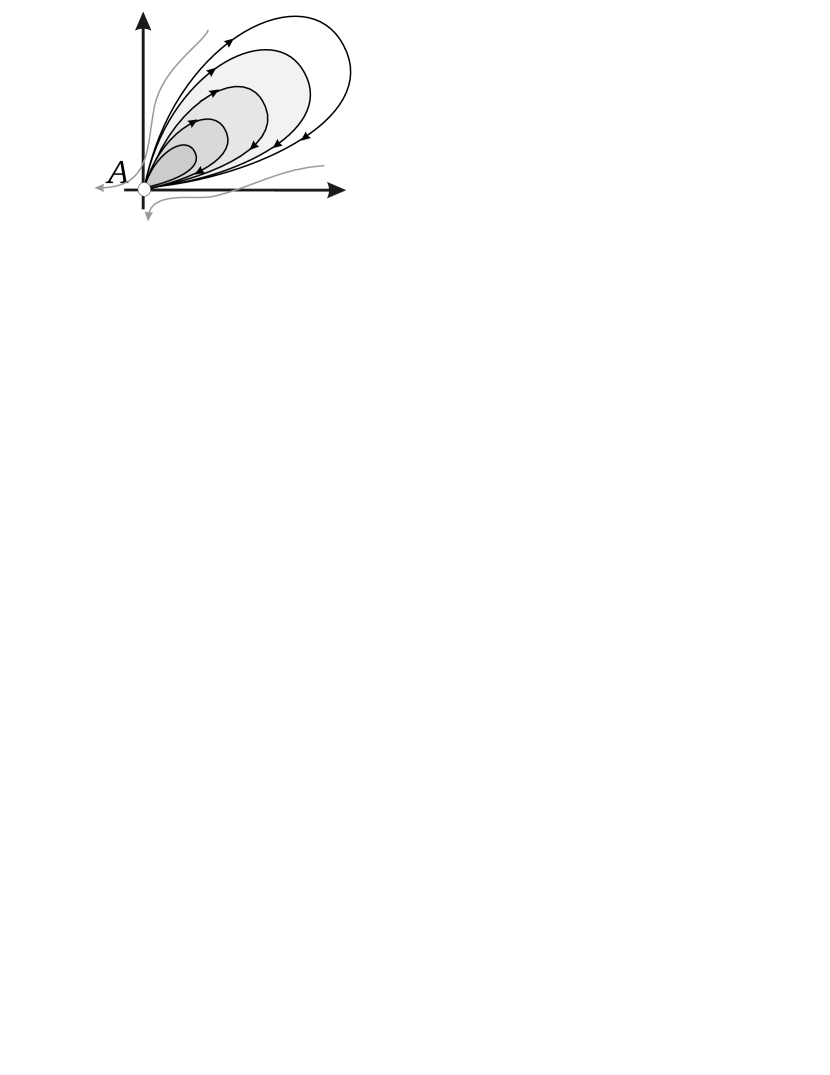
a

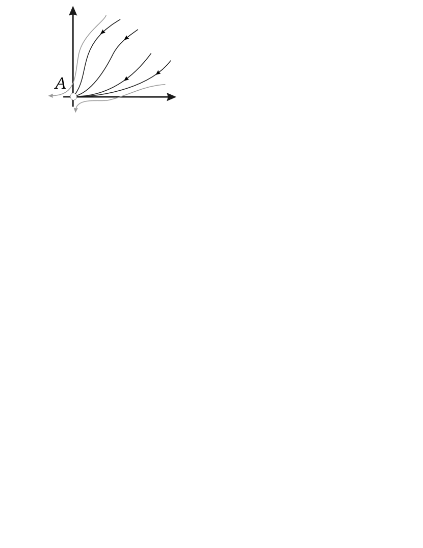
b

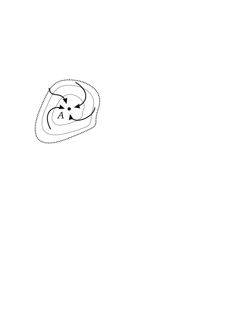
c

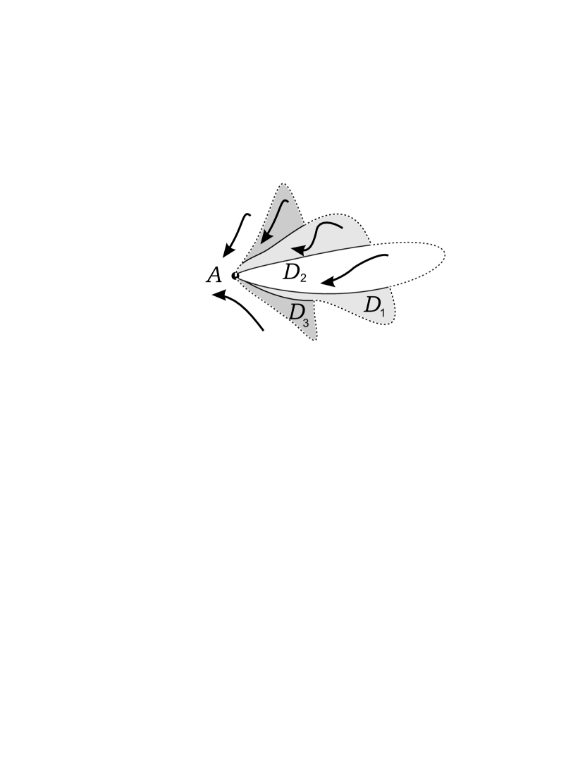
d

Figure 1: Panels a,b: a diagrammatic picture of an elliptic sector (panel a) and a parabolic sector (panel b) in the phase space of nonlinear systems [8]. Panel c: a system of neighborhoods corresponding to the level sets of a Lyapunov function of a stable set $A$. Every neighborhood is forward invariant; all trajectories are contained in the largest neighborhood (marked by dashed line). Panel d: a system of forward invariant sets of an attracting set $A$. Trajectories passing through the union of these sets (marked by dashed line) remain there in forward time.

illustrates (panels a,b), there are alternatives that do not comply with these assumptions. On the other hand techniques which can be used to address the questions above for equations (1), such as, e.g., [19], lack the convenience of the method of Lyapunov functions.

Recently, an approach has been proposed in [1] that enables to extend the method of Lyapunov functions to a class of systems with unstable invariant sets. Standard Lyapunov stability of a set is equivalent to existence of a nested family of neighborhoods, containing this set, which are forward-invariant with respect to dynamics of the system (Fig. 1, panel c). And the method of Lyapunov functions is a tool for finding such nested family of neighborhoods. In the approach proposed in [1] families of nested neighborhoods are replaced with collections of forward invariant sets containing the set of interest (Fig. 1, panel d). These sets are not necessarily neighborhoods of the invariant set. Yet, if they exist and at least one of such sets has a non-zero measure, then the original invariant set is clearly weakly attracting in Milnor’s sense [20].

Utility of proposed in [1] criteria specifying sets of forward-invariance, as well as their non-invariant counterparts, is that the resulting conditions are akin to the ones used in the method of Lyapunov functions and other tangential conditions [21], [22] (see also [23] for conditions of instability). This offers obvious advantage. On the other hand, few questions remain regarding the approach in [1], including a) existence of a similar analogue of Lyapunov’s first method, b) possibility of unstable yet exponential convergence and corresponding conditions, and c) how tight the derived conditions for boundedness and asymptotic convergence may be? Answering to these questions is the main goal of this work.

The paper is organized as follows. Main notational agreements and conventions are provided in Section II, Section III presents general class of systems considered in [1], main assumptions and one illustrative theoretical result. In Section IV we show how these results can be used to extend the first method of Lyapunov. Furthermore, for a subclass of systems relevant in problems of adaptive observers design, we provide conditions ensuring that not only that the concerned equilibrium is a weak attractor but also that the convergence to this attractor is exponential. Finally, we demonstrate that boundedness and attractivity conditions that the approach from [1] provides may sometimes be necessary too. Section V concludes the paper.

II Notation

The following notational conventions are used throughout the paper:

• $\mathbb{R}$ denotes the set of real numbers, $\mathbb{R}_{>a}=\{x\in\mathbb{R}\ |\ x>a\}$, and $\mathbb{R}_{\geq a}=\{x\in\mathbb{R}\ |\ x\geq a\}$;

• the Euclidean norm of $x\in\mathbb{R}^{n}$ is denoted by $\left\|x\right\|$, $\left\|x\right\|^{2}=x^{T}x$, where ^T stands for transposition;

• the space of $n\times n$ matrices with real entries is denoted by $\mathbb{R}^{n\times n}$; let $P\in\mathbb{R}^{n\times n}$, then $P>0$ ($P\geq 0$) indicates that $P$ is symmetric and positive (semi-)definite; $I_{n}$ denotes the $n\times n$ identity matrix;

• let $\Gamma\in\mathbb{R}^{n\times n}$, $\Gamma>0$, and $x\in\mathbb{R}$, then $\|x\|_{\Gamma^{-1}}^{2}$ denotes $x^{T}\Gamma^{-1}x$;

• by ${L}^{n}_{\infty}[t_{0},T]$, $t_{0}\in\mathbb{R}$, $T\in\mathbb{R},\ T\geq t_{0}$ we denote the space of all functions $xf:[t_{0},T]\rightarrow\mathbb{R}^{n}$ such that $\|f\|_{\infty,[t_{0},T]}={\mathrm{ess}}\sup\{\|f(t)\|,t\in[t_{0},T]\}<\infty$; $\|f\|_{\infty,[t_{0},T]}$ stands for the ${L}^{n}_{\infty}[t_{0},T]$ norm of $f(\cdot)$; if the function $f$ is defined on a set larger than $[t_{0},T]$ then notation $\|f\|_{\infty,[t_{0},T]}$ applies to the restriction of $f$ on $[t_{0},T]$;

• $\mathcal{C}^{r}$ denotes the space of continuous functions that are at least $r$ times differentiable;

• the symbol $\mathcal{K}_{0}$ denotes the set of all non-decreasing continuous functions $\kappa:\mathbb{R}_{\geq 0}\rightarrow\mathbb{R}_{\geq 0}$ such that $\kappa(0)=0$; $\mathcal{K}\subset\mathcal{K}_{0}$ is the subset of strictly increasing functions, and $\mathcal{K}_{\infty}\subset\mathcal{K}$ consists of functions from $\mathcal{K}$ with infinite limit: $\lim_{s\rightarrow\infty}\kappa(s)=\infty$.

III Preliminaries

Consider system (1)

$$\begin{split}\dot{x}&=f(x,\lambda,t),\\ \dot{\lambda}&=g(x,\lambda,t),\end{split}$$ (1)

where the vector-fields $f:\ \mathbb{R}^{n}\times\mathbb{R}\times\mathbb{R}\rightarrow\mathbb{R}^{n}$, $g:\ \mathbb{R}^{n}\times\mathbb{R}\times\mathbb{R}\rightarrow\mathbb{R}$ are continuous and locally Lipschitz w.r.t. $x$, $\lambda$ uniformly in $t$. The point $x=0,\lambda=0$ is assumed to be an equilibrium of (1).

Let $\mathcal{D}$ be an open subset of $\mathbb{R}^{n}$ and ${\Lambda}=[c_{1},c_{2}],\ c_{1}\leq 0,\ c_{2}>0$, be an interval. Suppose that the closure $\overline{\mathcal{D}}$ of $\mathcal{D}$ contains the origin, and denote $\mathcal{D}_{\Omega}=\overline{\mathcal{D}}\times{\Lambda}\times\mathbb{R}$. Finally, we suppose that the right-hand side of (1) satisfies Assumptions 1, 2 below.

Assumption 1

There exists a function $V:\mathbb{R}^{n}\rightarrow\mathbb{R}_{\geq 0}$, $V\in\mathcal{C}^{0}$, differentiable everywhere except possibly at the origin, and five functions of one variable, $\underline{\alpha},\bar{\alpha}\in\mathcal{K}_{\infty}$, $\alpha:\mathbb{R}_{\geq 0}\rightarrow\mathbb{R}$, $\alpha\in\mathcal{C}^{0}([0,\infty))$, $\alpha(0)=0$, $\beta:\ \mathbb{R}_{\geq 0}\rightarrow\mathbb{R}_{\geq 0}$, $\beta\in\mathcal{C}^{0}([0,\infty))$, $\varphi\in\mathcal{K}_{0}$ such that for every $(x,\lambda,t)\in{(\overline{\mathcal{D}}\setminus\{0\})\times\Lambda\times\mathbb{R}}$ the following properties hold:

$$\begin{split}\underline{\alpha}(\|x\|)\leq V(x)\leq\bar{\alpha}(\|x\|),\\ \frac{{\partial}V}{{\partial}x}f(x,\lambda,t)\leq\alpha(V(x))+\beta(V(x))\varphi(|\lambda|).\end{split}$$ (2)

Assumption 2

There exist functions $\delta,\xi\in\mathcal{K}_{0}$ such that the following inequality holds for all $(x,\lambda,t)\in{\mathcal{D}_{\Omega}}$:

$$\begin{split}-\xi(|\lambda|)-\delta(\|x\|)&\leq g(x,\lambda,t)\leq 0.\end{split}$$ (3)

The following is an example of a Lyapunov-like condition for establishing whether the origin of (1).

Corollary 1 ([1])

Consider system (1), and let $\mathcal{D}=\mathbb{R}^{n}$, $\Lambda=\mathbb{R}$. Suppose that Assumptions 1, 2 hold, there exists a function $\psi:\ \psi\in\mathcal{K}\cap\mathcal{C}^{1}((0,\infty))$ and a positive constant $a\in\mathbb{R}_{>0}$ such that for all $V\in(0,a]$

$$\begin{split}\frac{{\partial}\psi(V)}{{\partial}V}\left[\alpha(V)+\beta(V)\varphi(\psi(V))\right]\\ +\delta\left(\underline{\alpha}^{-1}(V)\right)+\xi\left(\psi(V)\right)\leq 0,\end{split}$$ (4)

Then

• the set

  $$\begin{split}\Omega_{a}=&\{(x,\lambda)\ |\ x\in\mathbb{R}^{n},\ \lambda\in\mathbb{R}_{\geq 0},\\ &\psi(a)\geq\lambda\geq\psi(V(x)),\ V(x)\in[0,a]\}\end{split}$$ (5)

  is forward invariant.

Furthermore, for every solution of (1) starting in $\Omega_{a}$

• there exists a limit

  $$\lim_{t\rightarrow\infty}\lambda(t)=\lambda^{\prime},\;\;\lambda^{\prime}\in[0,\psi(a)].$$

• If, in addition, the function $g(x,\lambda,\cdot)$ is uniformly continuous then:

  $$\lim_{t\rightarrow\infty}g(x(t),\lambda^{\prime},t)=0.$$

In the next section we show how this and other results from [1] can be used in extending classical Lyapunov’s first method. Furthermore, we will establish conditions ensuring exponential convergence of the solutions to the origin and show that sometimes these results may enable to derive necessary and sufficient conditions for existence of weak attractors in (1).

IV Main Results

IV-A Extension of Lyapunov’s First Method

Consider system

$$\begin{split}\dot{z}&=p(z)\end{split}$$ (6)

where the vector-field $p:\ \mathbb{R}^{m}\rightarrow\mathbb{R}^{m}$ is continuous and locally Lipschitz w.r.t. $z$. Furthermore, let it be differentiable at the origin, $p(0)=0$, and

$$J=\frac{{\partial}p}{{\partial}z}(0)$$

be the corresponding Jacobian matrix. Finally, let

$$\sigma_{1},\sigma_{2},\dots,\sigma_{m}$$

be the eigenvalues of $J$ with $\sigma_{1}=0$ and real parts of all other eigenvalues be negative. In what follows we are interested in finding a set of simple Lyapunov-like conditions that would enable us to establish whether the origin is a weak attractor or not.

Without loss of generality, consider dynamics of (6) in the coordinates

$$\left(\begin{array}[]{c}x\\ \lambda\end{array}\right)=Tz,$$

$x\in\mathbb{R}^{n}$, $\lambda\in\mathbb{R}$, $m=n+1$, where the $m\times m$ non-singular matrix $T$ is such that the structure of $TJT^{-1}$ is as follows

$$TJT^{-1}=\left(\begin{array}[]{cc}A&b\\ 0&0\end{array}\right),\ A\in\mathbb{R}^{n\times n},\ b\in\mathbb{R}^{n}.$$

It is clear that such matrix $T$ will always exist and that $\sigma_{2},\dots,\sigma_{m}$ are the eigenvalues of $A$.

Dynamics of (6) in the coordinates $(x,\lambda)$ is

$$\begin{split}\dot{x}&=f(x,\lambda)\\ \dot{\lambda}&=g(x,\lambda),\end{split}$$ (7)

with

$$\begin{split}\frac{{\partial}f}{{\partial}x}(0,0)=A,\ \frac{{\partial}f}{{\partial}\lambda}(0,0)=b,\\ \frac{{\partial}g}{{\partial}x}(0,0)=0,\ \frac{{\partial}g}{{\partial}\lambda}(0,0)=0.\end{split}$$

The following can now be formulated for (7)

Theorem 1

Consider system (7), and let the function $g$ be differentiable at least twice. Let $G$ be the Hessian of $g$ at the origin and let $G$ be sign-definite.

Then $(0,0)$ is a weak (Milnor) attractor for (7).

Proof:

Consider dynamics of (7) in a vicinity of the origin:

$$\begin{split}\dot{x}&=Ax+b\lambda+o(\|(x,\lambda)\|)\\ \dot{\lambda}&=\frac{1}{2}(x,\lambda)^{T}G(x,\lambda)(x,\lambda)+o(\|(x,\lambda)\|^{2}).\end{split}$$

Since real parts of the eigenvalues of $A$ are negative, there are symmetric positive-definite matrices $H$, $Q$ such that

$$HA+A^{T}H\leq-Q.$$

Without loss of generality suppose that $G<0$ (if $G>0$ we can replace $\lambda$ with $\tilde{\lambda}=-\lambda$ to get a system representation as in (7) but with $G<0$).

Let $V=x^{T}Hx$ and consider the function $\psi(V)=k\sqrt{V}$, $k>0$. It is clear that there exist $\alpha>0$, $\beta>0$, and $c_{1}>0$, independent on $k$, such that

$$\dot{V}\leq-\alpha V+\beta\sqrt{V}|\lambda|+c_{1}\sqrt{V}|o(\|(x,\lambda)\|)|.$$

Furthermore, for any given $\varepsilon>0$ there is a neighborhood $\Omega_{1}$ of the origin:

$$|o(\|(x,\lambda)\|)|\leq\varepsilon(\sqrt{V(x)}+|\lambda|)\ \mathrm{for\ all}\ (x,\lambda)\in\Omega_{1}.$$

Hence there exists a neighborhood $\Omega_{2}$ of the origin and $\alpha_{1}>0$, $\beta_{1}>0$, independent on $k$:

$$\dot{V}\leq-\alpha_{1}V(x)+\beta_{1}\sqrt{V(x)}|\lambda|\ \mathrm{for\ all}\ (x,\lambda)\in\Omega_{2}.$$

Similarly, there is a neighborhood $\Omega_{3}$ containing the origin and a constant $\gamma>0$ such that

$$-\gamma(V(x)+\lambda^{2})\leq\dot{\lambda}\leq 0\ \mathrm{for\ all}\ (x,\lambda)\in\Omega_{3}.$$

According to [1] (Lemma 1) existence of an interval $(0,a]$, $a>0$ such that

$$\begin{split}\frac{{\partial}\psi}{{\partial}V}(-\alpha_{1}V+\beta_{1}\sqrt{V}\psi(V))+\gamma V+\gamma\psi^{2}(V)\leq 0\end{split}$$ (8)

would imply that the intersection of the corresponding sets $\Omega_{a}$ and $\Omega_{2}\cap\Omega_{3}$ is forward-invariant. Substituting $\psi(V)=k\sqrt{V}$ into the left-hand side of the expression above one obtains

$$\begin{split}&-k\frac{\alpha_{1}}{2}\sqrt{V}+k^{2}\frac{\beta_{1}\sqrt{V}}{2}+\gamma(V+k^{2}V)=\\ &\sqrt{V}(-k\frac{\alpha_{1}}{2}+k^{2}\frac{\beta_{1}}{2}+\gamma(1+k^{2})\sqrt{V}).\end{split}$$

It is therefore clear that (8) holds for all

$${V}\leq a=\left[\left(k\frac{\alpha_{1}}{2}-k^{2}\frac{\beta_{1}}{2}\right)/(\gamma(1+k^{2}))\right]^{2}.$$

The measure of the set $\Omega_{a}$ ($a\neq 0$) is non-zero. Moreover, since $G$ is sign-definite,

$$\lim_{t\rightarrow\infty}x(t)=0,\ \lim_{t\rightarrow\infty}\lambda(t)=0.$$

Hence $(0,0)$ is a weak attractor. ∎

IV-B Exponential Convergence

Consider a subclass of (1) that is relevant in the problem of adaptive observer design [15]:

$$\begin{split}\left(\begin{array}[]{c}\dot{x}_{1}\\ \dot{x}_{2}\end{array}\right)&=\left(\begin{array}[]{cc}A&b\varphi^{T}(t)\\ -\Gamma\varphi(t)C^{T}&0\end{array}\right)\left(\begin{array}[]{c}{x}_{1}\\ {x}_{2}\end{array}\right)\\ &+\left(\begin{array}[]{c}b\\ 0\end{array}\right)v(t,\lambda)\\ \dot{\lambda}&=-\gamma|C^{T}x_{1}|,\\ &x=(x_{1},x_{2}),\ x(t_{0})=x_{0},\ \lambda(t_{0})=\lambda_{0},\end{split}$$ (9)

where $x_{1}\in\mathbb{R}^{k}$, $x_{2}\in\mathbb{R}^{m}$, $\lambda\in\mathbb{R}$ are state variables ($k+m=n$), $x_{0}\in\mathbb{R}^{n}$, $\lambda_{0}>0$ are initial conditions, $\Gamma\in\mathbb{R}^{m\times m}$ is a positive-definite symmetric matrix; matrix $A\in\mathbb{R}^{k\times k}$, and vectors $b$, $C$ are supposed to satisfy

$$\left\{\begin{split}&PA+A^{T}P\leq-Q\\ &Pb=C.\end{split}\right.$$ (10)

for some symmetric positive definite matrices $P$, $Q$. Functions $\varphi:\mathbb{R}\rightarrow\mathbb{R}^{m}$, $v:\mathbb{R}\times\mathbb{R}\rightarrow\mathbb{R}$ are continuous and differentiable with bounded derivatives. Furthermore, $v(t,0)=0$ for all $t$.

It has been shown in [15] that if the function $\varphi$ is persistently exciting, bounded and with bounded derivative then there exists an interval $(0,\gamma^{\ast}(x_{0},\lambda_{0})]$, $\gamma^{\ast}(x_{0},\lambda_{0})>0$, such that for all constant $\gamma$ taken from this interval solutions of (9) are bounded and $0<\lambda(t)<\lambda_{0}\ \forall\ t\geq t_{0}$. Furthermore, $\lim_{t\rightarrow\infty}\lambda(t)=0$ and $\lim_{t\rightarrow\infty}x(t)=0$. One can arrive at the same conclusion using e.g. Corollary 1 or Lemma 1 from [1]. The question, however, is if such convergence can be made exponential. An answer to this question is provided below.

Theorem 2

Consider system (9) with $A,b,C$ satisfying (10). Let us suppose that parameter $\gamma$ and initial conditions are chosen so that solutions of (9) are bounded. Furthermore, let the vector

$$\phi(t)=\left(\varphi(t),\left.\int_{0}^{1}\frac{{\partial}v(t,a)}{{\partial}a}\right|_{a=\lambda(t)s}ds\right)$$

be persistently exciting

$$\exists\ T,\mu>0:\ \int_{t}^{t+T}\phi(\tau)\phi(\tau)^{T}d\tau\geq\mu I_{m+1}\ \forall t\geq t_{0},$$

and there is an $M_{\phi}>0$: $\max\{\|{\phi}(t)\|,\|\dot{\phi}(t)\|\}<M_{\phi}$ for all $t\geq t_{0}$. Then $x(t)$, $\lambda(t)$ converge to the origin exponentially fast.

Proof:

The proof is organized as follows. First, we demonstrate that for all $t,t_{0}$, $t\geq t_{0}$ (for which the solutions are defined) the vectors $x_{1}(t)$ and $q(t)=(x_{2}(t),\lambda(t))$ satisfy the following conditions:

• $\exists\ c_{1}:\ \|x_{1}\|_{\infty,[t,\infty)}\leq c_{1}(\|x_{1}(t)\|+\|q(t)\|)\ \forall\ t\geq t_{0}$

• $\exists\ c_{2}:\ \|q\|_{\infty,[t,\infty)}\leq c_{2}(\|x_{1}(t)\|+\|q(t)\|)\ \forall\ t\geq t_{0}$

• $\exists\ c_{3}:\ \|x_{1}\|_{2,[t,\infty)}\leq c_{3}(\|x_{1}(t)\|+\|q(t)\|)\ \forall\ t\geq t_{0}$,

where $c_{1}$,$c_{2}$, and $c_{3}$ are independent of $t$. Second, we show that

• $\exists\ c_{4}:\ \|q\|_{2,[t,\infty)}\leq c_{4}(\|x_{1}(t)\|+\|q(t)\|)$.

Finally, we invoke a result from [24],[25] to show that C1–C4 imply exponential convergence of the observer.

Lemma 1

Let $x:\mathbb{R}\rightarrow\mathbb{R}^{n}$ be a function satisfying

$$\max\{\|x\|_{2,[t,\infty)},\|x\|_{\infty,[t,\infty)}\}\leq c\|x(t)\|,\ \forall\ t\geq t_{0}.$$ (11)

Then

$$\|x(t)\|\leq ce^{1/2}e^{-\frac{t-t_{1}}{2c^{2}}}\|x(t_{1})\|,\ \forall\ t\geq t_{1}\geq t_{0}.$$

First part. We have that for all $t\geq t_{1}\geq t_{0}$

$$0\leq\lambda(t)\leq\lambda(t_{1})-\gamma\int_{t_{1}}^{t}|C^{T}x_{1}(\tau,x_{0})|d\tau.$$

Let $P>0$ be a matrix satisfying (10). Consider the following function

$$V=x_{1}^{T}Px_{1}+\|x_{2}\|^{2}_{\Gamma^{-1}}+\frac{D_{v}}{\gamma}\lambda^{2},$$

where $D_{v}$ is $\max_{t\geq t_{0},\ \lambda\in[0,\lambda_{0}]}|{\partial}v(t,\lambda)/{\partial}\lambda|$. It is clear that

$$\begin{split}\dot{V}&\leq-x_{1}^{T}Qx_{1}+2x_{1}^{T}Pb\varphi^{T}(t)x_{2}-2x_{2}^{T}C^{T}x_{1}\varphi(t)\\ &+2x_{1}^{T}Pbv(t,\lambda)-2D_{v}\lambda|C^{T}x_{1}|\leq-x_{1}^{T}Qx_{1}\\ &-2|C^{T}x_{1}|(D_{v}\lambda-\mathrm{sign}(C^{T}x_{1})v(t,\lambda)).\end{split}$$ (12)

Noticing that $\lambda(t)\geq 0$,

$$v(t,\lambda)=v(t,\lambda)-v(t,0)=\int_{0}^{1}\left.\frac{{\partial}v(t,a)}{{\partial}a}\right|_{a=s\lambda}ds\lambda,$$

and consequently,

$$|\mathrm{sign}(C^{T}x_{1})v(t,\lambda)|\leq D_{v}\lambda,$$

we can conclude that the term $D_{v}\lambda-\mathrm{sign}(C^{T}x_{1})v(t,\lambda)$ in (12) is always non-negative, and hence

$$\dot{V}\leq-x_{1}^{T}Qx_{1}.$$ (13)

Thus C1, C2 hold. Furthermore, in view of (13), one can derive that C3 holds as well.

Second part. Let us show that C4 holds. In order to do so we use the method described in [25]. Consider the variable

$$z=q-\phi(t)b^{T}x_{1}$$

and calculate its derivative:

$$\dot{z}=\dot{q}-\dot{\phi}(t)b^{T}x_{1}-{\phi}(t)b^{T}Ax_{1}-{\phi}(t)b^{T}b(\varphi(t)^{T}x_{2}+v(t,\lambda)).$$

Noticing that $v(t,\lambda)=\int_{0}^{1}\left.\frac{{\partial}v(t,a)}{{\partial}a}\right|_{a=s\lambda}ds\lambda$ we conclude that

$$\varphi(t)^{T}x_{2}+v(t,\lambda)=\phi(t)^{T}(x_{2},\lambda)=\phi(t)^{T}q.$$

Hence

$$\begin{split}\dot{z}=&\dot{q}-\dot{\phi}(t)b^{T}x_{1}-{\phi}(t)b^{T}Ax_{1}-{\phi}(t)b^{T}b\phi(t)^{T}z\\ &-\phi(t)b^{T}b\phi(t)^{T}\phi(t)^{T}bx_{1}\\ =&-\phi(t)b^{T}b\phi(t)^{T}z+\chi(t,x_{1}),\end{split}$$

where

$$\begin{split}\chi(t,x_{1})=&\dot{q}-\dot{\phi}(t)b^{T}x_{1}-\\ &\phi(t)b^{T}Ax_{1}-\phi(t)b^{T}b\phi(t)^{T}\phi(t)^{T}bx_{1}.\end{split}$$

Recall that $\dot{q}=\mathrm{col}(-\Gamma\varphi(t)C^{T}x_{1},-\gamma|C^{T}x_{1}|)$ and that $\phi(t),\dot{\phi}(t)$ are bounded. Hence there is a constant $M>0$ such that

$$\|\chi(t,x_{1})\|\leq M\|x_{1}\|.$$

Taking into account that $\phi(t)$ is persistently exciting we can conclude that there are constants $\beta_{1},\beta_{2}$:

$$\|z\|_{2,[t,\infty)}\leq\beta_{1}\|z(t)\|+\beta_{2}\|x_{1}\|_{2,[t,\infty)}.$$

for all $t\geq t_{0}$. Given that $\|\phi(t)b^{T}x_{1}\|\leq M_{\phi}\|b\|\|x_{1}\|$ we obtain:

$$\begin{split}\|q\|_{2,[t,\infty)}\leq&\beta_{1}(\|q(t)\|+M_{\phi}\|b\|\|x_{1}(t)\|)\\ &+(M_{\phi}\|b\|+\beta_{2})\|x_{1}\|_{2,[t,\infty)}.\end{split}$$

Hence C4 holds.

Third part follows from Lemma 1. ∎

IV-C How tight are the estimates of regions of forward invariance?

On the one hand, since Assumptions 1 and 2 are inherently conservative, our results bear a degree of conservatism. On the other hand, if viewed as conditions for the mere existence of (weakly) attracting sets, they can sometimes be remarkably precise. This is illustrated with the example below.

Example 1

Consider system

$$\begin{split}\dot{x}_{1}&=-\tau_{1}x_{1}+c_{1}x_{2}\\ \dot{x}_{2}&=-c_{2}|x_{1}|,\ \tau_{1},\ c_{1},\ c_{2}\in\mathbb{R}_{>0},\end{split}$$ (14)

and let us determine the values of $c_{1},c_{2}$, and $\tau_{1}$ such that the origin is a weak attractor for (14). We will do this by invoking Corollary 1. It is clear that solutions of (14) are defined for all $t$. Thus letting $\mathcal{D}_{x}=\mathbb{R}$, $\mathcal{D}_{\lambda}=\mathbb{R}$ we can easily see that Assumption 1 holds for the first equation with $V(x_{1})=x_{1}^{2}$:

$$\dot{V}\leq-2\tau_{1}V+2c_{1}\sqrt{V}|x_{2}|,$$

and Assumption 2 is satisfied for the second equation with $\delta(|x_{1}|)=c_{2}|x_{1}|=c_{2}\sqrt{V}$, $\xi(|x_{2}|)=0$. Let us pick

$$\psi(V)=p\sqrt{V},\ p\in\mathbb{R}_{>0},$$

and consider

$$\begin{split}&\frac{{\partial}\psi}{{\partial}V}(-2\tau_{1}V+2c_{1}\sqrt{V}\psi(V))\\ &\ \ \ \ +c_{2}\sqrt{V}=(-p\tau_{1}+c_{1}p^{2}+c_{2})\sqrt{V}.\end{split}$$ (15)

The expression above is defined for $V\in(0,\infty)$, and it is non-positive for $c_{2}\leq p(\tau_{1}-pc_{1})$. The right-hand side of the last inequality is maximal at $p=\tau_{1}/(2c_{1})$. Thus we can conclude that

$$c_{2}\leq\frac{\tau_{1}^{2}}{4c_{1}}$$ (16)

ensures that (15) is non-positive for all $V\in\mathbb{R}_{>0}$. Hence, according to Corollary 1, the set

$$\Omega=\{(x_{1},x_{2})\ |x\in\mathbb{R},\ x_{2}\in\mathbb{R}_{>0},\ x_{2}\geq\frac{\tau_{1}}{2c_{1}}|x_{1}|\}$$

is forward-invariant. Moreover, solutions of (14) starting in $\Omega$ are bounded and satisfy $\lim_{t\rightarrow\infty}x_{1}(t)=0$. Given that $x_{2}(t)$ is bounded, Barbalatt’s lemma (applied to the first equation) implies that $\lim_{t\rightarrow\infty}x_{2}(t)=0$. Hence, the origin of system (14) satisfying condition (16) is a weak attractor.

Let us now see if the attractor persists when inequality (16) does not hold. Consider an auxiliary system:

$$\begin{split}\dot{x}_{1}&=-\tau_{1}x_{1}+c_{1}x_{2}\\ \dot{x}_{2}&=-c_{2}x_{1},\ \tau_{1},\ c_{1},\ c_{2}\in\mathbb{R}_{>0},\end{split}$$ (17)

and let $(x_{1}(t),x_{2}(t))$ be a non-trivial solution of (17). If the roots of $\chi(s)=s^{2}+\tau_{1}s+c_{1}c_{2}$ have non-zero imaginary real parts then the sign of $x_{2}(t)$ will necessarily alternate. This, however, implies that no non-trivial solutions of (14) converge to the origin. The roots of $\chi(s)$ are real, however, only if (16) holds. Therefore, in this particular case, condition (16) is not only sufficient but it is also necessary for the origin of (14) to be an attractor.

Phase curves of (14) illustrating this point are provided in Fig. 2. The left plot corresponds to the case when condition (16) is satisfied. As we can see, solutions are asymptotically approaching the origin (marked by a black circle). The right plot shows phase curves of the system in which the value of $c_{2}$ is larger than $\tau_{1}^{2}/(4c_{1})$. In this case, as can be clearly seen in the inset at the bottom right corner, solutions of the system do not approach the origin asymptotically. They are lingering in its neighborhood for a while, and then eventually escape.

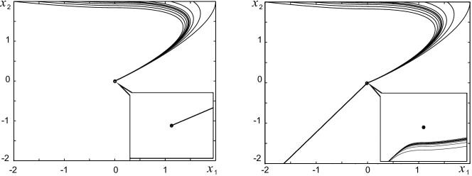
Figure 2: Plots of the phase curves of system (14) passing through the line $x_{2}(0)=2$. Parameters $\tau_{1}=1,c_{1}=1$ were fixed in all simulations, and parameter $c_{2}$ was varying. Left panel: phase curves of (14) for $c_{2}=1/4$. Right panel: phase curves of the system for $c_{2}=11/40$. Insets in the bottom right corner of each plot show behavior of the phase curves within the rectangle $[-2\cdot 10^{-4},2\cdot 10^{-4}]\times[-2\cdot 10^{-4},2\cdot 10^{-4}]$, that is in the close proximity to the origin.

Finally, we would also like to remark that conditions presented in e.g. Corollary 1 can, in principle, be less conservative than the ones established previously in the framework of input-output/state analysis, cf. [19]. Indeed, when applied to the same system, (14), Corollary 4.1 from [19] yields the following upper bound for $c_{2}$:

$$c_{2}<\frac{1}{16}\frac{\tau_{1}^{2}}{c_{1}},$$

which is four times smaller than the one derived from Corollary 1.

V Conclusion

In this manuscript we presented several results that are immediate consequences of our earlier published work [1]. These results enabled to extend first method of Lyapunov for the analysis of asymptotic behavior of solutions in a vicinity of an equilibrium to systems in which the corresponding Jacobian has one zero eigenvalue. We showed that the fact that all other eigenvalues have negative real parts coupled with sign-definiteness condition of an associated quadratic form is sufficient to warrant that the equilibrium is a weak (Milnor) attractor. In particular, for $\dot{z}=p(z)$ with $p:\mathbb{R}^{m}\rightarrow\mathbb{R}^{m}$ differentiable at least twice, let

• $J$ be the Jacobian of the vector-filed $p$ at the origin,

• $\sigma_{1}\dots,\sigma_{m}$ be the eigenvalues of $J$ with $\sigma_{1}=0$ and $Re(\sigma_{k})<0$, $k=2,\dots,m$,

• $T$ be a similarity transform such that the last row of $TJT^{-1}$ is zero

• $g(x)$ be the $m$-th component of $Tp(T^{-1}x)$, and

• $G$ be the Hessian matrix of $g$.

Then the origin is a (local) weak attractor if $G$ is sign-definite.

Furthermore we provided analysis of convergence rates for a relevant subclass of systems with unstable attractors. We have shown that persistency of excitation plays an important role in establishing exponential convergence to the attractor. Finally, we demonstrated that conditions presented in the original work [1] can be remarkably tight, at least for some example problems. Several questions, however, still remain. One of these is how (and if) the established rate of convergence may change in presence of unmodeled dynamics providing that the modulus is replaced with a dead-zone in (9). Answering to these is the subject of ongoing work.

References

• [1] A. Gorban, I. Tyukin, E. Steur, and H. Nijmeijer, “Lyapunov-like conditions of forward invariance and boundedness for a class of unstable systems,” SIAM Journal on Control and Optimization, vol. 51, no. 3, pp. 2306 –2334, 2013.
• [2] A. Lyapunov, The general problem of the stability of motion (in Russian).   Kharkov Mathematical Society, 1892, republished by the University of Toulouse, 1908 and Princeton University Press, 1949 (in French). Republished in English by Int. Journal of Control, 1992.
• [3] H. Nijmeijer and A. van der Schaft, Nonlinear Dynamical Control Systems.   Springer–Verlag, 1990.
• [4] A. Isidori, Nonlinear control systems: An Introduction, 2nd ed.   Springer–Verlag, 1989.
• [5] L. Ljung, System Identification: Theory for the User.   Prentice Hall, 1999.
• [6] K. S. Narendra and A. M. Annaswamy, Stable Adaptive systems.   Prentice–Hall, 1989.
• [7] A. Andronov, E. Leontovich, I. Gordon, and M. A.G., Qualitative Theory of Second-order Dynamic Systems.   Halsted Press, New York, 1973.
• [8] N. Bautin and E. Leontovich, Methods and means for a qualitative investigation of dynamical systems on the plane.   Nauka, Moscow, 1990.
• [9] M. I. Rabinovic, P. Varona, A. Selverston, and H. Abarbanel, “Dynamical principles in neuronscience,” Reviews of Modern Physics, vol. 78, pp. 1213–1265, 2006.
• [10] M. I. Rabinovic, R. Huerta, P. Varona, and V. Aframovich, “Transient cognitive dynamics, metastability, and decision-making,” PLOS Computational Biology, vol. 4, no. 5, pp. 1–9, 2008.
• [11] I. Tyukin, T. Tyukina, and C. van Leeuwen, “Invariant template matching in systems with spatiotemporal coding: a vote for instability,” Neural Networks, vol. 22, no. 4, pp. 425–449, 2009.
• [12] M. Goman and M. Demenkov, “Multiple attractor dynamics in active flutter suppression problem,” in ICNPAA 2008: Mathematical Problems in Engineering, Genoa, Italy, June 2008.
• [13] A. Ilchmann, “Universal adaptive stabilization of nonlinear systems,” Dynamics and Control, no. 7, pp. 199–213, 1997.
• [14] J.-B. Pomet, “Remarks on sufficient information for adaptive nonlinear regulation,” in Proceedings of the 31-st IEEE Control and Decision Conference, 1992, pp. 1737–1739.
• [15] I. Tyukin, E. Steur, H. Nijmeijer, and C. van Leeuwen, “Adaptive observers and parameter estimation for a class of systems nonlinear in parameters,” Automatica, vol. 49, no. 8, pp. 2409–2423, 2013.
• [16] A. Rantzer, “A dual to Lyapunov’s stability theorem,” Systems and Control Letters, vol. 42, no. 3, pp. 161–168, 2001.
• [17] I. Masubuchi, “Analysis of positive invariance and almost regional attraction via density functions with converse results,” IEEE Trans. Automat. Contr., vol. 52, no. 7, pp. 1329–1333, 2007.
• [18] I. Vadia and M. P.G., “Lyapunov measure for almost everywhere stability,” IEEE Trans. Automat. Contr., vol. 53, no. 1, pp. 307–323, 2008.
• [19] I. Tyukin, E. Steur, H. Nijmeijer, and C. van Leeuwen, “Non-uniform small-gain theorems for systems with unstable invariant sets,” SIAM Journal on Control and Optimization, vol. 47, no. 2, pp. 849–882, 2008.
• [20] J. Milnor, “On the concept of attractor,” Commun. Math. Phys., vol. 99, pp. 177–195, 1985.
• [21] J.-P. Aubin, “Viability solutions to structured Hamilton-Jacobi equations under constraints,” SIAM J. Control Optim., vol. 49, no. 5, pp. 1881–1915, 2011.
• [22] M. Nagumo, “$\ddot{\mathrm{U}}$ber die lage der integralkurven gew$\ddot{\mathrm{o}}$hnlicher differentialgleichungen,” Proc. Phys. Math. Soc. Japan, vol. 24, pp. 551–559, 1942.
• [23] N. Chetaev, The stability of motion.   Pergamon Press, 1961.
• [24] I. Tyukin, Adaptation in Dynamical Systems.   Cambridge Univ. Press, 2011.
• [25] A. Loria and E. Panteley, “Uniform exponential stability of linear time-varying systems: revisited,” Systems and Control Letters, vol. 47, no. 1, pp. 13–24, 2002.