Multiple chessboard complexes
and the colored Tverberg problem

Abstract

Following D.B. Karaguezian, V. Reiner, and M.L. Wachs (Matching Complexes, Bounded Degree Graph Complexes, and Weight Spaces of $GL$-Complexes, Journal of Algebra 2001) we study the connectivity degree and shellability of multiple chessboard complexes. Our central new results (Theorems 3.2 and 4.4) provide sharp connectivity bounds relevant to applications in Tverberg type problems where multiple points of the same color are permitted. These results also provide a foundational work for the new results of Tverberg-van Kampen-Flores type, as announced in the forthcoming paper [JVZ-2].

1 An overview and motivation

Chessboard complexes and their generalizations belong to the class of most studied graph complexes, with numerous applications in and outside combinatorics [A04, BLVŽ, BMZ, FH98, G79, J08, KRW, M03, SW07, VŽ94, ŽV92, Zi11, Ž04].

The connectivity degree of a simplicial complex was selected in [J08, Chapter 10] as one of the five most important and useful parameters in the study of simplicial complexes of graphs. Following [KRW] we study the connectivity degree of multiple chessboard complexes (Section 1.4) and their generalizations (Section 2). Our first central result is Theorem 3.2 which improves the $2$-dimensional case of [KRW, Corollary 5.2.] and reduces to the $2$-dimensional case of [BLVŽ, Theorem 3.1.] in the case of standard chessboard complexes.

Perhaps it is worth emphasizing that our methods allow us to obtain sharp bounds relevant to applications in Tverberg and van Kampen-Flores type problems (see Section 5.1 and [JVZ-2]). Moreover, the focus in [KRW] is on the homology with the coefficients in a field and multidimensional chessboard complexes while our results are homotopical and apply to $2$-dimensional chessboard complexes.

High connectivity degree is sometimes a consequence of the shellability of the complex (or one of its skeletons), see [Zi94] for an early example in the context of chessboard complexes. Theorem 4.4 provides a sufficient condition which guarantees the shellability of multiple chessboard complexes and yields another proof of Theorem 3.2. The construction of the shelling offers a novel point of view on this problem and seems to be new and interesting already in the case of standard chessboard complexes.

Among the initial applications of the new connectivity bounds established by Theorem 3.2 is a result of colored Tverberg type where multiple points of the same color are permitted (Theorem 5.1 in Section 5). After the first version of our paper was submitted to the arXiv we were kindly informed by Günter Ziegler that Theorem 5.1 is implicit in their recent work (see [BFZ], Theorem 4.4 and the remark following the proof of Lemma 4.2.).

Other, possibly more far reaching applications of Theorems 3.2 and 4.4 to theorems of Tverberg-van Kampen-Flores type are announced in [JVZ-2]. This provides new evidence that the chessboard complexes and their generalizations are a natural framework for constructing configuration spaces relevant to Tverberg type problems and related problems about finite sets of points in Euclidean spaces.

Caveat: Most if not all simplicial complexes in this paper are visualized in a rectangular chessboard $[m]\times[n]$. The reader is free to choose either the Cartesian or the matrix enumeration of squares (where $(1,1)$ is the lower left corner in the first and the upper left corner in the second). This should not generally affect the reading of the paper and a little care is needed only when interpreting the Figure 1, revealing our slight inclination towards the Cartesian notation.

1.1 Colored Tverberg problems

‘Tverberg problems’ is a common name for a class of theorems and conjectures about finite sets of points (point clouds) in $\mathbb{R}^{d}$. We start with a brief introduction into this area of topological combinatorics emphasizing, in the spirit of [Ž99] and [VŽ11], a graphical or diagrammatic ((2)-(6)) presentation of these results. The reader is referred to [Zi11], [VŽ11, Section 14.4], [Ž04], and [M03] for more complete expositions of these problems and the history of the whole area.

The Tverberg theorem [T66] claims that every set $K\subset\mathbb{R}^{d}$ with $(d+1)(q-1)+1$ elements can be partitioned $K=K_{1}\cup\ldots\cup K_{q}$ into $q$ nonempty, pairwise disjoint subsets $K_{1},\ldots,K_{q}$ such that the corresponding convex hulls have a nonempty intersection:

$$\bigcap_{i=1}^{q}{\rm conv}(K_{i})\neq\emptyset.$$ (1)

Following [BSS] it can be reformulated as the statement that for each linear (affine) map $f:\Delta^{D}\stackrel{{\scriptstyle a}}{{\longrightarrow}}\mathbb{R}^{d}$ ($D=(d+1)(q-1)$) there exist $q$ nonempty disjoint faces $\Delta_{1},\ldots,\Delta_{q}$ such that $f(\Delta_{1})\cap\ldots\cap f(\Delta_{q})\neq\emptyset$. This form of Tverberg’s result can be summarized as follows,

$$(\Delta^{(d+1)(q-1)}\stackrel{{\scriptstyle a}}{{{\longrightarrow}}}\mathbb{R}^{d})\Rightarrow(q-{\rm intersection}).$$ (2)

Here we tacitly assume that the faces intersecting in the image are always vertex disjoint. The letter “a” over the arrow means that the map is affine and its absence indicates that it can be an arbitrary continuous map.

The following four statements are illustrative for results of ‘colored Tverberg type’.

$$(K_{3,3}\longrightarrow{\mathbb{R}}^{2})\Rightarrow(2-{\rm intersection})$$ (3)

$$(K_{3,3,3}\stackrel{{\scriptstyle a}}{{{\longrightarrow}}}{\mathbb{R}}^{2})\Rightarrow(3-{\rm intersection})$$ (4)

$$(K_{5,5,5}\longrightarrow{\mathbb{R}}^{3})\Rightarrow(3-{\rm intersection})$$ (5)

$$(K_{4,4,4,4}\longrightarrow{\mathbb{R}}^{3})\Rightarrow(4-{\rm intersection})$$ (6)

$K_{t_{1},t_{2},\ldots,t_{k}}=[t_{1}]\ast[t_{2}]\ast\ldots\ast[t_{k}]$ is by definition the complete multipartite simplicial complex obtained as a join of $0$-dimensional complexes (finite sets). By definition the vertices of this complex are naturally partitioned into groups of the same ‘color’. For example $K_{p,q}=[p]\ast[q]$ is the complete bipartite graph obtained by connecting each of $p$ ‘red vertices’ with each of $q$ ‘blue vertices’. The simplices of $K_{t_{1},t_{2},\ldots,t_{k}}$ are called multicolored sets or rainbow simplices and its dimension is $k_{-}=k-1$. (We systematically use the abbreviation $a_{-}:=a-1$ to emphasize that $a_{-}$ is the dimension of a non-degenerate simplex with $a$ vertices.)

The implication (3) says that for each continuous map $\phi:K_{3,3}\rightarrow\mathbb{R}^{2}$ there always exist two vertex-disjoint edges which intersect in the image. In light of the Hanani-Tutte theorem this statement is equivalent to the non-planarity of the complete bipartite graph $K_{3,3}$. The implication (4) is an instance of a result of Bárány and Larman [BL]. It says that each collection of nine points in the plane, evenly colored by three colors, can be partitioned into three multicolored or ‘rainbow triangles’ which have a common point.

Note that a $9$-element set $C\subset\mathbb{R}^{2}$ which is evenly colored by three colors, can be also described by a map $\alpha:[3]\sqcup[3]\sqcup[3]\rightarrow\mathbb{R}^{2}$ from a disjoint sum of three copies of $[3]$. In the same spirit an affine map $\phi:K_{3,3,3}\stackrel{{\scriptstyle a}}{{\longrightarrow}}\mathbb{R}^{2}$ parameterizes not only the colored set itself but takes into account from the beginning that some simplices (multicolored or rainbow simplices) play a special role.

A similar conclusion has statement (5) which is a formal analogue of the statement (3) in dimension $3$. It is an instance of a result of Vrećica and Živaljević [VŽ94], which claims the existence of three intersecting, vertex disjoint rainbow triangles in each constellation of $5$ red, $5$ blue, and $5$ green stars in the $3$-space. A consequence of this result is that $K_{5,5,5}$ is strongly non-embeddable in $\mathbb{R}^{3}$ in the sense that there always exists a triple point in the image.

Finally (6) is an instance of the celebrated result of Blagojević, Matschke, and Ziegler [BMZ, Corollary 2.4] saying that $4$ intersecting, vertex disjoint rainbow tetrahedra in $\mathbb{R}^{3}$ will always appear if we are given sixteen points, evenly colored by four colors.

Remark 1.1

Both statements (6) and (5) are instances of results of colored Tverberg type. There is an important difference between them however, and this is the reason why they are referred to as Type A and Type B colored Tverberg theorems in the Handbook of discrete and computational geometry [Ž04, Chapter 14]. Both results are optimal in the sense that in the cases where they apply they provide the best bounds possible.

1.2 General colored Tverberg theorems

From the point of view of results exhibited in Section 1.1 it is quite natural to ask the following general question.

Problem 1.2

For given integers $r,k,d$ determine the smallest $t=T(r,k,d)$ such that,

$$(K_{t,t,\ldots,t}\longrightarrow{\mathbb{R}}^{d})\Rightarrow(r-{\rm intersection})$$ (7)

where $K_{t,t,\ldots,t}=K_{t,t,\ldots,t;k}=[t]^{\ast(k+1)}$ is the join of $k+1$ copies of $[t]$.

The latest developments [Zi11, BMZ] showed the importance of the following even more general, non-homogeneous version of Problem 1.2

Problem 1.3

For given integers $r,k,d$ determine when a sequence $\mathfrak{t}=(t_{0},t_{1},\ldots,t_{k})$ yields the implication

$$(K_{t_{0},t_{1},\ldots,t_{k}}\longrightarrow{\mathbb{R}}^{d})\Rightarrow(r-{\rm intersection})$$ (8)

where $K_{\mathfrak{t}}=K_{t_{0},t_{1},\ldots,t_{k}}=[t_{0}]\ast[t_{1}]\ast\ldots\ast[t_{k}]$.

Historically the first appearance of the colored Tverberg problem is the question of Bárány and Larman [BL]. It is related to the case $k=d$ of Problem 1.2 i.e. to the case when the dimension $k$ of top-dimensional rainbow simplices is equal to the dimension $d$ of the ambient Euclidean space. This case is referred to in [Ž04] as the Type A of the colored Tverberg problem. The Type B of colored Tverberg problem, corresponding to the case $k<d$ of Problem 1.2 is introduced in [VŽ94], see also [Ž96, Ž98, Ž04].

The following two theorems are currently the most general known results about the invariants $T(r,k,d)$. The first is the recent Type A statement due to Blagojević, Matschke, and Ziegler [BMZ] who improved the original Type A colored Tverberg theorem of Vrećica and Živaljević [ŽV92]. The second is a Type B statement proved by Vrećica and Živaljević in [VŽ94]. Both results are exact in the sense that in the cases where they apply they both evaluate the exact value of the function $T(r,k,d)$.

Theorem 1.4

([BMZ]) If $r+1$ is a prime number then $T(r,d,d)=r$.

Theorem 1.5

([VŽ94]) If $k\leq d$ and $r$ is a prime such that $2\leq r\leq d/(d-k)$ then

$$T(r,k,d)=2r-1.$$

The condition $r\leq d/(d-k)$ in the second statement cannot be removed if $r\geq 2$. It does not exist in the Type A statement (Theorem 1.4) so it is a characteristic, distinguishing feature of the Type B colored Tverberg theorem (Theorem 1.5).

1.3 Chessboard complexes and colored Tverberg problem

Here we briefly outline, following the original sources [ŽV92, VŽ94] and a more recent exposition given in [VŽ11], how the so called chessboard complexes naturally arise in the context of the colored Tverberg problem. For notation and a more systematic exposition of these and related facts the reader is referred to [M03, Ž96, Ž98, Ž04].

Given a map $f:K\rightarrow\mathbb{R}^{d}$ (as in examples from Sections 1.1 and 1.2) we want to find $r$ nonempty, vertex disjoint faces $\sigma_{1},\ldots,\sigma_{r}$ of $K$ such that $f(\sigma_{1})\cap\ldots\cap f(\sigma_{r})\neq\emptyset$. For this reason we consider the induced map $F:K^{\ast r}_{\Delta}\rightarrow(\mathbb{R}^{d})^{\ast r}$ from the deleted join (see [M03, Sections 5.5 and 6.3]) of $r$ copies of $K$ to the $r$-fold join of $\mathbb{R}^{d}$ and observe that it is sufficient to show that ${\rm Image}(F)\cap D\neq\emptyset$ where $D\subset(\mathbb{R}^{d})^{\ast r}$ is the diagonal subspace of the join. Assuming the contrary we obtain a $S_{r}$-equivariant map $F^{\prime}:K^{\ast r}_{\Delta}\rightarrow(\mathbb{R}^{d})^{\ast r}_{\Delta}$ where $(\mathbb{R}^{d})^{\ast r}_{\Delta}$ is the $r$-fold deleted join of $\mathbb{R}^{d}$ [M03, Section 6.3]. It is not difficult to show that $(\mathbb{R}^{d})^{\ast r}_{\Delta}$ has the $S_{r}$-homotopy type of the unit sphere $S(W_{r}^{\oplus(d+1)})$ where $W_{r}$ is the $(r-1)$-dimensional, standard (real) representation of $S_{r}$.

If $K=K_{t_{1},\ldots,t_{k}}=[t_{1}]\ast\ldots\ast[t_{k}]$ (as in examples from Sections 1.1 and 1.2) then,

$$K^{\ast r}_{\Delta}\cong([t_{1}]\ast\ldots\ast[t_{k}])^{\ast r}_{\Delta}\cong[t_{1}]^{\ast r}_{\Delta}\ast\ldots\ast[t_{k}]^{\ast r}_{\Delta}=\Delta_{r,t_{1}}\ast\ldots\ast\Delta_{r,t_{k}}$$ (9)

where $\Delta_{m,n}$ is the so called chessboard complex, defined as the simplicial complex of all non-taking rook placements on a $m\times n$ ‘chessboard’.

The upshot of this sequence of reductions is that the implication (8) (Problem 1.3) is a consequence of a Borsuk-Ulam type result claiming that here does not exits a $S_{r}$-equivariant map

$$F:\Delta_{r,t_{1}}\ast\ldots\ast\Delta_{r,t_{k}}\longrightarrow S(W_{r}^{\oplus(d+1)}).$$ (10)

In particular Theorems 1.4 and 1.5 are both reduced to the question of non-existence of $S_{r}$-equivariant maps of spaces where the source space is a join of chessboard complexes,

$$F:(\Delta_{r,r-1})^{\ast d}\ast\Delta_{r,1}\rightarrow S(W_{r}^{\oplus d}).$$ (11)

$$F:(\Delta_{r,2r-1})^{\ast k}\rightarrow S(W_{r}^{\oplus d}).$$ (12)

1.4 Multiple chessboard complexes

It is quite natural to apply the scheme outlined in Section 1.3 to some other simplicial complexes aside from $K_{t_{1},\ldots,t_{k}}$.

Let $[t]^{(p)}=\{A\subset[t]\mid|A|\leq p\}$ be the collection of all subsets of $[t]=\{1,\ldots,t\}$ of size at most $p$. As a simplicial complex $[t]^{(p)}$ is the $(p-1)$-skeleton of the simplex spanned by $[t]$. Let $K^{\mathfrak{p}}_{{\mathfrak{t}}}=K^{p_{1},\ldots,p_{k}}_{t_{1},\ldots,t_{k}}=[t_{1}]^{(p_{1})}\ast\ldots\ast[t_{k}]^{(p_{k})}$.

By applying the same procedure as in Section 1.3 to the complex $K^{\mathfrak{p}}_{\mathfrak{t}}=K^{p_{1},\ldots,p_{k}}_{t_{1},\ldots,t_{k}}$ we have,

$$(K^{\mathfrak{p}}_{{\mathfrak{t}}})^{\ast r}_{\Delta}\cong([t_{1}]^{(p_{1})}\ast\ldots\ast[t_{k}]^{(p_{k})})^{\ast r}_{\Delta}\cong([t_{1}]^{(p_{1})})^{\ast r}_{\Delta}\ast\ldots\ast([t_{k}]^{(p_{k})})^{\ast r}_{\Delta}=\Delta_{r,t_{1}}^{1,p_{1}}\ast\ldots\ast\Delta_{r,t_{k}}^{1,p_{k}}$$ (13)

where the generalized chessboard complexes $\Delta_{r,t}^{1,p}=[t]^{(p)})^{\ast r}_{\Delta}$ make their first appearance in this paper. Formally they are introduced in greater generality in Section 2.

1.5 Bier spheres as multiple chessboard complexes

One of the novelties in the proof of Theorem 1.4 [BMZ], which is particularly visible in the ‘mapping degree’ proof [VŽ11] and [BMZ-2], is the use of the (pseudo)manifold structure of the chessboard complex $\Delta_{r,r-1}$. Here we observe that an important subclass of combinatorial spheres (Bier spheres) arise as multiple chessboard complexes. As shown in Example 2.4 all Bier spheres can be incorporated into this scheme if we allow even more general chessboard complexes.

Recall [M03, Chapter 5] that the Bier sphere $Bier_{m}(K)$, associated to a simplicial complex $K\subset 2^{[m]}$, is the ‘disjoint join’ $K\ast K^{\circ}$ of $K$ and its combinatorial Alexander dual $K^{\circ}$. The reader is referred to Definitions 2.3-2.6 in Section 2 for the definition of generalized chessboard complexes $\Delta_{m,2}^{\mathbf{k};\mathbf{l}},\Delta_{m,2}^{m-2,1(1)}$ and their relatives.

Proposition 1.6

Suppose that $K=[m]^{\leq p}$ is the simplicial complex of all subsets of $[m]$ of size at most $p$ and let ${\rm Bier}_{m}(K)$ be the associated Bier sphere. Then

$$S^{m-2}\cong{\rm Bier}_{m}(K)={\rm Bier}_{m}([m]^{\leq p})\cong\Delta_{m,2}^{\mathbf{k};\mathbf{l}}$$

where $\mathbf{k}=(p,m-p-1)$ and $l_{1}=\ldots=l_{m}=1$, in particular

$$\Delta_{2p+1,2}^{p,1}\cong{\rm Bier}_{2p+1}([2p+1]^{\leq p})\cong S^{2p-1}\quad\mbox{\rm and}\quad\Delta_{m,2}^{m-2,1(1)}\cong{\rm Bier}_{m}([m])\cong S^{m-2}.$$

2 Generalized chessboard complexes

The classical chessboard complex $\Delta_{m,n}$ [BLVŽ] is often visualized as the simplicial complex of non-taking rook placements on a $(m\times n)$-chessboard. In particular its vertices $Vert(\Delta_{m,n})=[m]\times[n]$ are elementary squares in a chessboard which has $n$ rows of size $m$ (here we use Cartesian rather than matrix presentation of the chessboard).

The complex $\Delta_{m,n}$ can be also described as the matching complex of the complete bipartite graph $K_{m,n}$. In this incarnation its vertices correspond to all edges of the graph $K_{m,n}$ and a collection of edges determine a simplex if and only if it is a matching in $K_{m,n}$, see [BLVŽ] or [J08]. As we have already seen in Section 1.3 the complex $\Delta_{m,n}$ can be also described as the $n$-fold $2$-deleted join of the $0$-dimensional skeleton of the $(m-1)$-dimensional simplex

$$((\sigma^{m-1})^{(0)})_{\Delta(2)}^{*n}.$$

Here, the $n$-fold $(q+1)$-deleted join of the complex $K$, denoted by $K_{\Delta(q+1)}^{*n}$, is a subcomplex of $K^{*n}$, the $n$-fold join of the complex $K$, consisting of joins of $n$-tuples of simplices from $K$ such that the intersection of any $q+1$ of them is empty. (In particular the $2$-deleted join $K_{\Delta(2)}^{*n}=K_{\Delta}^{*n}$ is the usual deleted join of $K$.)

The $0$-dimensional skeleton of the $(m-1)$-dimensional simplex and the $m$-fold $2$-deleted join of a point are both identified as the sets of $m$ points. It follows that,

$$\Delta_{m,n}=((\sigma^{m-1})^{(0)})_{\Delta(2)}^{*n}\cong([\ast]_{\Delta(2)}^{*m})_{\Delta(2)}^{*n}.$$

This is precisely the description of $\Delta_{m,n}$ that appeared in the original approach to the Colored Tverberg theorem in [ŽV92].

In this paper we allow multicolored simplices to have more (say $p$) vertices of the same color, so we consider a generalized chessboard complex which is the $n$-fold $(q+1)$-deleted join of the $(p-1)$-dimensional skeleton of the $(m-1)$-dimensional simplex, i.e. the complex

$$\Delta_{m,n}^{p,q}:=((\sigma^{m-1})^{(p-1)})_{\Delta(q+1)}^{*n}=([\ast]_{\Delta(p+1)}^{*m})_{\Delta(q+1)}^{*n}$$ (14)

As before, the vertices of this simplicial complex correspond to the squares on the $m\times n$ chessboard and simplices correspond to the collections of vertices so that at most $p$ of them are in the same row, and at most $q$ of them are in the same column. As indicated in (14) we denote this simplicial complex by $\Delta_{m,n}^{p,q}$ so in particular $\Delta_{m,n}=\Delta_{m,n}^{1,1}$.

Remark 2.1

The meaning of parameters ($m,p;n,q$)) in the complex $\Delta_{m,n}^{p,q}$ can be memorized as follows. The parameters $m$ and $p$ both apply to the rows ($m$ as the row-length of the chessboard $[m]\times[n]$ and $p$ as the maximum number of rooks allowed in each row). Similarly, the parameters $n$ and $q$ are associated to columns ($[n]$ is the column-height of $[m]\times[n]$ while $q$ prescribes the largest number of rooks in each of the columns). A similar interpretation can be given in the case of more general chessboard complexes ((15) and (16)).

Remark 2.2

The higher dimensional analogues of complexes $\Delta_{m,n}^{p,q}$ were introduced and studied in [KRW] and our particular interest in the generalized Tverberg-type problems is the reason why in this paper we focus on the two dimensional case.

2.1 Complexes $\Delta_{m,n}^{\mathcal{K},\mathcal{L}}$

Both for heuristic and technical reasons we consider even more general chessboard complexes based on the $(m\times n)$-chessboard. The following definition provides an ecological niche (and a summary of notation) for all these complexes.

Definition 2.3

Let $\mathcal{K}=\{K_{i}\}_{i=1}^{n}$ and $\mathcal{L}=\{L_{j}\}_{j=1}^{m}$ be two labelled collections of simplicial complexes where $Vert(K_{i})=[m]$ for each $i\in[n]$ and $Vert(L_{j})=[n]$ for each $j\in[m]$. Define,

$$\Delta_{m,n}^{\mathcal{K},\mathcal{L}}=\Delta_{m,n}(\mathcal{K},\mathcal{L})$$ (15)

as the complex of all subsets (rook-placements) $A\subset[m]\times[n]$ such that $\{i\in[m]\mid(i,j)\in A\}\in K_{j}$ for each $j\in[n]$ and $\{j\in[n]\mid(i,j)\in A\}\in L_{i}$ for each $i\in[m]$.

Example 2.4

Generalizing Proposition 1.6 we observe that the general Bier sphere $Bier_{m}(K)$ arises as the complex $\Delta_{m,2}^{\mathcal{K},\mathcal{L}}$ where $\mathcal{K}=(K,K^{\circ})$ and $L_{j}=\{\emptyset,\{1\},\{2\}\}$ for each $j\in[m]$.

Definition 2.3 can be specialized in many ways. Again, we focus on the special cases motivated by intended applications to the generalized Tverberg problem.

Definition 2.5

Suppose that $\mathbf{k}=(k_{i})_{i=1}^{n}$ and $\mathbf{l}=(l_{j})_{j=1}^{m}$ are two sequences of non-negative integers. Then the complex,

$$\Delta_{m,n}^{\mathbf{k},\mathbf{l}}=\Delta_{m,n}^{k_{1},...,k_{n};l_{1},...,l_{m}}$$ (16)

arises as the complex of all rook-placements $A\subset[m]\times[n]$ such that at most $k_{i}$ rooks are allowed to be in the $i$-th row (for $i=1,...,n$), and at most $l_{j}$ rooks are allowed to be in the $j$-th column (for $j=1,...,m$).

When $k_{1}=\cdots=k_{n}=p$ and $l_{1}=\cdots=l_{m}=q$, we obtain the complex $\Delta_{m,n}^{p,q}$. For the reasons which will become clear in the final section of the paper, we will be especially interested in the case $l_{1}=\cdots=l_{m}=1$, i.e. in the complexes,

$$\Delta_{m,n}^{k_{1},...,k_{n};\mathbf{1}}:=\Delta_{m,n}^{k_{1},...,k_{n};1,...,1}$$ (17)

The inductive argument used in the proof of the main theorem (Theorem 3.2) requires the analysis (Proposition 3.6) of complexes $\Delta_{m,n}^{2,1(j)}$ which arise as follows. We assume that $R\subset[n]$ is a $j$-element subset of $[n]$, prescribed in advance, labelling selected $j$ rows in the $(m\times n)$-chessboard.

Definition 2.6

A rook-placement $A\subset[m]\times[n]$ is a simplex in $\Delta_{m,n}^{2,1(j)}$ if and only if at most $2$ rooks are allowed in rows indexed by $R$ and at most one in all other rows and columns. Obviously for $j=0$ we obtain the usual chessboard complex $\Delta_{m,n}^{2,1(0)}=\Delta_{m,n}$, and for $j=n$ the generalized chessboard complex $\Delta_{m,n}^{2,1(n)}=\Delta_{m,n}^{2,1}$. When $n=2$, aside from these two possibilities, there is only one case remaining, the complex $\Delta_{m,2}^{2,1(1)}$.

Remark 2.7

The problem of determining the connectivity of generalized chessboard complexes was considered in [KRW], where they proved a result implying that the homology with rational coefficients $H_{\nu}(\Delta_{m,n}^{k_{1},...,k_{n};\mathbf{1}};\mathbb{Q})$ is trivial if $\nu\leq(\mu-2)$ where

$$\mu=\min\{m,\left[\frac{m+k_{1}+\cdots+k_{n}+1}{3}\right],k_{1}+\cdots+k_{n}\}.$$

If we are interested in the (homotopic) connectivity of $\Delta_{m,n}^{k_{1},...,k_{n};\mathbf{1}}$ one can use the inductive argument based on the application of the nerve lemma, used in [BLVŽ]. By refining this argument we obtain here (Theorem 3.2) a substantially better estimate in the case $l_{1}=\cdots=l_{m}=1$. This is exactly the result needed here for a proof of a generalized colored Tverberg theorem (Theorem 5.1) for which the original estimate from [KRW] was not sufficient. We believe and conjecture that the same argument could be used to prove a better estimate in the general (multidimensional) case.

For completeness and the reader’s convenience here we state, following [Bjö95], a version of the Nerve Lemma needed in the proof of the main theorem and other propositions.

Lemma 2.8

(Nerve Lemma) Let $\Delta$ be a simplicial complex and $\{L_{i}\}_{i=1}^{k}$ a family of subcomplexes such that $\Delta=\cup_{i=1}^{k}~{}L_{i}.$ Suppose that every intersection $L_{i_{1}}\cap L_{i_{2}}\cap\ldots\cap L_{i_{t}}$ is $(\mu-t+1)$-connected for $t\geq 1.$ Then $\Delta$ is $\mu$-connected.

2.2 Selected examples of complexes $\Delta_{m,n}^{\mathcal{K},\mathcal{L}}$

As a preparation for the proof of Theorem 3, and as an illustration of the use and versatility of the Nerve Lemma, here we analyze in some detail the connectivity properties of multiple chessboard complexes for some small values of $m$ and $n$.

Example 2.9

$\Delta_{m,1}^{2,1}=(\sigma^{m-1})^{(1)}$ is the $1$-skeleton of a $(m-1)$-dimensional simplex, in particular it is connected.

Example 2.10

$\Delta_{3,2}^{2,1}\approx S^{1}\times I$, $\Delta_{4,2}^{2,1}$ has the homology of $S^{2}$, $\Delta_{5,2}^{2,1}\approx S^{3}$, and for $m\geq 5$ the complex $\Delta_{m,2}^{2,1}$ is $2$-connected.

Proof: The complex $\Delta_{3,2}^{2,1}$ is a triangulation of the surface of a cylinder into $6$ triangles. $\Delta_{4,2}^{2,1}$ is a simplicial complex whose simplices are subsets of the $4\times 2$ chessboard $\{(i,j)\mid 1\leq i\leq 4,1\leq j\leq 2\}$ with at most two vertices in the same row and at most one vertex in each column. This complex is covered by $4$ subcomplexes $L_{1},L_{2},L_{3},L_{4}$ where $L_{i}$ is the collection of simplices which contain $(i,1)$ as a vertex, together with their faces. Each $L_{i}$ is contractible. For $i\neq j$, $L_{i}\cap L_{j}$ is a union of a tetrahedron with two intervals joining the vertices of the tetrahedron with two new vertices, hence it is also contractible. The intersection of each three of these subcomplexes is nonempty (the union of three intervals with a common vertex and one additional vertex). Also, the intersection of all $4$ subcomplexes is a set of $4$ different points. Hence, by the Nerve Lemma, the complex $\Delta_{4,2}^{2,1}$ is $1$-connected. Using the Euler-Poincaré formula it is easy to see that this complex has the homology of $S^{2}$.

We already know (Proposition 1.6) that $\Delta_{5,2}^{2,1}$ is a $3$-sphere. However, as in the previous example, this complex can be covered by $5$ contractible subcomplexes $L_{1},...,L_{5}$. The intersection of any two of these subcomplexes is contractible. The intersection of any three of them is also contractible (the union of three triangles with a common edge and two additional edges connecting the vertices of this edge with two additional points). The intersection of any four of these subcomplexes as well as the intersection of all of them is non-empty. Therefore, by Nerve lemma, the complex $\Delta_{5,2}^{2,1}$ is $2$-connected.

It is easy to verify that this complex is a simplicial $3$-manifold; the link of each vertex is a $2$-dimensional sphere, the link of each edge is a circle, and the link of each $2$-dimensional simplex is a $0$-dimensional sphere. Hence, $\Delta_{5,2}^{2,1}\approx S^{3}$. $\square$

Example 2.11

$\Delta_{3,3}^{2,1}$ and $\Delta_{4,3}^{2,1}$ are $1$-connected, and $\Delta_{5,3}^{2,1}$ and $\Delta_{6,3}^{2,1}$ are $2$-connected.

Proof: It is easy to see that each simplex in these complexes is a face of a simplex having a vertex in the first column. As before we apply the Nerve Lemma to the covering by subcomplexes $M_{i}$, $i\in\{1,2,3\}$, where $M_{i}$ is the collection of simplices having vertex at $(1,i)$, together with their faces. $\square$

Example 2.12

The complex $\Delta_{m,2}^{2,1(1)}$ (Definition 2.6) is connected for $m\geq 2$, and $1$-connected for $m\geq 4$.

Proof: The proof goes along the same lines as before and uses the Nerve lemma. As we already know (Proposition 1.6) $\Delta_{4,2}^{2,1(1)}$ is a simplicial surface homeomorphic to $S^{2}$. This can be proved directly as follows. The link of each vertex is a circle (a triangle or a hexagon), and the link of each edge consists of two points, i.e. it is $S^{0}$. The Euler characteristic of this complex equals $2$, so it must be $S^{2}$. $\square$

Some of the examples of generalized chessboard complexes are spheres (Proposition 1.6 and Example 2.4). Here we meet some quasi-manifolds.

Example 2.13

$\Delta_{7,3}^{2,1}$ is a $5$-dimensional quasi-manifold. More generally $\Delta_{pn+1,n}^{p,1}$ is a $(pn-1)$-dimensional quasi-manifold for each $p\geq 1$.

Proof: It is easy to verify that the link of each $4$-dimensional simplex is $S^{0}$, the link of each $3$-dimensional simplex is a combinatorial circle (consisting of either $3$ or $6$ edges), the link of some $2$-dimensional simplices is $S^{2}$ (triangles with two vertices in the same row), but some other $2$-dimensional simplices (whose vertices are in three different rows) have the link homeomorphic to the torus rather than to $S^{2}$. A similar proof applies in the general case. $\square$

Concerning the generalized chessboard complexes $\Delta_{m,n}^{p,q}$ with higher values of $q$, we mention one additional simple example.

Example 2.14

$\Delta_{m,n}^{m-1,n}\approx S^{(m-1)n-1}$, and $\Delta_{m,n}^{p,n}$ is $(np-2)$-connected.

Proof: $\Delta_{m,1}^{m-1,1}$ is the boundary of $(m-1)$-dimensional simplex, and so homeomorphic to $S^{m-2}$. Since $\Delta_{m,n}^{m-1,n}$ is a join of $n$ copies of $\Delta_{m,1}^{m-1,1}$, it is homeomorphic to $S^{(m-1)n-1}$.

Similarly we see that the complex $\Delta_{m,n}^{p,n}$ is a join of $n$ complexes of the type $\Delta_{m,1}^{p,1}$ which is identified as the $(p-1)$-skeleton of an $(m-1)$-dimensional simplex. We conclude that this complex is a wedge of $(np-1)$-dimensional spheres, so must be $(np-2)$-connected. In particular for $p=1$ this reduces to the fact that $\Delta_{m,n}^{1,n}$ is a join of $n$ copies of the finite set of $m$ points, and so $(n-2)$-connected. $\square$

Corollary 2.15

The complex $\Delta_{3,2}^{2,2}$ is a $3$-sphere, $\Delta_{3,2}^{2,2}\cong S^{3}$.

3 Connectivity of multiple chessboard complexes

Theorem 3.2, as the first of the two main result of our paper, provides an estimate for the connectivity of the generalized chessboard complex $\Delta_{m,n}^{k_{1},...,k_{n};\mathbf{1}}$ (Definition 2.5 and equation (17)).

By the Hurewicz theorem in order to show that a connected complex $K$ is $k$-connected ($k\geq 1$) it is sufficient to show that $\pi_{1}(K)=0$ and that $\widetilde{H}_{j}(K;\mathbb{Z})=0$ for each $j=1,\ldots,k$.

Proposition 3.1

If both $m\geq n+2$ and $k_{1}+\ldots+k_{n}\geq 3$ then,

$$\pi_{1}(\Delta_{m,n}^{k_{1},...,k_{n};\mathbf{1}})=0.$$ (18)

Proof: If $k_{1}=\ldots=k_{n}=1$ (the case of the standard chessboard complex) the condition (18) reduces to $m-2\geq n\geq 3$ which is (following [BLVŽ]) sufficient for the $1$-connectivity of $\Delta_{m,n}^{1,...,1;\mathbf{1}}\cong\Delta_{m,n}$. Small examples of generalized chessboard complexes, as exhibited in Section 2.2, also support the claim in the case $n=2$.

The general case is established by the Gluing Lemma [Bjö95] (or Seifert-van Kampen theorem) following the ideas of similar proofs [BLVŽ, Theorem 1.1] and [ŽV92, Theorem 3]. Recall that the Gluing Lemma is essentially the $k=2$ case of the Nerve Lemma (Lemma 2.8). $\square$

Theorem 3.2

The generalized chessboard complex $\Delta_{m,n}^{k_{1},...,k_{n};\mathbf{1}}$ is $(\mu-2)$-connected where,

$$\mu=\min\{m-n+1,k_{1}+\cdots+k_{n}\}.$$

In particular if $m\geq k_{1}+\cdots+k_{n}+n-1$ then $\Delta_{m,n}^{k_{1},...,k_{n};\mathbf{1}}$ is $(k_{1}+\cdots+k_{n}-2)$-connected.

Proof: By the Hurewicz theorem and Proposition 3.1 it is sufficient to show the complex $\Delta_{m,n}^{k_{1},...,k_{n};\mathbf{1}}$ is homologically $(\mu-2)$-connected.

We carry on the proof by showing that the complex $\Delta_{k_{1}+\cdots+k_{n}+n-1,n}^{k_{1},...,k_{n};\mathbf{1}}$ is $(k_{1}+\cdots+k_{n}-2)$-connected, and that by reducing the number of columns by $1$ the connectivity degree of the complex either reduces by $1$ or remains the same.

We proceed by induction. It is easy to check that the statement of the theorem is true for $n=1$ and every $m$ and $k_{1}$, and that our estimate is true if $m\leq n$. It also follows directly from the known result from [ŽV92] when $k_{1}=\cdots=k_{n}=1$. Let us suppose that the statement is true for the complex $\Delta_{r,s}^{k_{1},...,k_{s};1}$ when $s<n$ (for every $r$ and $k_{1},...,k_{s}$), and also for $s=n$ if $r<m$.

We now focus attention to the complex $\Delta=\Delta_{m,n}^{k_{1},...,k_{n};\mathbf{1}}$, taking into the account that the case when all numbers $k_{1},...,k_{n}$ are equal to $1$ is already covered.

(i) Let us start with the case $m\geq k_{1}+\cdots+k_{n}+n-1$. Note that in this case $\mu=k_{1}+\cdots+k_{n}$. Without loss of generality (by permuting the rows if necessary) we can assume that $k_{1}\geq\ldots\geq k_{n}$, in particular we can assume that $k_{1}\geq 2$.

The complex $\Delta=\Delta_{m,n}^{k_{1},...,k_{n};\mathbf{1}}$ is covered by the contractible subcomplexes (cones) $L_{i}={\rm Star}_{\Delta}(v_{i})$ having the apices at the points $v_{i}=(i,1)$, $i=1,...,m$. Let us analyze the connectivity degree of intersections $L_{i}\cap L_{j}$ (where without loss of generality we assume that $i=m-1$ and $j=m$).

The intersection $L_{m-1}\cap L_{m}=K\cup K^{\prime}$ is the union of two sub-complexes where,

$$K=\{A\in\Delta\mid A\cup\{(m-1,1),(m,1)\}\in\Delta\}$$

and $B\in K^{\prime}$ if and only if for some $A\supseteq B$,

$$A\cup\{(m-1,1)\}\in\Delta,\quad A\cup\{(m,1)\}\in\Delta,\quad A\cup\{(m-1,1),(m,1)\}\notin\Delta.$$ (19)

The last condition in (19) can be replaced by the condition that $|A\cap([m-2]\times\{1\})|=k_{1}-1$ i.e. that $A\subset[m-2]\times[n]$ has $k_{1}-1$ elements in the first row.

By construction $K\cong\Delta_{m-2,n}^{k_{1}-2,...,k_{n};\mathbf{1}}\ast I^{1}$. The complex $K^{\prime}$ is a subcomplex of $\Delta^{\prime}=\Delta_{m-2,n}^{k_{1}-2,...,k_{n};\mathbf{1}}$ (based on the chessboard $[m-2]\times[n]$) and its structure is described by the following lemma.

Lemma: Let $\mathcal{T}$ be the collection of all $(k_{1}-1)$-element subsets of $[m-2]\times\{1\}$ and for $T\in\mathcal{T}$ let $K_{T}={\rm Star_{\Delta^{\prime}}(T)}$ where $\Delta^{\prime}=\Delta_{m-2,n}^{k_{1}-2,...,k_{n};\mathbf{1}}$. Then $K^{\prime}=\cup_{T\in\mathcal{T}}~{}K_{T}$. Moreover, for any proper subset $\mathcal{T}^{\prime}\subset\mathcal{T}$ and $S\in\mathcal{T}\setminus\mathcal{T}^{\prime}$

$$(K\cup\bigcup_{T\in\mathcal{T}^{\prime}}~{}K_{T})\cap K_{S}=K\cap K_{S}.$$ (20)

We continue the analysis of the complex $K^{\prime}$ by observing that the complex $K\cap K_{S}$ is the join of the boundary of the simplex $S$ (homeomorphic to the sphere $S^{k_{1}-3}$) and a complex isomorphic to $\Delta_{m-k_{1}-1,n-1}^{k_{2},...,k_{n};\mathbf{1}}$ (which is $(k_{2}+\cdots+k_{n}-2)$-connected by the induction hypothesis). Hence, this complex is $(\mu-4)$-connected.

By Lemma the complex $K^{\prime}$ can be built from $K$ by adding complexes $K_{S}$, one at a time, where $S\in\mathcal{T}$. By using repeatedly the Mayer-Vietoris long exact sequence (or alternatively the Gluing Lemma), we see that the complex $L_{m-1}\cap L_{m}$ is $(\mu-3)$-connected.

For the reader’s convenience, before we proceed to the general case, we prove that the intersection of any three of the subcomplexes $L_{i}$, $i\in\{1,...,m\}$ is $(\mu-4)$-connected.

We begin by analyzing how the maximal simplices $A$ in $L_{m-2}\cap L_{m-1}\cap L_{m}$ are allowed to look like. More precisely we look at the intersection $A\cap([m]\times\{1\})$ of $A$ with the first row of the chessboard and classify $A$ depending on the size of the sets $A\cap([m-3]\times\{1\})$ and $A\cap(\{m-2,m-1,m\}\times\{1\})$ (lets denote these cardinalities by $\alpha_{A}$ and $\beta_{A}$ respectively). We observe that the case $\alpha_{A}=k_{1}-3$ and $\beta_{A}=3$ is the first (and only) case when $\alpha_{A}+\beta_{A}=k_{1}$. Indeed, if $\beta_{A}<3$ (say for example $A\cap(\{m-2,m-1,m\}\times\{1\})=(\{m-2,m-1\}\times\{1\})$) then $\alpha_{A}+\beta_{A}<k_{1}$, since otherwise $A\notin L_{m}$. From here it immediately follows that the case $\beta_{A}=2$ can be excluded being subsumed by the case $\beta_{A}=3$.

Summarizing we observe that $L_{m-2}\cap L_{m-1}\cap L_{m}$ can be built from the complexes $K$, $K^{\prime}$ and $K^{\prime\prime}$ (if $k_{1}\geq 3$) generated (respectively) by simplices $A$ with $(\alpha_{A},\beta_{A})=(k_{1}-3,3),(\alpha_{A},\beta_{A})=(k_{1}-2,1)$ or $(\alpha_{A},\beta_{A})=(k_{1}-1,0)$.

The complex $K$ is a join of the triangle (with vertices $(m-2,1),(m-1,1),(m,1)$) and the complex of the type $\Delta_{m-3,n}^{k_{1}-3,...,k_{n};\mathbf{1}}$, hence it is contractible. The complex $K^{\prime}$ is a join of a finite set of $3$ points ($(m-2,1),(m-1,1),(m,1)$) and the complex of the type $\Delta_{m-3,n}^{k_{1}-2,...,k_{n};\mathbf{1}}$. Let $\mathcal{T}$ be the collection of all $(k_{1}-2)$-element subsets of $[m-3]$. Then $K^{\prime}$ can be represented as the union $K^{\prime}=\cup_{T\in\mathcal{T}}~{}K^{\prime}_{T}$ where,

$$K^{\prime}_{T}\cong\Delta_{m-k_{1}-1,n-1}^{k_{2},...,k_{n};\mathbf{1}}\ast\Delta[T]\ast[3]$$ (21)

($\Delta[S]$ is the simplex spanned by vertices in $S$). In words, the complex $K^{\prime}$ can be represented as the union of the complexes which are joins of the three point set with the simplex $\Delta^{k_{1}-3}$ of dimension $k_{1}-3$ and with the complex of the type $\Delta_{m-k_{1}-1,n-1}^{k_{2},...,k_{n};\mathbf{1}}$.

The complexes $K^{\prime}_{T}$ are contractible and we observe that by adding them to $K$, one by one, the intersection of each of them with the previously built complex is of the type $[3]\ast S^{k_{1}-4}\ast\Delta_{m-k_{1}-1,n-1}^{k_{2},...,k_{n};\mathbf{1}}$. This complex is $(\mu-4)$-connected, consequently $K\cup K^{\prime}$ is $(\mu-4)$-connected as well.

The complex $K^{\prime\prime}$ is the complex of the type $\Delta_{m-3,n}^{k_{1}-1,...,k_{n};\mathbf{1}}$ and can be represented as the union of the complexes $K^{\prime\prime}_{T}$ which are joins of the simplex $\Delta[T]\cong\Delta^{k_{1}-2}$ with the complex of the type $\Delta_{m-k_{1}-2,n-1}^{k_{2},...,k_{n};\mathbf{1}}$. These complexes are contractible and when adding them to $K\cup K^{\prime}$, one by one, the intersection is of the type $S^{k_{1}-3}\ast\Delta_{m-k_{1}-2,n-1}^{k_{2},...,k_{n};\mathbf{1}}$. This complex is $(\mu-5)$-connected.

By using repeatedly the Mayer-Vietoris long exact sequence we finally observe that the complex $L_{m-2}\cap L_{m-1}\cap L_{m}=K\cup K^{\prime}\cup K^{\prime\prime}$ is $(\mu-4)$-connected.

Now we turn to the general case. We want to prove that the intersection of any collection of $q$ cones $L_{i}$, let us say $L_{m-q+1}\cap L_{m-q+2}\cap\cdots\cap L_{m}$, is $(\mu-q-1)$-connected. We treat separately the cases $q\leq k_{1}$, and $q>k_{1}$. (As before we are allowed to assume that $k_{1}\geq 2$.)

(a) $q\leq k_{1}$: This case is treated similarly as the special cases $q=2$ and $q=3$. Our objective is to prove that the intersection $L^{(q)}=L_{m-q+1}\cap L_{m-q+2}\cap\cdots\cap L_{m}$ is $(\mu-q-1)$-connected.

We begin again by analyzing how the maximal simplices $A$ in $L^{(q)}$ are allowed to look like by looking at the pairs of integers $(\alpha_{A},\beta_{A})$ where,

$$\alpha_{A}=|A\cap([m-q]\times\{1\})|\quad\mbox{\rm and}\quad\beta_{A}=|A\cap(\{m-q+1,\ldots m\}\times\{1\})|.$$

As before we observe that (for maximal $A$) the case $\alpha_{A}+\beta_{A}=k_{1}$ is possible only if $\beta_{A}=q$ and $\alpha_{A}=k_{1}-q$. Moreover we observe that the intersection $L^{(q)}$ can be expressed as the union of the complexes $K_{1},...,K_{q}$ where $K_{1}$ is generated by simplices $A$ of he type $(\alpha_{A},\beta_{A})=(k_{1}-q,q)$ while for $j>1$ the complex $K_{j}$ is generated by simplices of the type $(\alpha_{A},\beta_{A})=(k_{1}-q+j-1,q-j)$.

The complex $K_{1}$ is the join of the $(q-1)$-dimensional simplex and the complex of the type $\Delta_{m-q,n}^{k_{1}-q,k_{2},...,k_{n};\mathbf{1}}$ (or of the type $\Delta_{m-q,n-1}^{k_{2},...,k_{n};\mathbf{1}}$ if $q=k_{1}$). So, $K_{1}$ is contractible.

The complex $K_{2}$ can be presented as the union of complexes which are joins of the $(q-3)$-dimensional skeleton of the $(q-1)$-dimensional simplex with the $(k_{1}-q)$-dimensional simplex, and with the complex of the type $\Delta_{m-k_{1}-1,n-1}^{k_{2},...,k_{n};\mathbf{1}}$. These complexes are contractible, and when adding one by one to the complex $K_{1}$ we notice that the intersection of each of them with the previously built complex is the complex of the type of the join of the $(q-3)$-dimensional skeleton of the $(q-1)$-dimensional simplex with the $(k_{1}-q-1)$-dimensional skeleton of the $(k_{1}-q)$-dimensional simplex, and with the complex of the type $\Delta_{m-k_{1}-1,n-1}^{k_{2},...,k_{n};\mathbf{1}}$. This intersection is, by the induction hypothesis, $(\mu-4)$-connected. So, the union $K_{1}\cup K_{2}$ is $(\mu-3)$-connected.

We proceed in the same way by adding complexes $K_{j}$, one at the time. Finally, $K_{q}$ is the subcomplex consisting of simplices having no vertices in the set $\{(m-q+1,1),...,(m,1)\}$, and so it is of the type $\Delta_{m-q,n}^{k_{1}-1,...,k_{n};\mathbf{1}}$. The complex $K_{q}$ could be presented as the union of complexes which are joins of the $(k_{1}-2)$-dimensional simplex with the complex of the type $\Delta_{m-q-k_{1}+1,n-1}^{k_{2},...,k_{n};\mathbf{1}}$. These complexes are contractible, and when adding one by one to the complex $K_{1}\cup...\cup K_{q-1}$ we notice that the intersection of each of them with the previously built complex is the complex of the type of the join of the $(k_{1}-3)$-dimensional skeleton of the $(k_{1}-2)$-dimensional simplex with the complex of the type $\Delta_{m-q-k_{1}+1,n-1}^{k_{2},...,k_{n};\mathbf{1}}$. This intersection is, by the induction hypothesis, $(\mu-q-2)$-connected. So, the union $K_{1}\cup...\cup K_{k_{1}}$ is $(\mu-q-1)$-connected.

(b) $q>k_{1}$: Let us prove that the intersection of any $q$ cones, for example the intersection $L_{m-q+1}\cap L_{m-q+2}\cap\cdots\cap L_{m}$, is $(\mu-q-1)$-connected in this case as well. As before we express this intersection as the union of complexes $K_{1},...,K_{k_{1}}$. Here, $K_{1}$ is the subcomplex consisting of simplices having $k_{1}-1$ vertices in the set $\{(m-q+1,1),...,(m,1)\}$ and it is the complex of the type of join of the $(k_{1}-2)$-dimensional skeleton of the $(q-1)$-dimensional simplex and the complex of the type $\Delta_{m-q,n-1}^{k_{2},...,k_{n};\mathbf{1}}$. So, it is $(\mu-q+k_{1}-2)$-connected by the induction hypothesis. The complex $K_{2}$ consists of simplices having $k_{1}-2$ vertices in the set $\{(m-q+1,1),...,(m,1)\}$ and one vertex in the remaining vertices of the first row. The type of this complex is the join of the $(k_{1}-3)$-dimensional skeleton of the $(q-1)$-dimensional simplex, and the complex of the type $\Delta_{m-q,n}^{1,k_{2},...,k_{n};\mathbf{1}}$. The complex $K_{2}$ can be presented as the union of complexes which are joins of the $(k_{1}-3)$-dimensional skeleton of the $(q-1)$-dimensional simplex with a point, and with the complex of the type $\Delta_{m-q-1,n-1}^{k_{2},...,k_{n};\mathbf{1}}$. These complexes are contractible, and when adding one by one to the complex $K_{1}$ we notice that the intersection of each of them with the previously built complex is the complex of the type of the join of the $(k_{1}-3)$-dimensional skeleton of the $(q-1)$-dimensional simplex, and the complex of the type $\Delta_{m-q-1,n-1}^{k_{2},...,k_{n};\mathbf{1}}$. This intersection is, by the induction hypothesis, $(\mu-q+k_{1}-4)$-connected. So, the union $K_{1}\cup K_{2}$ is $(\mu-q+k_{1}-3)$-connected.

We proceed in the same way. Finally, $K_{k_{1}}$ is the subcomplex consisting of simplices having no vertices in the set $\{(m-q+1,1),...,(m,1)\}$, and so it is of the type $\Delta_{m-q,n}^{k_{1}-1,...,k_{n};\mathbf{1}}$. The complex $K_{k_{1}}$ can be presented as the union of complexes which are joins of the $(k_{1}-2)$-dimensional simplex with the complex of the type $\Delta_{m-q-k_{1}+1,n-1}^{k_{2},...,k_{n};\mathbf{1}}$. These complexes are contractible, and when adding one by one to the complex $K_{1}\cup...\cup K_{k_{1}-1}$ we notice that the intersection of each of them with the previously built complex is the complex of the type of the join of the $(k_{1}-3)$-dimensional skeleton of the $(k_{1}-2)$-dimensional simplex with the complex of the type $\Delta_{m-q-k_{1}+1,n-1}^{k_{2},...,k_{n};\mathbf{1}}$. This intersection is, by the induction hypothesis, $(\mu-q-2)$-connected. So, the union $K_{1}\cup...\cup K_{k_{1}}$ is $(\mu-q-1)$-connected.

(ii) Consider now the case $k_{1}+\cdots+k_{n}\leq m<k_{1}+\cdots+k_{n}+n-1$ and let us prove that the complex is $(m-n-1)$-connected. We again cover the complex by the cones $L_{i}$, $i=1,...,m$, and note that the intersection of any two of them (let us say $L_{m-1}$ and $L_{m}$) could be built by adding contractible subcomplexes so that the intersection of any of them with previously built complex is of the type $S^{k_{1}-3}\ast\Delta_{m-k_{1}-1,n-1}^{k_{2},...,k_{n};\mathbf{1}}$. This complex is $(m-n-3)$-connected by the induction hypothesis, and so the intersection $L_{m-1}\cap L_{m}$ is $(m-n-2)$-connected by the Mayer-Vietoris theorem. In the same way we prove that the intersection of any three cones is $(m-n-3)$-connected etc.

(iii) In the case $m\leq k_{1}+\cdots+k_{n}-1$ we cover the complex $\Delta_{m,n}^{k_{1},...,k_{n};\mathbf{1}}$ by the cones $M_{i}$ with the vertices $(1,i)$. The intersection of any two of them (let us say $M_{n-1}$ and $M_{n}$) is the complex of the type $\Delta_{m-1,n}^{k_{1},...,k_{n-1}-1,k_{n}-1;1}$ (if $k_{n-1},k_{n}\geq 2$), or $\Delta_{m-1,n-1}^{k_{1},...,k_{n-1}-1;1}$ (if exactly one of them, let us say $k_{n}$, equals $1$), or $\Delta_{m-1,n-2}^{k_{1},...,k_{n-2};1}$ (if $k_{n-1}=k_{n}=1$). In any case, this intersection is ar least $(m-n-2)$-connected by the induction hypothesis. In the same way we prove that the intersection of any three cones is $(m-n-3)$-connected etc. $\square$

Corollary 3.3

$\Delta_{m,n}^{2,1}$ is $(2n-2)$-connected for $m\geq 3n-1$, $\Delta_{m,n}^{3,1}$ is $(3n-2)$-connected for $m\geq 4n-1$, and generally $\Delta_{m,n}^{p,1}$ is $(pn-2)$-connected for $m\geq(p+1)n-1$.

Notice that the general estimate obtained in [KRW] implies that the complex $\Delta_{m,n}^{p,1}$ is $(pn-2)$-connected for $m\geq 2pn-1$, which is (compared to $m\geq(p+1)n-1$) a weaker estimate (roughly by a factor of $2$).

Corollary 3.4

$\Delta_{7,3}^{2,1}$ is $3$-connected, but not $4$-connected.

Proof: For the proof of the last claim it suffices to compute the Euler characteristic of this complex $\chi(\Delta_{7,3}^{2,1})=147$. Since $\Delta_{7,3}^{2,1}$ is $3$-connected $5$-dimensional quasi-manifold, we have $\beta_{5}=1$ and so $\beta_{4}=147$. $\square$

Remark 3.5

The estimate $m-n-1$ for small values of $m$ in the statement of Theorem 3.2 can be significantly improved. For example, the following result gives the estimate on the connectivity of the generalized chessboard complex $\Delta_{m,n}^{k_{1},...,k_{n};\mathbf{1}}$ in the case $k_{1}=\cdots=k_{j}=2$ and $k_{j+1}=\cdots=k_{n}=1$, i.e. when $j$ of $n$ numbers $k_{1},...,k_{n}$ are equal to $2$ and the remaining $n-j$ are equal to $1$. We believe that this estimate is close to the best possible. Recall (Definition 2.6) that this complex is already introduced as the complex $\Delta_{m,n}^{2,1(j)}$.

Proposition 3.6

The complex $\Delta_{m,n}^{2,1(j)}$ (Definition 2.6) is $(\mu-2)$-connected where

$$\mu=\left\{\begin{array}[]{rl}m,&m<\frac{n+j}{2}\\ \left[\frac{m+n+j+1}{3}\right],&\frac{n+j}{2}\leq m<n+\frac{j}{2}-1\\ \left[\frac{5m+n+2j+5}{9}\right],&n+\frac{j}{2}-1\leq m<n+2j\\ \left[\frac{m+n+2j+1}{3}\right],&n+2j\leq m<2n+j-1\\ n+j,&m\geq 2n+j-1\end{array}\right.$$

The proof uses exactly the same ideas, so we omit the details.

As a final comment we repeat that, motivated by possible applications to theorems of Tverberg type, we are interested mostly in the values of $m$ for which the complex $\Delta_{m,n}^{k_{1},...,k_{n};\mathbf{1}}$ is $(k_{1}+\cdots+k_{n}-2)$-connected. We believe that the assumption $m\geq k_{1}+\cdots+k_{n}+n-1$ is optimal in that respect.

4 Shellability of multiple chessboard complexes

For the definition and basic facts about shellable complexes the reader is referred to [J08] and [Koz]. One of the central topological properties of these complexes is the following well known lemma.

Lemma 4.1

A shellable, $d$-dimensional simplicial complex is either contractible or homotopy equivalent to a wedge of $d$-dimensional spheres.

An immediate consequence of Lemma 4.1 is that a $d$-dimensional, shellable complex is always $(d-1)$-connected. This observation opens a way of proving Theorem 3.2 by showing that the associated multiple chessboard complex is shellable.

Shellability of standard chessboard complexes $\Delta_{m,n}$ for $m\geqslant 2n-1$ is established by G. Ziegler in [Zi94]. He established vertex decomposability of these and related complexes, emphasizing that the natural lexicographic order of facets of $\Delta_{m,n}$ is NOT a shelling order. We demonstrate that a version of ‘cyclic reversed lexicographical order’ is a shelling order both for standard and for generalized chessboard complexes. Before we prove the general case (Theorem 4.4), we outline the main idea by describing a shelling order for the standard chessboard complexes $\Delta_{m,n}$.

Shelling order for $\Delta_{m,n}$: Let $\Delta_{m,n}$, be a chessboard complex which satisfies the condition $m\geq 2n-1$. If $A=(a_{1},a_{2},\ldots,a_{n})$ is a sequence of distinct elements of $[m]$ the associated simplex $\{(a_{i},i)\}_{i=1}^{n}$ in $\Delta_{m,n}$ is denoted by $\hat{A}$. Both $A$ and $\hat{A}$ are interchangeably referred to as facets of $\Delta_{m,n}$.

The shelling order $\ll$ on $\Delta_{m,n}$ is introduced by describing a rule (algorithm) which decides for each two distinct facets $A$ and $B$ of $\Delta_{m,n}$ whether $A\ll B$ or $B\ll A$. We adopt a basic cyclic order $\prec$ on $[m]$,

$$1\prec 2\prec\ldots\prec m\prec 1$$

which for each $a\in[m]$ reduces to a genuine linear order $\prec_{a}$ on [m],

$$a+1\prec_{a}a+2\prec_{a}\ldots\prec_{a}m\prec_{a}1\prec_{a}\ldots\prec_{a}a,$$ (22)

and in particular $\prec_{m}$ is the standard linear order $<$ on $[m]$.

Suppose that $A=(a_{1},\ldots,a_{n})$ and $B=(b_{1},\ldots,b_{n})$ are two distinct facets of $\Delta_{m,n}$. The procedure of comparing $A$ and $B$ begins by comparing $a_{1}$ and $b_{1}$. By definition the relation $A\ll B$ is automatically satisfied if $a_{1}<b_{1}$. If $a_{1}=b_{1}=a$ we use the order $\prec_{a}$ to compare $\hat{A}$ and $\hat{B}$, first in the column $a-1$ then (if necessary) in column $a-2$, then (if necessary) in column $a-3$, etc. More precisely let us define the ‘comparison interval’ $[a-(p-1),a-1]$ by the requirement that,

1. for each $b\in[a-(p-1),a-1]$ both $\hat{A}$ and $\hat{B}$ have a rook in the column $b$;

2. either $\hat{A}$ or $\hat{B}$ (or both) have no rooks in the column $a-p$.

We compare, moving from right to left (descending in the order $\prec_{a}$), the positions of rooks of facets $\hat{A}$ and $\hat{B}$ in the smaller chessboard $[a-(p-1),a-1]\times[n]$. If $\{e\}\times[n]$ is the first column where they disagree, say $\hat{A}\ni(e,i)\neq(e,j)\in\hat{B}$, then $A\ll B$ if $i>j$ (the rook corresponding to $(e,i)$ is above the rook associated to $(e,j)$).

Alternatively the facets $\hat{A}$ and $\hat{B}$ agree on the whole of the smaller chessboard $[a-(p-1),a-1]\times[n]$. In this case by definition $A\ll B$ if $\hat{B}$ does have a rook in column $a-p$ and $\hat{A}$ does not.

The final possibility is that the facets $\hat{A}$ and $\hat{B}$ agree on the comparison interval and neither $\hat{A}$ nor $\hat{B}$ have a rook in the column $a-p$. If this is the case we declare that the first stage of the comparison procedure is over and pass to the second stage.

The second stage of the comparison procedure begins by removing (or simply ignoring) the first row of the chessboard $[m]\times[n]$ and the column $\{a-p\}\times[n]$, together with the small chessboard $[a-(p-1),a-1]\times[n]$ and all the rows of $[m]\times[n]$ associated to the rooks in,

$$([a-(p-1),a-1]\times[n])\cap\hat{A}=([a-(p-1),a-1]\times[n])\cap\hat{B}.$$

This way we obtain a new chessboard $M\times N\subset[m]\times[n]$ which inherits the (cyclic) ‘right to the left’ order in each of the rows so we can continue by applying the first stage of the comparison procedure to the facets $\hat{A}^{\prime}=\hat{A}\cap(M\times N)$ and $\hat{B}^{\prime}=\hat{B}\cap(M\times N)$.

This process can be continued, stage after stage, and if $A\neq B$ sooner or later will lead to the decision whether $A\ll B$ or $B\ll A$.

Lemma 4.2

The relation $\ll$ is a linear order on the set of facets of the chessboard complex $\Delta_{m,n}$.

Proof of Lemma 4.2: By construction $A\ll B$ and $B\ll A$ cannot hold simultaneously so it is sufficient to show that the relation $\ll$ is transitive. Assume that $A\ll B$ and $B\ll C$. If both inequalities are decided at the same stage then by inspection of the priorities one easily deduces that $A\ll C$. Suppose that the inequalities are decided at different stages, say $A\ll B$ is decided at the stage $i$ and $B\ll C$ at the stage $j$ where (for example) $i<j$. Since $B$ and $C$ are not discernible from each other, up to the stage $i$, we conclude that the same argument used to decide that $A\ll B$ leads to the inequality $A\ll C$. $\square$

The details of the proof that the described linear order of facets of $\Delta_{m,n}$ is indeed a shelling are omitted since they will appear in greater generality in the proof of Theorem 4.4. Nonetheless, in the following very simple example we pinpoint the main difference between this linear order and the lexicographic order of facets.

Example 4.3

The lexicographic order of facets in the chessboard complex $\Delta_{m,2}$ (for $m\geq 3$) is not a shelling. Indeed, if $A$ is a predecessor of the simplex $B=\{(2,1),(1,2)\}$ in the lexicographic order then $A\cap B=\emptyset$. On the other hand in the shelling order described above each of the simplices $\{(2,1),(j,2)\}$ for $j\geq 3$ is a predecessor of $\sigma$.

Theorem 4.4

For $m\geq k_{1}+k_{2}+\cdots+k_{n}+n-1$ the complex $\Delta^{k_{1},\ldots,k_{n};\mathbf{1}}_{m,n}$ is shellable.

Proof: Facets of $\Delta^{k_{1},\ldots,k_{n};\mathbf{1}}_{m,n}$ are encoded as $n$-tuples $A=(A_{1},A_{2},\ldots,A_{n})$ of disjoint subsets of $[m]$ where $|A_{i}|=k_{i}$. The elements of $A_{i}$ represent the positions of rooks in the $i$-th row, so strictly speaking the simplex associated to $A$ is the set $\hat{A}=\{(a,i)\in[m]\times[n]\mid a\in A_{i}\}$. Both $A$ and $\hat{A}$ unambiguously refer to the same facet of $\Delta_{m,n}$.

The linear order $\ll$ of facets of the multiple chessboard complex $\Delta^{k_{1},\ldots,k_{n};\mathbf{1}}_{m,n}$ is defined by a recursive procedure which generalizes the procedure already described in the case of standard chessboard complex $\Delta_{m,n}$.

If $A_{1}$ is anti-lexicographically less than $B_{1}$ in the sense that $max(A_{1}\triangle B_{1})\in B_{1}$ we declare that $A\ll B$. If $A_{1}=B_{1}=\{a_{1},a_{2},\ldots,a_{k_{1}}\}$ we consider $[m]\setminus A_{1}=I_{1}\cup I_{2}\cup\cdots\cup I_{r}$ where,

$$I_{j}=\{x_{j},x_{j}+1,\cdots,x_{j}+s_{j}\}\subset[m]$$

are maximal sets (lacunas) of consecutive integers in $[m]\setminus A_{1}$. We assume that $\textrm{max }I_{j}<\textrm{min }I_{j+1}$ for all $j=1,2,\ldots,r-1$.

In full agreement with (22) we introduce a priority order $\prec$ of elements contained in the union of all lacunas $I_{j}$ as follows. The priority order within the lacuna $I_{j}$ is from ‘right to left’,

$$x_{j}+s_{j}\succ x_{j}+s_{j}-1\succ\ldots\succ x_{j}+1\succ x_{j}.$$ (23)

The priority order of lacunas themselves is from ‘left to right’, so summarizing, the elements of $\cup_{j=1}^{r}~{}I_{j}$ listed in the priority order $\succ$ from the biggest to the smallest are the following,

$$x_{1}+s_{1},x_{1}+s_{1}-1,\ldots,x_{1}+1,x_{1},x_{2}+s_{2},\ldots,x_{2},\ldots,x_{r}+s_{r},\ldots,x_{r}.$$ (24)

If $A_{1}=B_{1}$ we define $A\ll B$ if either of the following conditions is satisfied.

• Both facets $A$ and $B$ contain rooks in the first $p-1$ columns $(p\geq 1)$ in the priority order $\succ$ (described in (24)) precisely at the same squares (positions). Moreover, the facet $B$ contains a rook in the $p$-th column with respect to this order and $A$ does not have a rook in the $p$-th column.

• Both facets $A$ and $B$ contain rooks in the first $p-1$ columns in the priority order (24) at the same squares, both $A$ and $B$ contain a rook in the $p$-th column and the rook of $A$ is above the rook of $B$. In other words, if the $p$-th column in the order (24) is $x$, then $x\in A_{i}$, $x\in B_{j}$ for some $1<j<i$.

• Both facets $A$ and $B$ contain rooks in the first $p-1$ columns $(p\geq 1)$ in the order (24) at the same squares; neither $A$ nor $B$ contains a rook in the $p$-th column and $A^{\prime}\ll B^{\prime}$ where $A^{\prime}$ and $B^{\prime}$ are obtained by removing rooks from $A$ and $B$, by the following procedure.

  Let $X\subset[m]\times[n]$ be the union of the first $p$ columns in the order (24), where by construction $\{p\}\times[n]\subset X$ is the ‘empty column’ (for both $A$ and $B$). Define $j_{i}$ (where $0\leq j_{i}\leq k_{i}$) as the number of rooks in $X\cap\hat{A}$ in the $i$-th row. Remove from the chessboard $[m]\times[n]$:

  1. the ‘small chessboard’ $X$;

  2. the union $Y$ of the first row and all rows where $j_{i}=k_{i}$;

  3. the set $Z=A_{1}\times[n]$.

  Simplices $A^{\prime}$ and $B^{\prime}$ are precisely what is left in $A$ and $B$ respectively after the removal of these rooks. Let $j$ be the number of rows where the equality $j_{i}=k_{i}$ is satisfied, that is $j$ is the number of removed rows aside from the first row.

  Note that canonically $K\cong\Delta^{k_{2}-j_{2},k_{3}-j_{3},\ldots,k_{n}-j_{n};1}_{m-k_{1}-p,n-j-1}$ and that the inequality,

  $$m-k_{1}-p\geq(k_{2}-j_{2})+\ldots+(k_{n}-j_{n})+n-j-2$$ (25)

  is a consequence of the inequality $m\geq k_{1}+k_{2}+\cdots+k_{n}+n-1$ and the relation $p-1=j_{2}+\ldots+j_{n}$.

The fact that $\ll$ is a linear order is established similarly as in the proof of Lemma 4.2.

Remark 4.5

The relation $A^{\prime}\ll B^{\prime}$ (in part (c)) refers to the order $\ll$ among facets of the induced multiple chessboard complex $K\cong\Delta^{k_{2}-j_{2},k_{3}-j_{3},\ldots,k_{n}-j_{n};1}_{m-k_{1}-p,n-j-1}$. This isomorphism arises from the canonical isomorphism of chessboards $([m]\times[n])\setminus(X\cup Y\cup Z)\cong[m^{\prime}]\times[n^{\prime}]$. As it will turn out in the continuation of the proof there is some freedom in choosing this isomorphism. Indeed, for each choice of $A_{1}$ and $X$ (corresponding to some (c)-scenario) we are allowed to use the shelling order $\ll$ arising from an arbitrary isomorphism $K\cong\Delta^{k_{2}-j_{2},k_{3}-j_{3},\ldots,k_{n}-j_{n};1}_{m-k_{1}-p,n-j-1}$.

We continue with the proof that $\ll$ is a shelling order for the multiple chessboard complex $\Delta^{k_{1},\ldots,k_{n};\mathbf{1}}_{m,n}$. We are supposed to show that for each pair of facets $A\ll B$ of $\Delta^{k_{1},\ldots,k_{n};\mathbf{1}}_{m,n}$ there exists a facet $C\ll B$ and a vertex $v\in B$ such that

$$A\cap B\subset C\cap B=B\setminus\{v\}.$$

This statement is established by induction on $n$ (the number of rows). The claim is obviously true for $n=1$. Assume that $\ll$ is a shelling order of facets of $\Delta^{k_{1},\ldots,k_{q};1}_{d,q}$ for all $q<n$ and all $k_{1},k_{2},\ldots,k_{q}$ such that $d\geq k_{1}+\cdots+k_{q}+q-1$.

Given the facets $A=(A_{1},A_{2},\ldots,A_{n})$ and $B=(B_{1},B_{2},\ldots,B_{n})$ such that $A\ll B$, let us consider the following cases.

$\mathbf{1^{\circ}}$ Assume that $A_{1}=\{a_{1},a_{2},\ldots,a_{k_{1}}\}<B_{1}=\{b_{1},b_{2},\ldots,b_{k_{1}}\}$ (in the anti-lexicographic order) and let $b_{i}=max(A_{1}\bigtriangleup B_{1})\in B_{1}$. Observe that in this case there exists $a_{j}\in A_{1}$, $a_{j}\notin B_{1}$, $a_{j}<b_{i}$. If there exists a column indexed by $b_{0}<b_{i}$ without a rook from $B$ we let $B^{\prime}_{1}=B_{1}\setminus\{b_{i}\}\cup\{b_{0}\}$. Define $C=(B^{\prime}_{1},B_{2},\ldots,B_{n})$ and observe that $C\ll B$ and

$$A\cap B\subset C\cap B=B\setminus\{(b_{i},1)\}.$$

If all of the columns $1,2,\ldots,b_{i}$ contain a rook from $B$, then $a_{j}\in B_{s}$ for some $s\in\{2,3,\ldots,n\}$. Let $b_{0}$ be the last column in the order (24) that does not contain a rook from $B$ and let $B^{\prime}_{s}=B_{s}\setminus\{a_{j}\}\cup\{b_{0}\}$. For the facet $B^{\prime}=(B_{1},\ldots,B_{s-1},B^{\prime}_{s},B_{s+1},\ldots,B_{n})$ we have $B^{\prime}\ll B$ and

$$A\cap B\subset B^{\prime}\cap B=B\setminus\{(a_{j},s)\}.$$

$\mathbf{2^{\circ}}$ If $A_{1}=B_{1}$ we have one of the following possibilities:

• $A$ and $B$ contain rooks in the first $p-1$ columns in the order (24) at the same squares; $B$ contains a rook in the $p$-th column in (24) and $A$ does not have a rook in this column.

  Let $b$ denote the label of the $p$-th column, so we have that $b\in B_{s}$ for some $s>1$ and $b\notin A_{i}$ for all $i=1,2,\ldots,n$. Let $b^{\prime}$ denote the last column in the order (24) that does not contain a rook form $B$, and let $B^{\prime}_{s}=B_{s}\setminus\{b\}\cup\{b^{\prime}\}$. For the facet $B^{\prime}=(B_{1},\ldots,B_{s-1},B^{\prime}_{s},B_{s+1},\ldots,B_{n})$ we have $B^{\prime}\ll B$ and

  $$A\cap B\subset B^{\prime}\cap B=B\setminus\{(b,s)\}.$$

• $A$ and $B$ contain rooks in the first $p-1$ columns in the order (24) at the same squares; both $A$ and $B$ contain a rook in the $p$-th column and the rook in $A$ is above the rook in $B$.

  Again, let $b$ denote the label of the $p$-th column. We have that $b\in B_{s}$ and $b\in A_{t}$ for some $1<s<t$. Let $b^{\prime}$ be the label of the last column in the order (24) that does not contain a rook from $B$, and let $B^{\prime}_{s}=B_{s}\setminus\{b\}\cup\{b^{\prime}\}$. For the facet $B^{\prime}=(B_{1},\ldots,B_{s-1},B^{\prime}_{s},B_{s+1},\ldots,B_{n})$ we have $B^{\prime}\ll B$ and

  $$A\cap B\subset B^{\prime}\cap B=B\setminus\{(b,s)\}.$$

• Both $A$ and $B$ contain rooks in the first $p-1$ columns in the order (24) at the same squares; neither $A$ nor $B$ contains a rook in the $p$-th column and $A^{\prime}\ll B^{\prime}$ in $K\cong\Delta^{k_{2}-j_{2},k_{3}-j_{3},\ldots,k_{n}-j_{n};1}_{m-k_{1}-p,n-j-1}$. By the inductive assumption (taking into account the inequality (25)) we know that $K$ is shellable. Hence, there exists a facet $C^{\prime}\ll B^{\prime}$ of $K$ and a vertex $v\in B^{\prime}$ such that

  $$A^{\prime}\cap B^{\prime}\subset C^{\prime}\cap B^{\prime}=B^{\prime}\setminus\{v\}.$$

  If we return the rooks, previously removed from $A$ and $B$ (from the removed rows and columns of the original complex) and add them to $C^{\prime}$, we obtain a facet $C$ of $\Delta^{k_{1},\ldots,k_{n};\mathbf{1}}_{m,n}$ such that $C\ll B$ and,

  $$A\cap B\subset C\cap B=B\setminus\{v\}.$$

This observation completes the proof of Theorem 4.4. $\square$

Example 4.6

Here we review the definition of the linear order $\ll$ (introduced in the proof of Theorem 4.4) and briefly outline the proof that it is a shelling order for the complex $\Delta_{m}:=\Delta_{m,2}^{1,2;\mathbf{1}}$ if $m\geq 4$.

By definition the facets of $\Delta_{m}$ can be described as pairs $\alpha=(a_{1},A_{2})$ where $a_{1}\in[m]$ and $A_{2}$ is a $2$-element subset of $[m]$ such that $a_{1}\notin A_{2}$. More explicitly the associated facet is $\hat{\alpha}=\{(a_{1},1)\}\cup(A_{2}\times\{2\})\subset[m]\times[2]$.

Let $\mathcal{A}_{a}=\{(a_{1},A_{2})\mid a_{1}=a\}$ be the collection of all facets with the prescribed element $a\in[m]$ in the first row. By definition if $a_{1}<b_{1}$ then $(a_{1},A_{2})\ll(b_{1},B_{2})$ or in other words $\mathcal{A}_{a_{1}}\ll\mathcal{A}_{b_{1}}$ (as sets).

Note that $\mathcal{A}_{a}=\mathcal{A}_{a}^{(1)}\cup\mathcal{A}_{a}^{(2)}\cup\mathcal{A}_{a}^{(3)}$ (disjoint union) where,

$$\begin{array}[]{ccl}\mathcal{A}_{a}^{(1)}&=&\{(a,A)\mid a-1\notin A\}\\ \mathcal{A}_{a}^{(2)}&=&\{(a,A)\mid a-1\in A,a-2\notin A\}\\ \mathcal{A}_{a}^{(3)}&=&\{(a,A)\mid a-1\in A,a-2\in A\}\\ \end{array}$$ (26)

(by definition $a-j$ is the unique element $x\in[m]$ such that $a-j\equiv x\,\mbox{\rm mod}\,(m)$).

By inspection of the definition of $\ll$ we observe that,

$$\mathcal{A}_{a}^{(1)}\ll\mathcal{A}_{a}^{(2)}\ll\mathcal{A}_{a}^{(3)}$$

in the sense that $x_{1}\ll x_{2}\ll x_{3}$ for each choice $x_{i}\in\mathcal{A}_{a}^{(i)}$. It follows from (26) that $\mathcal{A}_{a}^{(3)}=\{(a,\{a-1,a-2\})\}$ is a singleton. The order $\ll$ inside $\mathcal{A}_{a}^{(1)}$ is determined by reduction to a smaller chessboard (isomorphic to $[m-2]\times\{1\}\cong[m-2]$). The order $\ll$ inside $\mathcal{A}_{a}^{(2)}$ is (in the case (c)) determined by reduction to a smaller chessboard (isomorphic to $[m-3]$).

By using this analysis the reader can easily check (case by case) that $\ll$ is indeed a shelling order on $\Delta_{m}:=\Delta_{m,2}^{1,2;\mathbf{1}}$.

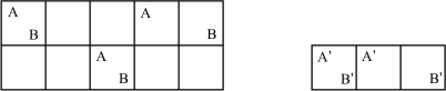
Figure 1: Comparison of facets in $\Delta_{5,2}^{1,2;\mathbf{1}}$.

For illustration let $A=(3,\{1,4\})$ and $B=(3,\{1,5\})$ be two facets of the complex $\Delta_{5,2}^{1,2;\mathbf{1}}$ (Figure 1 on the left). These two simplexes have the same element in the first row. Moreover the first column in the (lacunary) order (24) is empty for both $A$ and $B$ so it is the case (c) of the general comparison procedure that applies here. By removing the first row, the third column and the second (empty) column we obtain a $[3]\times[1]$ chessboard and the facets $A^{\prime}$ and $B^{\prime}$. This way the comparison of $A$ and $B$ is reduced to the comparison of $A^{\prime}$ and $B^{\prime}$ in $\Delta_{3,1}^{2;\mathbf{1}}$. The most natural choice is $A^{\prime}\ll B^{\prime}$ however (in light of Remark 4.5) we are free to choose any shelling order on $\Delta_{3,1}^{2;\mathbf{1}}$.

5 An application

The general colored Tverberg problem, as outlined in Sections 1.1 and 1.2, is the question of describing conditions which guarantee the existence of large intersecting families of multicolored (rainbow) simplices. By definition a simplex is multicolored if no two vertices are colored by the same color.

We can modify the problem by allowing multicolored simplices to contain not more than $p$ points of each color where $p\geq 1$ is prescribed in advance. Following the usual scheme (Section 1.3) we arrive at the generalized chessboard complexes $\Delta_{t,r}^{p,1}$.

This connection was one of the reasons why we were interested in the connectivity properties of multiple chessboard complexes $\Delta_{t,r}^{p,1}$ and the following statements illustrate some of possible applications. Further development of these ideas and new applications to Tverberg-van Kampen-Flores type theorems can be found in [JVZ-2].

Theorem 5.1

Let $r=p^{\alpha}$ be a prime power. Given $k$ finite sets of points in $\mathbb{R}^{d}$ (called colors), of $(p+1)r-1$ points each, so that $prk\geq(r-1)(d+1)+1$, it is possible to divide the points in $r$ groups with at most $p$ points of the same color in each group so that their convex hulls intersect.

Proof: The multicolored simplices are encoded as the simplices of the simplicial complex $([\ast]_{\Delta(p+1)}^{*((p+1)r-1)})^{*k}$. Indeed these are precisely the simplices which are allowed to have at most $p$ vertices in each of $k$ different colors. The configuration space of all $r$-tuples of disjoint multicolored simplices is the simplicial complex,

$$K=(([\ast]_{\Delta(p+1)}^{*((p+1)r-1)})^{*k})_{\Delta(2)}^{*r}.$$

Since the join and deleted join commute, this complex is isomorphic to,

$$K=(([\ast]_{\Delta(p+1)}^{*((p+1)r-1)})_{\Delta(2)}^{*r})^{*k}.$$

If we suppose, contrary to the statement of the theorem, that the intersection of images of any $r$ disjoint multicolored simplices is empty, the associated mapping $F:K\rightarrow(\mathbb{R}^{d})^{*r}$ would miss the diagonal $\Delta$. By composing this map with the orthogonal projection to $\Delta^{\perp}$, and after the radial projection to the unit sphere in $\Delta^{\perp}$, we obtain a $(\mathbb{Z}/p)^{\alpha}$-equivariant mapping,

$$\tilde{F}:K\rightarrow S^{(r-1)(d+1)-1}.$$

By Corollary 3.3, the complex $([\ast]_{\Delta(p+1)}^{*((p+1)r-1)})_{\Delta(2)}^{*r}$ is $(pr-2)$-connected, hence the complex $K$ is $(prk-2)$-connected. By our assumption $prk-2\geq(r-1)(d+1)-1$, so in light of Dold’s theorem [M03] such a mapping $\tilde{F}$ does not exist. $\square$

Specializing to the case $pk=d+1$, it is easy to see that we could take $(p+1)r-1$ points of each of $k$ colors in $\mathbb{R}^{pk-1}$ and obtain the following.

Corollary 5.2

Let $r$ be a prime power. Given $k$ finite sets of points in $\mathbb{R}^{pk-1}$ (called colors), of $(p+1)r-1$ points each, it is possible to divide the points in $r$ groups with at most $p$ points of the same color in each group so that their convex hulls intersect.

Of course, the continuous (non-linear) versions of the above results are true as well, and with the same proof.

If $r+1$ is a prime, there is a simple proof of this corollary using the result of [BMZ] which even obtains better estimate ($pr$ instead of $(p+1)r-1$) on the number of points of each color. Namely, one could divide each color of $pr$ points in $p$ ”subcolors” of $r$ points each, and obtain the desired division, even with some additional requirements on the points of the same color in each group. However, this argument works only in this case when $r+1$ is a prime.

Remark 5.3

A more general result related to Theorem 5.1 can be formulated if we allow each of $r$ multicolored sets to contain $p_{1}$ points of the first color, $p_{2}$ points of the second color, etc. $p_{k}$ points of the $k$-th color. In this case we arrive at the complex $\Delta_{t,r}^{p_{1},...,p_{k};{\mathbf{1}}}$ and its connectivity properties established by Theorem 3.2 can be used again. We omit the details since our main goal in this paper was to establish improved bounds on the connectivity of generalized chessboard complexes and Theorem 5.1 was useful to illustrate their importance and to show how they naturally appear in different mathematical contexts.

References

- [A04] C. Athanasiadis, Decompositions and connectivity of matching and chessboard complexes, Discrete Comput. Geom. 31 (2004), 395 -403.
- [BL] I. Bárány, D.G. Larman. A colored version of Tverberg’s theorem. J. London Math. Soc., II. Ser., 45:314–320, 1992.
- [BSS] I. Bárány, S.B. Shlosman, and A. Szücs. On a topological generalization of a theorem of Tverberg. J. London Math. Soc., 23:158–164, 1981.
- [Bjö95] A. Björner. Topological methods. In R. Graham, M. Grötschel, and L. Lovász, editors, Handbook of combinatorics, pages 1819–1872. North Holland, Amsterdam, 1995.
- [BLVŽ] A. Björner, L. Lovász, S.T. Vrećica, and R.T. Živaljević. Chessboard complexes and matching complexes. J. London Math. Soc. (2), 49(1):25–39, 1994.
- [BFZ] P.V.M. Blagojević, F. Frick, G.M. Ziegler, Tverberg plus constraints, Bulletin of the London Mathematical Society, 2014, Vol. 46, 953–967.
- [BMZ] P.V.M. Blagojević, B. Matschke, G.M. Ziegler. Optimal bounds for the colored Tverberg problem. J. European Math. Soc., Vol. 17, Issue 4, 2015, pp. 739 -754.
- [BMZ-2] P.V.M. Blagojević, B. Matschke, G.M. Ziegler. Optimal bounds for a colorful Tverberg–Vrećica problem, Advances in Math., Vol. 226, 2011, 5198–5215; arXiv:0911.2692v2 [math.AT].
- [FH98] J. Friedman and P. Hanlon. On the Betti numbers of chessboard complexes. J. Algebraic Combin., 8:193 203, 1998.
- [G79] P. F. Garst. Cohen-Macaulay complexes and group actions. PhD thesis, University of Wisconsin-Madison, 1979.
- [JVZ-2] D. Jojić, S.T. Vrećica, R.T. Živaljević. Symmetric multiple chessboard complexes and a new theorem of Tverberg type, arXiv:1502.05290 [math.CO].
- [J08] J. Jonsson. Simplicial Complexes of Graphs. Lecture Notes in Mathematics, Vol. 1928, Springer 2008.
- [KRW] D.B. Karaguezian, V. Reiner, M.L. Wachs. Matching Complexes, Bounded Degree Graph Complexes, and Weight Spaces of GL -Complexes. Journal of Algebra 239:77–92, 2001.
- [Koz] D. Kozlov. Combinatorial Algebraic Topology. Springer 2008.
- [M03] J. Matoušek. Using the Borsuk-Ulam Theorem. Lectures on Topological Methods in Combinatorics and Geometry. Universitext, Springer-Verlag, Heidelberg, 2003.
- [SW07] J. Shareshian and M. L. Wachs. Torsion in the matching complex and chessboard complex. Adv. Math., 212(2):525 -570, 2007.
- [T66] H. Tverberg. A generalization of Radon’s theorem. J. London Math. Soc., 41:123–128, 1966.
- [VŽ94] S. Vrećica and R. Živaljević. New cases of the colored Tverberg theorem. In H. Barcelo and G. Kalai, editors, Jerusalem Combinatorics ’93, Contemporary Mathematics Vol. 178, pp. 325–334, A.M.S. 1994.
- [VŽ11] S. Vrećica, R. Živaljević. Chessboard complexes indomitable. J. Combin. Theory Ser. A, 118(7):2157–2166, 2011.
- [Zi94] G.M. Ziegler. Shellability of chessboard complexes. Israel J. Math. 1994, Vol. 87, 97–110.
- [Zi11] G.M. Ziegler. colored points in a plane. Notices of the A.M.S. Vol. 58 , Number 4, 550–557, 2011.
- [Ž96] R. Živaljević. User’s guide to equivariant methods in combinatorics. Publications de l’Institut Mathematique (Beograd), 59(73), 114–130, 1996.
- [Ž98] R. Živaljević. User’s guide to equivariant methods in combinatorics II. Publications de l’Institut Mathematique (Beograd), 64(78) 1998, 107–132.
- [Ž99] R. Živaljević. The Tverberg-Vrećica problem and the combinatorial geometry on vector bundles. Israel J. Math, 111:53 -76, 1999.
- [Ž04] R.T. Živaljević. Topological methods. Chapter 14 in Handbook of Discrete and Computational Geometry, J.E. Goodman, J. O’Rourke, eds, Chapman & Hall/CRC 2004, 305–330.
- [ŽV92] R.T. Živaljević and S.T. Vrećica. The colored Tverberg’s problem and complexes of injective functions. J. Combin. Theory Ser. A, 61(2):309–318, 1992.