Modeling the anomaly of surface number densities of galaxies on the Galactic extinction map due to their FIR emission contamination

Abstract

The most widely used Galactic extinction map (Schlegel et al., 1998, SFD) is constructed assuming that the observed FIR fluxes entirely come from the Galactic dust. According to the earlier suggestion by Yahata et al. (2007), we consider how far-infrared (FIR) emission of galaxies affects the SFD map. We first compute the surface number density of SDSS DR7 galaxies as a function of the $r$-band extinction, $A_{r,\rm SFD}$. We confirm that the surface densities of those galaxies positively correlate with $A_{r,\rm SFD}$ for $A_{r,\rm SFD}<0.1$, as first discovered by Yahata et al. (2007) for SDSS DR4 galaxies. Next we construct an analytic model to compute the surface density of galaxies taking account of the contamination of their FIR emission. We adopt a log-normal probability distribution for the ratio of $100\mu\mathrm{m}$ and $r$-band luminosities of each galaxy, $y\equiv(\nu L)_{100\mu\mathrm{m}}/(\nu L)_{r}$. Then we search for the mean and r.m.s values of $y$ that fit the observed anomaly using the analytic model. The required values to reproduce the anomaly are roughly consistent with those measured from the stacking analysis of SDSS galaxies (Kashiwagi, Yahata, & Suto, 2013). Due to the limitation of our statistical modeling, we are not yet able to remove the FIR contamination of galaxies from the extinction map. Nevertheless the agreement with the model prediction suggests that the FIR emission of galaxies is mainly responsible for the observed anomaly. While the corresponding systematic error in the Galactic extinction map is 0.1 to 1mmag, it is directly correlated with galaxy clustering, and thus needs to be carefully examined in precision cosmology.

1. Introduction

The Galactic extinction map is the most fundamental data for astronomy and cosmology, since all extragalactic astronomical observations are inevitably conducted through the Galactic foreground, thus affected by the Galactic interstellar dust. In particular, lights in optical and ultraviolet bands are dimmed by the absorption and scattering of the Galactic dust. Therefore, we cannot determine any fundamental quantities such as intrinsic luminosities or colors of extragalactic objects without proper correction for the dust extinction. This is why the Galactic extinction correction could be one of the most critical sources of systematics.

The most widely-used Galactic extinction map was constructed by Schlegel et al. (1998, hereafter SFD) based on the IRAS/ISSA and COBE/DIRBE Far-infrared (FIR) emission maps, which are dominated by thermal dust emission. The construction of the SFD map consists of the following procedures:

1. constructing a dust temperature map from the ratio of the 100 $\mu\mathrm{m}$ flux to the 240 $\mu\mathrm{m}$ flux measured by DIRBE, which has $1^{\circ}.1$ FWHM spatial resolution,

2. calibrating the ISSA 100 $\mu\mathrm{m}$ emission map, which has the resolution of $6^{\prime}.1$ FWHM, according to the DIRBE 100 $\mu\mathrm{m}$ map,

3. correcting the calibrated ISSA 100 $\mu\mathrm{m}$ map for dust temperature using the previous temperature map,

4. converting the ISSA 100 $\mu\mathrm{m}$ map to color excess, $E(B-V)$, assuming the proportionality between the temperature corrected 100 $\mu\mathrm{m}$ flux, $I_{100\mu\mathrm{m}}$, and the dust column density:

   $$E(B-V)=pI_{100\mu\mathrm{m}}X(T),$$ (1)

   where $p$ is a constant determined from Mg${{\rm II}}$ indices of elliptical galaxies as standard color indicators, and $X(T)$ is the correction for the dust temperature.

The SFD map has achieved significant improvement in precision and resolution compared to the previous extinction maps constructed from H I 21-${\mathrm{cm}}$ emission (Burstein & Heiles, 1978, 1982). Nevertheless, it should be noted that the map is not based on any direct measurement of the dust absorption, but derived from its emission. Indeed one needs several assumptions to convert the FIR emission map into the extinction map. This is why it is important to test the reliability of the SFD map by comparing with other independent observations.

In high-extinction regions, such as molecular clouds or near the Galactic plane, many earlier studies examined the SFD map using star counts, NIR galaxy colors, and galaxy number counts (Arce & Goodman, 1999a, b; Chen et al., 1999; Cambrésy et al., 2001, 2005; Dobashi et al., 2005; Yasuda et al., 2007; Rowles & Froebrich, 2009). They often report that the SFD map over-predicts extinction in the high-extinction regions, possibly because of the poor angular resolution of the dust temperature map (Arce & Goodman, 1999a, b) and/or the existence of cold dust components with high emissivity in FIR.

In contrast, its reliability in low-extinction regions has not been carefully examined until recently. The Sloan Digital Sky Survey (SDSS; York et al., 2000) with very accurate photometry makes it possible to investigate the reliability of the SFD map even in those regions. Fukugita et al. (2004) tested the region of $E(B-V)<0.15$ in the SFD map on the basis of number counts of the SDSS DR1 (Abazajian et al., 2003) galaxies, and concluded that the SFD map prediction is consistent with the number counts. More recently, Schlafly et al. (2010) measured the dust reddening from the displacement of the bluer edge of the SDSS stellar locus, and found that the SFD map over-predicts dust reddening by $\sim$ 14% in $E(B-V)$. They also found that the extinction curve of the Galactic dust is better described by the Fitzpatrick (1999) reddening law rather than that of O’Donnell (1994). These results are also confirmed by an independent method (Schlafly & Finkbeiner, 2011). Peek & Graves (2010, hereafter PG) measured the dust reddening using the passively evolving galaxies as color standards and found that the SFD map under-predicts reddening where the dust temperature is low, but at most by 0.045 mag in $E(B-V)$. They provided the correction map for the SFD with $4^{\circ}.5$ resolution.

A systematic test of the SFD map was also performed by Yahata et al. (2007). They computed the surface number densities of the SDSS DR4 (Adelman-McCarthy et al., 2006) photometric galaxies as a function of the extinction. They found that the surface number densities of the SDSS galaxies exhibit a clear positive correlation with the SFD extinction in the low extinction region, $A_{r}<0.1$. They proposed that the observed FIR intensity, $I_{100\mu\mathrm{m}}$, is partially contaminated by the emission of galaxies along their direction. Since SFD compute the extinction assuming that the flux is entirely due to the Galactic dust, the region of more galaxies, therefore with stronger FIR intensity, is assigned a higher extinction. If the over-estimated extinction is applied, the corrected surface number density of galaxies becomes even higher than the real, resulting in the positive correlation with the extinction as observed. Yahata et al. (2007) performed a simple numerical experiment and showed that even a quite small contamination of FIR emission of galaxies could qualitatively reproduce the observed anomaly. Indeed the expected FIR emission was unambiguously discovered by the subsequent stacking image analysis of SDSS galaxies (Kashiwagi, Yahata, & Suto, 2013).

The main purpose of the present paper is to reproduce quantitatively the observed anomaly of the surface number density of SDSS galaxies on the SFD map by an analytic model of the contamination due to their FIR emission.

The rest of the paper is organized as follows; after the brief summary of the SDSS DR7 data (Abazajian et al., 2009) that we use here (§3), we repeat the surface number density analysis of galaxies introduced by Yahata et al. (2007). Section 4 performs mock numerical simulations so as to predict the surface number densities of galaxies by taking account of the effect of their FIR contamination. We also develop an analytic model, and make sure that it reproduces well the result of the Mock simulation in §5. The detailed description of our analytic model is presented in Appendix B. We perform the fit to the observed anomaly in the SFD map and find the mean of the $100\mu\mathrm{m}$ to $r$-band luminosity ratio, $y=(\nu L)_{100\mu\mathrm{m}}/(\nu L)_{r}$ per SDSS galaxy, is required to be $y_{\rm avg}>4$. Section 7 discusses the effect of the spatial clustering of galaxies, which is neglected either in mock simulations or in the analytic model. We also compare the optimal value of the $100\mu\mathrm{m}$ to $r$-band flux ratio with that independently derived with the stacking image analysis by Kashiwagi, Yahata, & Suto (2013). Similar analysis for the corrected SFD map according to Peek & Graves (2010) is also briefly mentioned. Finally §8 is devoted to summary and conclusions of the present paper.

2. The Sloan Digital Sky Survey DR7

The SDSS DR7 photometric observation covers 11663 $\rm{deg}^{2}$ of sky area, and collects 357 million objects with photometry in five passbands; $u$, $g$, $r$, $i$, and $z$ (For more details of the photometric data, see Gunn et al., 1998, 2006; Fukugita et al., 1996; Hogg et al., 2001; Ivezić et al., 2004; Smith et al., 2002; Tucker et al., 2006; Padmanabhan et al., 2008; Pier et al., 2003). The SDSS photometric data are corrected for the Galactic extinction according to the SFD map (Stoughton et al., 2002). They adopt the conversion factors from color excess to the dust extinction in each passband:

$$k_{x}\equiv\frac{A_{x,{\mathrm{SFD}}}}{{E(B-V)}},$$ (2)

where $x=u$, $g$, $r$, $i$, and $z$ (Table 6 of SFD). These factors are computed assuming the spectral energy density of an elliptical galaxy, and the reddening law of O’Donnell (1994) combined with the extinction curve parameter:

$$R_{V}\equiv\frac{A_{V}}{{E(B-V)}}=3.1.$$ (3)

The spatial distribution of stellar objects in the SDSS catalogue is likely to be correlated with the dust distribution. Therefore the reliable star-galaxy separation is critical for our present purpose of testing the SFD map from the distribution of extragalactic objects. We carefully construct a reliable photometric galaxy sample as follows.

2.1. Sky area selection

We choose the regions of SDSS DR7 survey area labeled “PRIMARY”. Indeed we found that the “PRIMARY” regions in the southern Galactic hemisphere are slightly different from the area where the objects are actually located. We are not able to understand why, and thus decide to use the regions in the northern Galactic hemisphere alone to avoid possible problems.

To ensure the quality of good photometric data, we exclude masked regions. The SDSS pipeline defines the five types of masked regions according to the observational conditions. We remove the four types of the masked regions, labeled “BLEEDING”, “BRIGHT$\_$STAR”, “TRAIL” and “HOLE” from our analysis. The masked regions labeled “SEEING” is not removed, since relatively bad seeing does not seriously affect the photometry of relatively bright galaxies that we use in the present analysis. The total area of the removed masked regions is about $340~{}\rm{deg}^{2}$, which comprises roughly $4.5\%$ of the entire “PRIMARY” regions in the northern Galactic hemisphere.

2.2. Removing false objects

We remove false objects according to photometry processing flags. We first remove fast-moving objects, which are likely the Solar System objects. We also discard objects that have bad photometry or were observed in the poor condition. A fraction of objects suffers from deblending problems, i.e., the decomposition of photometry images consisting of superimposed multi-objects is unreliable or failed. We remove such objects as well.

2.3. Magnitude range of galaxies

The SDSS catalogue defines the type of objects according to the differences between the cmodel and PSF magnitudes, where the former magnitude is computed from the composite flux of the linear combination of the best-fit exponential and de Vaucouleurs profiles.

Since the reliability of star-galaxy separation depends on the model magnitude before extinction correction, we must carefully choose the magnitude ranges of our sample for the analysis. In $r$-band, the star-galaxy separation is known to be reliable for galaxies brighter than $\sim$21 mag (Yasuda et al., 2001; Stoughton et al., 2002), while the saturation of stellar images typically occurs for objects brighter than 15 mag in $r$-band. Therefore, we choose the magnitude range conservatively as $17.5<m_{r}<19.4$, where $m_{r}$ denotes the observed (extinction uncorrected) magnitudes in $r$-band.

We adopt the same value of upper/lower limits for extinction corrected magnitudes. Figure 1 shows the differential number counts of SDSS galaxies as a function of $m_{x}$ for each bandpass. The faint-end threshold of our $r$-band selected sample, $m_{r}=19.4$, is $\sim 2$ mag brighter than the turnover of the differential number count. We similarly determine the faint-end of magnitude range for all bandpasses as 2 mag brighter than the turnover magnitude. We confirmed that shifting the upper or lower limits by $\pm 1.0$mag does not significantly change our conclusions below. We summarize the magnitude range and the number of galaxies with and without photometry flag selection for each bandpass in Table 1.

Figure 1.— Differential number counts of the photometric galaxy sample as functions of extinction uncorrected magnitudes for each band (solid lines). The vertical dashed lines indicate the magnitude ranges within which we use for the analysis.

Table 1The magnitude range and the number of SDSS galaxies for each bandpass. The third column shows the number of all SDSS galaxies within the magnitude range. The fourth column shows the number of the galaxies after photometry flag selection described in §2.2, which are used in our measurement in §3. The numbers of galaxies are counted without extinction correction.

bandpass	magnitude range	# of galaxies	# of galaxies	rejection rate
		(w/o flag selection)	(w/ flag selection)
$u$	$18.3<m_{u}<20.2$	1200586	633319	0.472
$g$	$18.0<m_{g}<20.4$	4891030	3428064	0.299
$r$	$17.5<m_{r}<19.4$	4347881	3205638	0.263
$i$	$17.0<m_{i}<18.9$	4450724	3140684	0.295
$z$	$16.8<m_{z}<18.3$	2984104	2136639	0.284

3. Surface number densities of SDSS DR7 photometric galaxies

3.1. Methodology

In this section, we extend the previous analysis of Yahata et al. (2007), and re-examine the anomaly in the surface number density of galaxies using the SDSS DR7 photometric galaxies, instead of DR4. The left panel of Figure 2 plots the sky area of the SDSS DR7 that is employed in our analysis, where the color scale indicates the value of the $r$-band extinction provided by SFD, $A_{r,{\mathrm{SFD}}}$.

Since most of the increased survey area of DR7 relative to DR4 corresponds to regions with $A_{r,\mathrm{SFD}}<0.1$mag, we can study the anomaly in such low-extinction regions discovered by Yahata et al. (2007) with higher statistical significance.

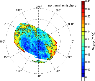
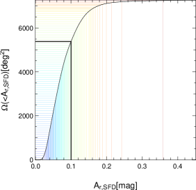
Figure 2.— Photometric survey area of the SDSS DR7 in Galactic coordinates (Left), and the cumulative distribution of the area as a function of $A_{r,\rm{SFD}}$ (Right). The left panel is color-coded according to the value of $A_{r,\rm{SFD}}$. The thick lines in the both panels indicate $A_{r,\rm{SFD}}=0.1$mag, corresponding to 74 $\%$ of the entire survey. The thin lines correspond to each bin of 84 subregions color-coded as the same as the left panel.

We first divide the entire sky area of the SDSS DR7 (right panel of Fig.2) into 84 subregions according to the value of $A_{r,{\mathrm{SFD}}}$. Each subregion is chosen so as to have an approximately same area ($\sim 100\rm{deg}^{2}$), and consists of spatially separated (disjoint) small patches over the sky. The right panel of Figure 2 shows the cumulative area fraction of the sky as a function of $A_{r,{\mathrm{SFD}}}$. Note that approximately 74 % of the entire sky corresponds to $A_{r,{\mathrm{SFD}}}<0.1$mag, in which we are interested.

Next we count the number of galaxies with the specified range of $r$-band magnitude in each subregion (§2.3), and obtain their surface number densities as a function of the extinction. Since the spatial distribution of galaxies is expected to be homogeneous when averaged over a sufficiently large area, the surface number densities of galaxies should be constant, and should not correlate with the extinction. In other words, any systematic trend with respect to $A_{r,{\mathrm{SFD}}}$ should indicate to a problem of the SFD map.

3.2. Results

Figure 3 shows the surface number densities of galaxies, $S_{\rm{gal}}$, in the 84 subregions for the five passbands. The red filled circles indicate $S_{\rm{gal}}$ uncorrected for dust extinction, while the blue filled triangles are the results after extinction correction using the SFD map. Note that the surface number densities of galaxies in different passpands are plotted against their corresponding $r$-band extinction, $A_{r,{\mathrm{SFD}}}$.

Following Yahata et al. (2007) again, we estimate the statistical error of the surface number density, $\sigma_{S}^{2}$, as follows:

$$\frac{\sigma_{S}^{2}}{S^{2}}=\frac{1}{N}+\frac{1}{\Omega^{2}}\int_{\Omega}\int_{\Omega}w(\theta_{12})d\Omega_{1}d\Omega_{2},$$ (4)

where $N$ and $S$ denote the number and the surface number density of the galaxies in the subregion of area $\Omega$, and $w(\theta_{12})$ is the angular correlation function of galaxies with $\theta_{12}$ being the angular separation between two solid angle elements, $d\Omega_{1}$ and $d\Omega_{2}$. The first term in equation (4) denotes the Poisson noise, while the second term comes from galaxy clustering.

For definiteness, we adopt the double power-law model (Scranton et al., 2002; Fukugita et al., 2004) for $w(\theta_{12})$:

$$w(\theta_{12})=\cases{0.008(\theta_{12}/\rm{deg})^{-0.75}&$(\theta_{12}\leq 1\rm{deg})$\cr 0.008(\theta_{12}/\rm{deg})^{-2.1}&$(\theta_{12}>1\rm{deg})$\cr}.$$ (5)

Strictly speaking, the integration in the second term of equation (4) should be performed over a complex and disjoint shape of each subregion. For simplicity, however, we substitute the integration over a circular region whose area is equal to that of the actual subregion. Although this approximation may overestimate the true error, it does not affect our conclusion at all. For the typical values of $\Omega\sim 100\rm{deg}^{2}$ and $S\sim 480\rm{deg}^{-2}$, we find that the second term is larger by two orders of magnitude than the first Poisson-noise term.

Figure 3 suggests that the SFD correction works well in relatively high-extinction regions, i.e., $A_{r,{\mathrm{SFD}}}>0.1$; before corrected for extinction, the surface number density of galaxy, $S_{\rm{gal}}$, monotonically decreases against $A_{r,{\mathrm{SFD}}}$ as naturally expected. It becomes roughly constant within the statistical error after extinction correction.

In low-extinction regions ($A_{r,{\mathrm{SFD}}}<0.1$), however, the uncorrected $S_{\rm{gal}}$ increases with $A_{r,{\mathrm{SFD}}}$, which is opposite to the behavior expected from the Galactic dust extinction. The anomalous positive correlation between surface number densities and extinction is even more enhanced after the extinction correction. Apart from the slight quantitative differences, these results are consistent with the trend discovered for the SDSS DR4 by Yahata et al. (2007), especially for the positive correlations in $A_{r,\rm SFD}<0.1$.

Yahata et al. (2007) argued that the trend is due to the presence of the FIR emission of galaxies, which contaminates the 100 $\mu\mathrm{m}$ flux of IRAS that is conventionally ascribed to the Galactic dust entirely. Indeed their hypothesis is now directly confirmed by the stacking analysis of Kashiwagi, Yahata, & Suto (2013), who detected the unambiguous signature of FIR emission from SDSS galaxies in the SFD map. Our next task, therefore, is to ask if the detected nature of the FIR emission of galaxies by Kashiwagi, Yahata, & Suto (2013) properly accounts for the anomaly that we described here. In what follows, we consider the surface number density of the galaxies measured in $r$-band alone, simply because it is the central SDSS passband, and the result is equally applicable to the other passbands.

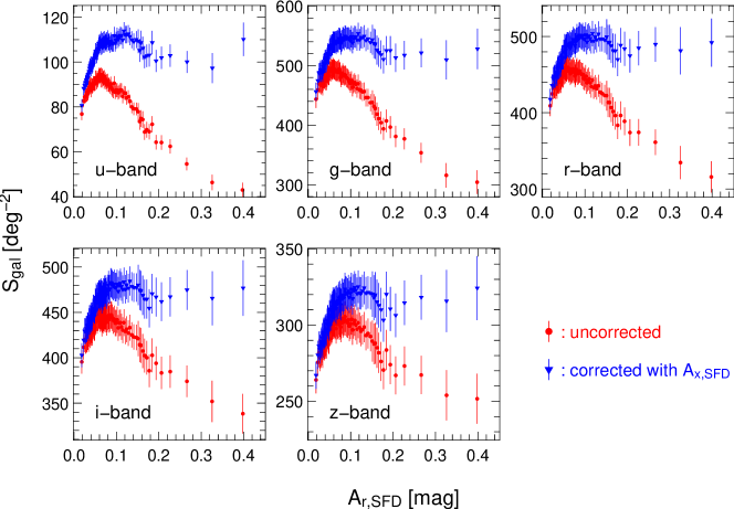
Figure 3.— Surface number densities of the SDSS DR7 photometric galaxy sample corresponding to Figure 1, against $A_{r,\mathrm{SFD}}$. The circles/triangles indicates the surface number densities calculated with extinction un-corrected/corrected magnitudes, respectively. The statistical errors are calculated from equation (4). The horizontal axis is the mean of $A_{r,{\mathrm{SFD}}}$ over the galaxies in each subregion.

4. Mock numerical simulation to compute the FIR contamination effect of galaxies on the extinction map

In this section, we present the results of mock numerical simulations that take into account the effect of the FIR emission of mock galaxies in a fairly straightforward manner. First we randomly place mock galaxies over the SDSS DR7 sky area so that they have the same number density and the same $r$-band magnitude distribution of the SDSS DR7 sample. Next, we assign a $100{\mu\mathrm{m}}$ flux to each mock galaxy according to the probability distribution function discussed in §4.1. We sum up the $100{\mu\mathrm{m}}$ fluxes of the mock galaxies over the raw SFD map that is assumed to be not contaminated by the FIR emission of mock galaxies, and construct a contaminated mock extinction map. Finally, we compute the surface number densities of mock galaxies exactly as we did for the real galaxy sample. Further details are described below.

4.1. Empirical correlation between 100$\mu$m and r-band luminosities of PSCz/SDSS galaxies

In order to assign 100$\mu\mathrm{m}$ emission to each mock galaxy with a given $r$-band magnitude, we need an empirical relation between the two luminosities, $L_{100\mu\mathrm{m}}$ and $L_{\rm r}$. For that purpose, Yahata (2007) created a sample of galaxies detected both in SDSS and in PSCz (IRAS Point Source Catalog Redshift Survey; Saunders et al., 2000). To be more specific, he searches for SDSS galaxies within 2 arcmin from the position of each PSCz galaxy, and selects the brightest one as the optical counterpart. Approximately 95% of the PSCz galaxies within the SDSS survey region have SDSS counterparts, and the resulting sample consists of 3304 galaxies in total. Note, however, that the sample is biased towards the FIR luminous galaxies since SDSS optical magnitude-limit is significantly deeper than that of PSCz galaxies.

Figure 4.— left panel; Relation between $\nu_{100\mu\rm{m}}L_{100\mu\rm{m}}$ and $\nu_{r}L_{r}$ for the PSCz/SDSS overlapped galaxies. right panel; same as the left panel, but for the mock galaxies generated based on $r$-band luminosity function (equation 13), the log-normal PDF of $y$ adopting the parameters in equation (21), and the flux cut $f_{\rm 100\mu\mathrm{m}}<1.0{\rm Jy}$.

The left panel of Figure 4 shows the relation between $\nu_{100\mu\rm{m}}L_{100\mu\rm{m}}$ (PSCz) and $\nu_{r}L_{r}$ (SDSS) of the PSCz/SDSS overlapped sample. For K-correction, we use the “K-corrections calculator” service (Chilingarian et al., 2010) for $r$-band, and extrapolate the FIR flux at 100$\mu\mathrm{m}$ from the second-order polynomials using 25 and 60 $\mu\mathrm{m}$ fluxes (Takeuchi et al., 2003).

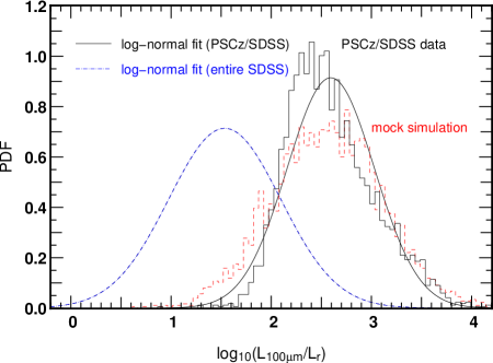
Figure 5.— The probability distribution function of $L_{100\mu\rm{m}}/L_{r}$; the PSCz/SDSS overlapped sample (histogram), the best-fit log-normal function (black solid curve), flux-limited mock galaxies (red dashed histogram), and the best-fit log-normal function estimated for the entire SDSS galaxies (blue dot dashed curve).

The resulting scatter plot indicates that $L_{100\mu\mathrm{m}}$ and $L_{r}$ are approximately proportional, albeit with considerable scatter. So we compute the probability distribution function (PDF) of the luminosity ratio,

$$y\equiv\frac{\nu_{100\mu\rm{m}}L_{100\mu\rm{m}}}{\nu_{r}L_{r}},$$ (6)

for the sample (solid histogram in Figure 5), and find that the PDF is reasonably well described by a log-normal distribution:

$$P_{\mathrm{ratio}}(y)dy=\frac{1}{y\ln 10\sqrt{2\pi\sigma^{2}}}\exp\left[-\frac{(\log_{10}y-\mu)^{2}}{2\sigma^{2}}\right]dy,$$ (7)

where $\mu=0.393$ and $\sigma=0.428$ are the mean and dispersion of $\log_{10}y$ (solid curve in Figure 5).

Since the PSCz/SDSS overlapped sample is a biased sample in a sense that these galaxies are selected towards the FIR luminous galaxies, the above log-normal distribution is not necessarily applicable for the entire SDSS galaxies. Therefore we assume the FIR-optical luminosity ratio of the entire SDSS galaxies also follows a log-normal distribution, and estimate the values of $\mu$ and $\sigma$ for the entire sample by considering the PSCz detection limit. Although the flux limit of PSCz is defined through $f_{60{\mu\mathrm{m}}}>0.6\rm{Jy}$, we roughly estimate the corresponding effective flux limit at 100$\mu\mathrm{m}$ is $f_{100{\mu\mathrm{m}}}>1.0\rm{Jy}$ from the distribution of $f_{100{\mu\mathrm{m}}}$ for the PSCz/SDSS galaxies (Left-panel of Figure 4).

Armed with these assumptions, the number of the galaxies that are detected by this flux cut and have the luminosity between $L_{r}\sim L_{r}+dL_{r}$ and $L_{100{\mu\mathrm{m}}}\sim L_{100{\mu\mathrm{m}}}+dL_{100{\mu\mathrm{m}}}$ is calculated as,

$$N^{\rm{obs}} ( L_{r},L_{100{\mu\mathrm{m}}})dL_{r}dL_{100{\mu\mathrm{m}}}$$ (8)

$$= \frac{\Omega_{s}}{4\pi}\bigg{[}\int^{\infty}_{0}dz\frac{dV(<z)}{dz}\Theta(L_{100{\mu\mathrm{m}}},z)$$ (10)

$$\times\Phi(L_{r})P(L_{100{\mu\mathrm{m}}}|L_{r};\mu,\sigma)\bigg{]}dL_{r}dL_{100{\mu\mathrm{m}}},$$

where $\Omega_{s}$ is the solid angle of the PSCz/SDSS overlapped survey area, and $V(<z)$ denotes the co-moving volume up to redshift $z$. The step function $\Theta(L_{100{\mu\mathrm{m}}},z)$ describes the flux cut of PSCz:

$$\Theta(L_{100{\mu\mathrm{m}}},z)=\cases{1&$(L_{100{\mu\mathrm{m}}}/4\pi d^{2}_{L}(z)>1.0{\rm Jy}$)\cr 0&$(\rm{else})$\cr},$$ (11)

where $d_{L}(z)$ is the luminosity distance at redshift $z$.

We adopt the double-Schechter luminosity function in $r$-band measured from the SDSS DR2 data (Blanton et al., 2005) for $\Phi(L_{r})$:

$$\Phi(L_{r})dL_{r} = \frac{dL_{r}}{L_{r,\ast}}\exp\left(-\frac{L_{r}}{L_{r,\ast}}\right)$$ (12)

$$\times \left[\phi_{\ast,1}\left(\frac{L_{r}}{L_{r,\ast}}\right)^{\alpha_{1}}+\phi_{\ast,2}\left(\frac{L_{r}}{L_{r,\ast}}\right)^{\alpha_{2}}\right].$$ (13)

The conditional probability density function of $L_{100{\mu\mathrm{m}}}$ for given $L_{r}$ is assumed to be log-normal:

$$P(L_{100{\mu\mathrm{m}}}|L_{r};\mu,\sigma)dL_{100{\mu\mathrm{m}}}=\frac{1}{\ln 10\sqrt{2\pi\sigma^{2}}}$$ (14)

$$\times \exp\left(-\frac{[\log(\nu_{100\mu\mathrm{m}}L_{100{\mu\mathrm{m}}}/\nu_{r}L_{r})-\mu]^{2}}{2\sigma^{2}}\right)\frac{dL_{100{\mu\mathrm{m}}}}{L_{100{\mu\mathrm{m}}}}$$ (15)

$$= yP_{\rm ratio}(y;\mu,\sigma)\frac{dL_{100\mu\mathrm{m}}}{L_{100\mu\mathrm{m}}}.$$ (16)

We use equation (10) to find the best-fit $\mu$ and $\sigma$ in equation (16) for the entire SDSS galaxies that reproduce the observed distribution of the PSCz/SDSS overlapped sample. The resulting values are $\mu=-0.662$ and $\sigma=0.559$ as plotted in blue dot-dashed line in Figure 5. This result indicates that the mean value of $y$ of the PSCz/SDSS overlapped sample is biased by an order of magnitude relative to that for the entire galaxies; see equation (20) and (21).

Adopting now the best-fit log-normal distribution, the luminosity function at $100{\mu\mathrm{m}}$ is calculated as

$$\Phi(L_{100{\mu\mathrm{m}}})=\int^{\infty}_{0}dL_{r}\Phi(L_{r})P(L_{100{\mu\mathrm{m}}}|L_{r};\mu,\sigma).$$ (17)

As plotted in Figure 6, the above best-fit indeed agrees well with the luminosity function independently measured from the PSCz data (Serjeant & Harrison, 2005).

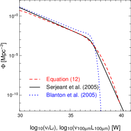
Figure 6.— Luminosity function (LF) of galaxies at $100\mu\mathrm{m}$ and $r$-band. Solid line is 100$\mu\mathrm{m}$ LF directly measured from the PSCz data (Serjeant & Harrison, 2005), while dashed line shows our estimate of 100$\mu\mathrm{m}$ LF based on equation (17) with the best-fit $\mu$, $\sigma$ and $r$-band LF (Blanton et al., 2005, blue dotted line).

In order to make sure if the above FIR log-normal PDF combined with the FIR flux cut reproduces the left panel of Figure 4, we generate mock galaxies and assign $z$, $L_{r}$, and $L_{100{\mu\mathrm{m}}}$ following the redshift distribution $dV(<z)$, and equations (13) and (16). Then we exclude those mock galaxies with $f_{100{\mu\mathrm{m}}}<1.0\rm{Jy}$ to mimic the flux cut. The right panel of Figure 4 and the dashed histogram in Figure 5 show the resulting luminosity distribution and the PDF of $y$ for those mock galaxies. Although not perfect, the mock galaxies reproduce the observed distribution reasonably well. We suspect that the discrepancy between the observed data and the mock simulation is mainly due to the limitation of our log-normal approximation neglecting the dependence of the ratio $L_{100{\mu\mathrm{m}}}/L_{60{\mu\mathrm{m}}}$ on $L_{100{\mu\mathrm{m}}}$.

For simplicity of the procedure, however, we adopt the best-fit log-normal distribution as the fiducial model of the 100 $\mu\mathrm{m}$ flux of the SDSS galaxies in what follows. In doing so, we parametrize the distribution by $y_{\rm avg}$ and $y_{\rm rms}$ instead of $\mu$ and $\sigma$:

$$y_{\rm avg} = e^{\mu\ln 10+(\sigma\ln 10)^{2}/2},$$ (18)

$$y_{\rm rms} = e^{\mu\ln 10+(\sigma\ln 10)^{2}/2}\sqrt{e^{(\sigma\ln 10)^{2}}-1},$$ (19)

since the anomaly is basically determined by $y_{\rm avg}$ as will be shown in Figure 9 below. For definiteness, the PSCz/SDSS overlapped sample is characterized by

$$\mu=0.393,\sigma=0.428,y_{\rm avg}=4.015,y_{\rm rms}=5.143,$$ (20)

while the entire SDSS sample is estimated to have

$$\mu=-0.662,\sigma=0.559,y_{\rm avg}=0.499,y_{\rm rms}=1.026.$$ (21)

4.2. Simulations

Now we are in a position to present our mock simulations that exhibit the effect of the FIR contamination of galaxies. In this subsection, we neglect the spatial clustering of galaxies and consider the case for Poisson distributed mock galaxies. The effect of spatial clustering of galaxies will be discussed separately in §7.1. Our mock simulations are performed as follows.

1. We distribute random particles as mock galaxies over the SDSS DR7 survey area. The number of the mock galaxies is adjusted so as to approximately match that of the SDSS photometric galaxies.

2. We assign an intrinsic apparent magnitude in $r$-band to each mock galaxy so that the resulting magnitude distribution reproduces that of the SDSS galaxies (Figure 1).

3. Assign $100\mu\mathrm{m}$ flux to each mock galaxy adopting the log-normal PDF for the $100\mu\mathrm{m}$-to-$r$-band flux ratio, $y$. The PDF is characterized by $y_{\rm avg}$ and $y_{\rm rms}$.

4. We convolve the $100{\mu\mathrm{m}}$ fluxes of the mock galaxies with a $\rm{FWHM}=5^{\prime}.2$ Gaussian filter, so as to mimic the SFD resolution, $\rm{FWHM}=6^{\prime}.1$ (see also Appendix A). Those mock galaxies with 100 $\mu\mathrm{m}$ flux being larger than $1.0\rm{Jy}$ are excluded, since SFD individually subtracted the 100$\mu\mathrm{m}$ emission of those bright galaxies. We include only the contribution of the mock galaxies with $17.5<m_{\rm r}<19.4$ so as to be consistent with our analysis in §3.2. We note, however, that in reality the FIR contamination would be likely contributed by galaxies outside the magnitude range (not only SDSS galaxies but non-SDSS galaxies that do not satisfy the SDSS selection criteria). Therefore the current mock simulation should be interpreted to see the extent to which the SDSS galaxies in that magnitude range alone account for the observed anomaly in their surface number density.

5. We superimpose the 100$\mu\mathrm{m}$ intensity of the mock galaxies on a true extinction map and construct a contaminated extinction map after subtracting the background (i.e., mean) level of the mock galaxy emission. In what follows, the resulting extinction with mock galaxy contaminated is denoted as $A_{r}^{\prime}$.

6. Finally, we calculate $S_{\rm{mock}}$, surface number densities of mock galaxies whose corrected/uncorrected magnitudes lie between 17.5 and 19.4 mag, repeating the same procedure discussed in §3, but using $A_{r}^{\prime}$ instead.

Note that our mock analysis uses the SFD map as the true extinction map without being contaminated by FIR emission of mock galaxies. Of course, the SFD map is contaminated by FIR emission from real galaxies, and thus cannot be regarded as a true extinction map for them. Nevertheless the contamination of real galaxies should not be correlated at all with the mock galaxies. This is why the SFD map can be used as the true extinction map for the current simulation.

The observed magnitude of each mock galaxy, i.e., affected by the Galactic dust absorption alone, is calculated from the true, in the present case the SFD map, but the extinction correction is done using $A^{\prime}_{r}$. Note that the difference between the true map and the contaminated map affects the value of extinction of regions where mock galaxies are located. Therefore, surface number densities of mock galaxies before the extinction correction are also influenced by the FIR contamination.

Figure 7 shows the surface number densities of mock galaxies as a function of $A_{r}^{\prime}$. Here we adopt $y_{\rm avg}=0.499$ and $y_{\rm rms}=1.026$, i.e., equation (21) which are estimated for the entire SDSS galaxy sample. The quoted error bars in the panel reflect the Poisson noise alone. The results exhibit a similar, but significantly weak correlation with $A_{r,{\rm SFD}}$ at $A_{r,{\rm SFD}}<0.1$ compared to the observed one (Fig.3), especially for the extinction-uncorrected surface densities.

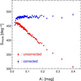
Figure 7.— The surface number densities of the randomly distributed mock galaxies with assigned magnitude of $17.5<m_{r}<19.4$. The symbols are the same as in Figure 3. The values of $y_{\rm avg}$ and $y_{\rm rms}$ estimated for the entire SDSS galaxies are adopted, instead of those for the PSCz/SDSS overlapped sample. The error bars reflect the Poisson noise alone.

Figure 8 would help us to understand the origin of the anomaly intuitively. (In this plot, we have adopted $y_{\rm avg}=10$ and $y_{\rm rms}=5$ just to clearly visualize the trends discussed in the following.) The dashed line indicates the differential distribution of the sky area as a function of $A_{r,\mathrm{SFD}}$, $\Omega(A_{r,\mathrm{SFD}})$, which corresponds to the derivative of the left panel of Figure 2. The black solid line shows the same distribution, but as a function of $A_{r}^{\prime}$. The resulting $\Omega^{\prime}(A^{\prime}_{r})$ slightly differs from $\Omega(A_{r,\mathrm{SFD}})$ due to the FIR contamination of mock galaxies.

The blue and red solid lines in Figure 8 show the differential number counts of galaxies, $N^{\prime}_{\rm gal,uncorr}$ and $N^{\prime}_{\rm gal,corr}$, as a function of $A_{r}^{\prime}$ calculated from magnitudes uncorrected/corrected for extinction with $A^{\prime}_{r}$. The shapes of $N^{\prime}_{\rm gal,uncorr}$ and $N^{\prime}_{\rm gal,corr}$ are slightly shifted towards the right relative to $\Omega^{\prime}(A_{r}^{\prime})$, because the pixels with more galaxies suffer from the larger contamination and thus have larger values of $A_{r}^{\prime}$.

Although the amount of this shift is quite small on average, the differences between $\Omega^{\prime}$ and the differential number counts for the same $A_{r}^{\prime}$ become larger in low-extinction regions because $\Omega^{\prime}$ is a rapidly increasing function of $A_{r}^{\prime}$. Therefore the surface number densities, $N^{\prime}_{\rm gal,uncorr}$ or $N^{\prime}_{\rm gal,corr}$ divided by $\Omega^{\prime}$, drastically change especially in low-extinction regions. In other words, the correlation between the surface number densities and $A_{r}^{\prime}$ is significantly enhanced due to the nature of the SDSS sky area and the SFD map. This also implies that the shape of the anomaly in $S_{\rm gal}$ is basically determined by the functional form of $\Omega(<A)$.

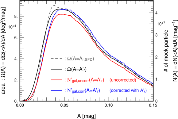
Figure 8.— The distribution of sky area and mock galaxies. The dashed line is the distribution of sky area as a function of true extinction, $A$, and the solid black line is calculated as a function of contaminated extinction, $A+\Delta A$. The red (blue) line indicates the distribution of number of galaxies as a function of contaminated extinction, $A+\Delta A$, with uncorrected (corrected) using the contaminated extinction. The distributions of number of galaxies are divided by the average surface number density, therefore surface number densities are equal to the average at the points where the distribution of sky area and number of galaxies cross. We have adopted $y_{\rm avg}=10$ and $y_{\rm rms}=5$ for clear visualization of the differences between each lines.

We also investigate how this result is affected by the $100\mu\mathrm{m}$ emission of galaxies outside the magnitude range. We incorporate the $100{\mu\mathrm{m}}$ flux of mock galaxies within a wider magnitude range ($15.0<m_{r}<21.0$), but the result is almost indistinguishable. This is mainly because that the additional contamination is not directly correlated with the surface number densities that we measure, partly because we neglect spatial clustering of galaxies. Therefore it affects only as the statistical noise in the extinction map, and does not contribute to the systematic correlation.

Finally we examine the dependence of the surface number densities on the parameters of $y_{\rm avg}$ and $y_{\mathrm{rms}}$ for log-normal PDF of $y$ (Fig. 9). The results indicate stronger correlations for larger $y_{\rm avg}$, but turn out to be relatively insensitive to $y_{\rm{rms}}$. This is why we choose $y_{\rm avg}$ and $y_{\rm rms}$, instead of $\mu$ and $\sigma$, to parametrize the log-normal PDF. A closer look reveals that larger $y_{\rm rms}$ shows slightly weaker anomaly, since a larger fraction of the mock galaxies are brighter than the IRAS/PSCz flux limit and does not contribute to FIR contamination. This effect of flux limit becomes critical for very large $y_{\rm avg}$ and $y_{\rm rms}$, as we will see in §6.1.

As seen above, the mock result adopting equation (21) estimated for the entire SDSS galaxies (Fig 7) indicates disagreement with the observed anomaly (Fig 3). This result may appear to imply that the hypothesis of galaxy FIR contamination fails to explain the observed anomaly. This is, however, not the case because we have neglected spatial clustering of galaxies. The previous parameters for the entire SDSS are estimated from the contribution of each single galaxy itself, but in the presence of galaxy clustering, the FIR emission associated with that galaxies can be significantly enhanced by the neighbor galaxies. In fact, the stacking analysis on the SFD map revealed that the FIR emission of neighbor galaxies dominate the central galaxy even by an order of magnitude (Kashiwagi, Yahata, & Suto, 2013). Therefore, we should adopt $y_{\rm avg}$ and $y_{\rm rms}$ that represent the total contribution both for each single galaxy and clustering neighbor galaxies, in order to reproduce the observed anomaly by our Poisson mock simulation.

In principle, we can probe such FIR fluxes from the comparison between mock simulations and observations, but the simulations are very time-consuming. Thus we develop an analytic model that reproduces the mock results in the next section.

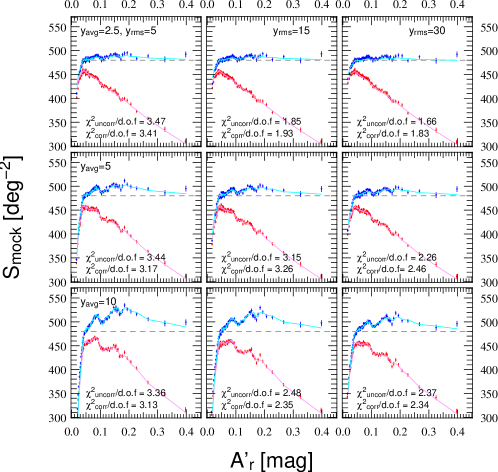
Figure 9.— The results of the mock simulations with Poisson distributed sample for various parameters of the log-normal PDF of $y$. The symbols indicate the results of the simulation for the mock Poisson sample, the same as Figure 7. The error bars reflect the Poisson noise alone. The cyan and pink lines indicate the analytic model prediction from equations (26) and (27) in §5. The lines and symbols are the same as Figure 7. The goodness of agreement between Poisson mock simulation and analytic model are evaluated by reduced $\chi^{2}$ for extinction un-corrected/corrected one, where only Poisson noise is considered. For all panels, the same average surface number density, $\bar{S}=480\mathrm{deg}^{-2}$, is assumed and shown as gray dashed lines.

5. Analytic model of the FIR contamination

In this section, we develop an analytic model that describes the anomaly of surface number densities of galaxies due to their FIR emission. The reliability of the analytic model is checked against the result of the numerical simulations presented in the previous section. We present a brief outline in the next subsection, and the details are described in Appendix B.

5.1. Outline

Let $A$ define the true Galactic extinction, not contaminated by the galaxy emissions. We denote the sky area whose value of the true extinction is between $A$ and $A+dA$ by $\Omega(A)dA$, and the number of galaxies that are located in the area $\Omega(A)dA$ by $N_{\mathrm{gal}}(A)dA$. Since there is no spatial correlation between galaxies and the Galactic dust, the corresponding surface number densities of the galaxies as a function of $A$:

$$S(A)\equiv\frac{N_{\mathrm{gal}}(A)}{\Omega(A)}$$ (22)

should be independent of $A$ and constant within the statistical error.

If the FIR emission from galaxies contaminates the true extinction, however, the above quantities should depend on the contaminated extinction, $A^{\prime}$, which are defined as $\Omega^{\prime}(A^{\prime})$ and $N^{\prime}_{\mathrm{gal}}(A^{\prime})$, respectively. Thus the observed surface number densities, $S^{\prime}(A^{\prime})$, should be

$$S^{\prime}(A^{\prime})=\frac{N_{\mathrm{gal}}^{\prime}(A^{\prime})}{\Omega^{\prime}(A^{\prime})}.$$ (23)

The essence of our analytic model is how to compute the expected $\Omega^{\prime}(A^{\prime})$ and $N_{\mathrm{gal}}^{\prime}(A^{\prime})$ under the presence of the FIR contamination of galaxies, which are distorted from the given true $\Omega(A)$ and $N_{\rm{gal}}(A)$.

Due to its angular resolution, the FIR emission of multiple galaxies contaminate to the extinction in the SFD map at a given position. Thus we need to sum up the FIR emission contribution of those galaxies located within the angular resolution scale:

$$A^{\prime}=A+\Delta A,$$ (24)

where the additional extinction, $\Delta A$, is computed by summing up the contribution of the $i$-th galaxies ($i=1\sim N$) located in the pixel:

$$\Delta A=\sum_{i=1}^{N}\Delta A_{i}.$$ (25)

In order to perform the summation analytically, we need a joint probability distribution function, $P_{\mathrm{joint}}(\Delta A,N)$, corresponding to the situation where there are $N$ galaxies in a pixel of the dust map, and the total contribution of those galaxies is $\Delta A$. In Appendix B, we present a prescription to compute $P_{\mathrm{joint}}(\Delta A,N)$, and provide the integral expressions for $\Omega^{\prime}(A^{\prime})$ and $N_{\mathrm{gal}}^{\prime}(A^{\prime})$.

5.2. Application of the analytic model

The analytic expressions for $\Omega^{\prime}(A^{\prime})$, $N^{\prime}_{\rm{gal,corr}}(A^{\prime})$ and $N^{\prime}_{\rm{gal,uncorr}}(A^{\prime})$ are given in equations (B8), (B21) and (B23) in Appendix B. Thus one can compute the surface number densities for the $i$-th subregion of the extinction between $A_{i}^{\prime}$ and $A_{i+1}^{\prime}$ as

$$S^{\prime}_{\rm{corr},i} = \frac{\int_{A_{i}^{\prime}}^{A_{i+1}^{\prime}}N^{\prime}_{\rm{gal,corr}}(A^{\prime})dA^{\prime}}{\int^{A_{i+1}^{\prime}}_{A_{i}^{\prime}}\Omega^{\prime}(A^{\prime})dA^{\prime}},$$ (26)

$$S^{\prime}_{\rm{uncorr},i} = \frac{\int_{A_{i}^{\prime}}^{A_{i+1}^{\prime}}N^{\prime}_{\rm{gal,uncorr}}(A^{\prime})dA^{\prime}}{\int^{A_{i+1}^{\prime}}_{A_{i}^{\prime}}\Omega^{\prime}(A^{\prime})dA^{\prime}},$$ (27)

where $S^{\prime}_{\rm{corr}}$ and $S^{\prime}_{\rm{uncorr}}$ are the extinction-corrected and uncorrected surface number densities, respectively. The solid lines in Figure 9 show the surface number densities calculated from equations (26) and (27) adopting 9 parameter sets of $y_{\rm avg}$ and $y_{\rm rms}$. The horizontal axis, an average extinction in each subregion, is calculated as

$$A^{\prime}_{\rm{corr},i} = \frac{\int_{A_{i}^{\prime}}^{A_{i+1}^{\prime}}A^{\prime}N^{\prime}_{\rm{gal,corr}}(A^{\prime})dA^{\prime}}{\int^{A_{i+1}^{\prime}}_{A_{i}^{\prime}}N^{\prime}_{\rm{gal,corr}}(A^{\prime})dA^{\prime}},$$ (28)

$$A^{\prime}_{\rm{uncorr},i} = \frac{\int_{A_{i}^{\prime}}^{A_{i+1}^{\prime}}A^{\prime}N^{\prime}_{\rm{gal,uncorr}}(A^{\prime})dA^{\prime}}{\int^{A_{i+1}^{\prime}}_{A_{i}^{\prime}}N^{\prime}_{\rm{gal,uncorr}}(A^{\prime})dA^{\prime}}.$$ (29)

Figure 9 clearly indicates that the analytic predictions and the simulation results are in good agreement. Strictly speaking, the agreement is not perfect in a sense that the reduced $\chi^{2}$ is as large as $\sim$ 3.5 for the worst cases, when only the Poisson noise is considered. The statistical errors for the observed SDSS surface number densities (Figure 3), however, includes the variance due to spatial clustering and are larger than the Poisson noise by an order of magnitude. Thus the discrepancy between the mock simulation and the analytic model is negligible for the parameter-fit analysis to the observational result in the following section.

6. Comparison of FIR contamination with the observed anomaly

Given the success of the analytic model described above, we compare the model prediction with the observed SFD anomaly. Our discussion in this section is organized as follows.

(1) We attempt to find the optimal values of $y_{\rm avg}$ and $y_{\rm rms}$ by fitting the analytic model prediction to the observed anomaly. It turns out that the observed anomaly is reproduced fairly well with a relatively wide range of $y_{\rm avg}$ and $y_{\rm rms}$ as long as $y_{\rm avg}$ is larger than $\sim 4$.

(2) This value of $y_{\rm avg}$ should be compared with with the empirical, and thus model-independent, result $y_{\rm avg}\approx 3.8$ obtained from the stacking analysis (Kashiwagi, Yahata, & Suto, 2013). The fact that the rough agreement of the two independent estimates for the average FIR to r-band fluxes is interpreted as a supporting evidence for our FIR explanation of the observed SFD anomaly.

(3) Finally, we attempt to reproduce the FIR flux of SDSS galaxies required above within our framework of the simplified modeling for FIR-to-optical relation. The estimated FIR flux qualitatively explains the result (2), but not quantitatively. We suspect that this is due to the limitation of our FIR assignment model for galaxies, and not the basic flaw of the FIR explanation for the SFD anomaly. Namely, given the fact that the stacking analysis already indicates the barely required value for $y_{\rm avg}$, we have to refine the FIR assignment model for SDSS galaxies, rather than to rule out the FIR explanation itself.

6.1. Estimating of the FIR emission of galaxies from the observed anomaly

Given the success of the analytic model described above, we attempt to find the best-fit parameters, $y_{\rm avg}$, and $y_{\mathrm{rms}}$, to the observed anomaly by minimizing

$$\chi^{2}(y_{\rm avg},y_{\mathrm{rms}},\bar{N})=\sum_{i}\frac{(S^{\rm{obs}}_{\rm{uncorr},i}-S^{\prime}_{\rm{uncorr},i})^{2}}{\sigma_{\rm{obs},i}^{2}},$$ (30)

where $S^{\rm{obs}}_{\rm{uncorr},i}$ is the extinction-uncorrected surface number densities in the $i$-th subregion of extinction, $\sigma_{\mathrm{obs},i}$ is its statistical errors, and $S^{\prime}_{\rm{uncorr},i}=S^{\prime}_{\rm{uncorr},i}(y_{\rm avg},y_{\mathrm{rms}},\bar{N})$ is the analytic model prediction given by equation (27). In the present fit, we use the extinction-uncorrected surface number densities, but the result is almost the same even if we use $S_{\rm{corr}}$ instead. In addition to $y_{\rm avg}$ and $y_{\rm rms}$, we include another free parameter, the intrinsic average number of galaxy in a pixel, $\bar{N}$, which is also unknown since the extinction correction is not necessarily reliable. It turns out that $\bar{N}$ is in the range of $480$ to $500\rm{[deg^{-2}]}$ and the results below is not sensitive to this value.

In reality, however, the resulting constraints are not so strong as shown in the top-left panel in Figure 10. This is partly due to the fact that we simply compute $\sigma_{\mathrm{obs},i}$ from the variance of each extinction bin, which does not represent the proper error. Thus our analysis here should be interpreted as a qualitative attempt to find a possible parameter space to explain the anomaly in terms of the FIR contamination; it would be quite difficult to make more quantitative analysis, given several crude approximations in our theoretical modeling and the poor angular-resolution and uncertain dust temperature correction in the SFD map.

Bearing this remark in mind, let us consider the constraints on $y_{\rm avg}$ – $y_{\rm{rms}}$ plane from the observed anomaly shown in the top-left panel of Figure 10. Fairly acceptable fits are obtained over the bluish region. Just for illustration, we select two widely separated points A and B with $(y_{\rm avg},y_{\rm rms})=(30,8000)$ and $(3.8,4.0)$, respectively, and plot the corresponding analytical predictions in the other three panels. Even though their $y_{\rm avg}$ is different by an order of magnitude, the two sets of parameters account for the observed anomaly reasonably and equally well.

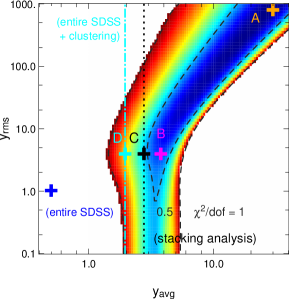
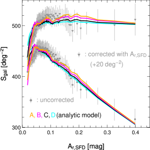
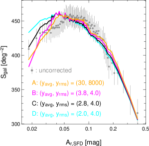
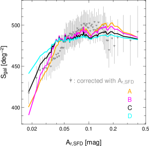
Figure 10.— Fit to the observed anomaly using the analytical model. top left panel; constraints on $y_{\rm avg}$ and $y_{\mathrm{rms}}$ through the chi-squared analysis with equation (30). The black dashed curves correspond to $\chi^{2}/{\rm d.o.f}=1$ and $\chi^{2}/{\rm d.o.f}=0.5$ constraints. The orange (A) and magenta (B) crosses are representative values that best explain the observed anomaly. The black dotted line and cross (C) indicates the value of $y_{\rm avg}$ estimated by stacking analysis (Kashiwagi, Yahata, & Suto, 2013). The blue cross shows the best-fit parameters for single galaxy of entire SDSS sample estimated in §4.1. The cyan dot-dashed line and cross (D) also indicates the value of $y_{\rm avg}$ estimated for entire SDSS sample, but including neighbor galaxies contribution (§6.3). top right panel; the analytic model predictions plotted over the observational data. The solid lines indicate the analytic prediction by equation (26) and (27), adopting the values of $(y_{\rm avg},y_{\rm rms})$ shown as the crosses in top left. The symbols are the observational results for the SDSS galaxies in $r$-band, the same as Figure 3. The plots for $S_{\rm gal}$ corrected with $A_{r,{\rm SFD}}$ are shifted by $+20{\rm deg}^{-2}$ just for clarity. bottom left; the same as top right, but indicates $S_{\rm gal}$ uncorrected for extinction and the horizontal axis is log-scaled. bottom left; the same as bottom left, but for $S_{\rm gal}$ corrected with $A_{r,{\rm SFD}}$.

6.2. Comparison with the stacking image analysis

We have shown that the anomaly in the surface number densities of SDSS galaxies on the SFD map is well reproduced by assuming their 100$\mu\mathrm{m}$ to $r$-band flux ratio is $\sim 3.8$ on average, where the 100$\mu\mathrm{m}$ flux includes the contribution of neighbor galaxies. On the other hand, the flux ratio of a single galaxy is estimated as $\sim 0.5$ (see §4.1).

Indeed these values should be compared with the result of the stacking image analysis by Kashiwagi, Yahata, & Suto (2013). They stacked the SDSS galaxies on the SFD map and found that a galaxy of $r$-band magnitude $m_{r}$ contributes to the extinction on average by

$$\Delta A_{r}^{\rm s}(m_{r})=0.087\times 10^{0.41(18-m_{r})}~{}{\rm[mmag]},$$ (31)

by itself (single term), and

$$\Delta A_{r}^{\rm tot}(m_{r})=0.64\times 10^{0.17(18-m_{r})}~{}{\rm[mmag]},$$ (32)

including the contribution from neighbor galaxies, corresponding to the clustering term in Kashiwagi, Yahata, & Suto (2013). The above extinction due to the $100\mu\mathrm{m}$ emission from galaxies is translated into its $100\mu\mathrm{m}$ to $r$-band flux ratio as

$$y=\frac{2\pi\sigma^{2}}{f_{r}\nu_{r}/\nu_{\rm 100\mu\mathrm{m}}}\frac{\Delta A_{r}}{k_{r}p},$$ (33)

where $\sigma$ is the Gaussian PSF width and $f_{r}$ is the $r$-band flux. Thus integrated over the differential number density, equations (31) and (32) suggest that

$$\bar{y}_{\rm avg}^{\rm s}=\frac{\int dm_{r}\frac{dN}{dm_{r}}y_{\rm avg}^{\rm s}(m_{r})}{\int dm_{r}\frac{dN}{dm_{r}}}=0.239,$$ (34)

and

$$\bar{y}_{\rm avg}^{\rm tot}=\frac{\int dm_{r}({dN}/{dm_{r}})y_{\rm avg}^{\rm c}(m_{r})}{\int dm_{r}({dN}/{dm_{r}})}=2.77,$$ (35)

respectively.

These values are based on the direct measurement of the FIR contamination, and thus independent of the modeling of 100$\mu\mathrm{m}$ to optical relation. We also emphasis that they should automatically include possible contributions from those galaxies not identified by SDSS. Therefore the sum of the two terms can be reliably interpreted as the expected contribution of the SDSS galaxies to $y_{\rm avg}$ including neighbor galaxies, which is plotted in Figure 10. While we do not know the corresponding $y_{\rm rms}$, we have already found that the dependence of the anomaly on $y_{\rm rms}$ is rather weak, at least in our analytic model. Thus the empirical value of $y_{\rm avg}$ from the stacking analysis roughly explains the observed anomaly as plotted in the three panels of Figure 10.

We interpret this agreement as a supporting evidence for the FIR model of the SFD anomaly given the fact that we assume a very simple relation between 100$\mu\mathrm{m}$ and optical luminosities, neglecting the galaxy morphology dependence that certainly leads to the FIR flux difference.

6.3. Estimates of clustering contribution of SDSS galaxies

We tried to independently estimate $y_{\rm avg}$, including an additional contribution of neighbor galaxies, using the SDSS galaxy distribution over the SFD map, instead of the stacking result by Kashiwagi, Yahata, & Suto (2013) discussed in §6.2. We first randomly assign the FIR flux of SDSS galaxies assuming $(y_{\rm avg},y_{\rm rms})=(0.5,1.0)$ for each SDSS galaxy itself neglecting the clustering term. Second, we sum up the FIR fluxes of galaxies convolved with the PSF of the SFD map (the Gaussian width of $3^{\prime}.1$) centered at each galaxy. Finally we compute $y_{\rm avg}$ and $y_{\rm rms}$ using the summed FIR fluxes after subtracting the average background flux.

Note that the resulting values of $y_{\rm avg}$ and $y_{\rm rms}$ should be diffrent from the above input values because of the contribution of the clustering term. We find $y_{\rm avg}\approx 2$, but $y_{\rm rms}$ is not well determined because it turned out to be very sensitive to the choice of the background flux. This result indicates that the FIR flux of the SDSS galaxies explains only a half of those required to well reproduce the observed anomaly, $y_{\rm avg}=3.8$.

Indeed, employing $y_{\rm avg}\approx 2$, our model still reproduces the anomaly qualitatively, but the predicted feature is substantially weaker than that of the observed one. The assigned FIR flux in this model, however, is based on the single galaxy contribution estimated in §4.1 ($y_{\rm avg}=0.5$), thus would be sensitive to the FIR assignment model. Given the fact that the empirical value from the stacking analysis, which is independent of such models, is fairly successful in reproducing the anomaly, we suspect that the factor of two difference originates from the limitation of our crude modeling for FIR flux, instead of the basic flaw of the FIR explanation of the anomaly.

7. Discussion

7.1. Effects of spatial clustering of galaxies

Both the mock simulations and the analytic model discussed in the previous section completely ignore the spatial clustering of galaxies. We, therefore, examine the clustering effect on the anomaly in this subsection. The most straightforward method is to replace the Poisson distributed mock galaxies by dark matter particles from cosmological N-body simulation. For that purpose, we use a realization in the standard $\Lambda\rm{CDM}$ cosmology with $\sigma_{8}=0.76$ performed by Nishimichi et al. (2009).

We repeat similar mock observations as discussed in §4.2, except for that we assign $r$-band luminosity to each mock galaxy instead of their apparent magnitude. To be specific, (i) we randomly assign $r$-band luminosities to all N-body dark matter particles according to the luminosity function of equation (13), (ii) convert their luminosities to apparent $r$-band magnitudes observed from a fixed observer position, and (iii) randomly select a fraction of the mock galaxies to match with the SDSS observed $dN/dm_{r}$ (Figure 1).

We repeat the same fitting analysis as Figure 10, except that the data are now replaced by the mock result on the basis of the cosmological N-body simulation with $y_{\rm avg}=3.8$ and $y_{\rm rms}=4.75$. The mock observation including the galaxy clustering effect result shows stronger anomaly than Poisson mock simulation with the identical $y_{\rm avg}$ and $y_{\rm rms}$. The analytic model that neglects the spatial clustering still reproduces the simulated anomaly very well, but the best-fit $y_{\rm avg}$ overestimate the real values employed in the simulation by a factor of $\sim$2. Thus the clustering effect can be absorbed effectively by re-interpreting the best-fit values of $y_{\rm avg}$ appropriately. The clustering effect estimated here is largely consistent with the clustering term contribution estimated directly from the SDSS galaxies (§6.3).

In order to quantitatively understand the relation between this bias and the strength of the galaxy spatial clustering, we have to incorporate the effect of spatial clustering in our analytic model. For that purpose, we measure the PDF of the number of the N-body mock particles in a pixel and replace the Poisson distribution in equation (B2) with the measured one. The analytic model prediction, however, hardly changes by such a modification. Thus more sophisticated improvements seem to be needed to account for the spatial clustering effect, which is beyond the scope of this paper.

7.2. Limitation of the correction for the FIR emission of galaxies

We attempt to correct the SFD map by subtracting the average FIR contamination of SDSS galaxies. The corrected extinction at an angular position $\mathbf{\theta}$ in the Galactic map is computed as

$$A_{r,{\rm corrected}}({\mathbf{\theta}})=A_{r,\rm SFD}({\mathbf{\theta}})-\sum_{j}\Delta A({\mathbf{\theta}_{j}-\mathbf{\theta}};m_{r}^{j}),$$ (36)

where ${\mathbf{\theta}_{j}}$ is the position of the $j$-th galaxy with its $r$-band magnitude of $m_{r}^{j}$. We employ 4 different values for $\Delta A$ given the uncertainty of the interpretation of the best-fit value of $y_{\rm avg}$ discussed before. As shown in Figure 11, however, the above correction does not seem to remove the anomaly so well. This results may imply that the dependence of FIR properties on galaxy population, which is neglected in our modeling, is essential for accurate correction for the FIR contamination. As a future work, such a morphology dependence of FIR luminosities of SDSS galaxies will be investigated by stacking analysis, especially using recent high resolution diffuse FIR measurements by AKARI (Murakami et al., 2007), WISE (Wright, 2010), etc.

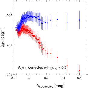
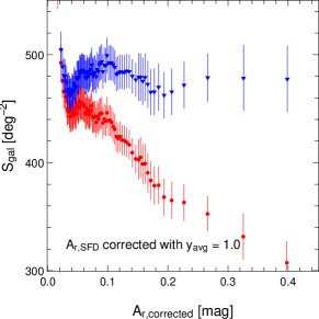
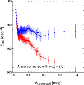
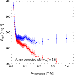
Figure 11.— Surface number densities of the SDSS galaxies with $17.5<m_{\rm r}<19.4$ after subtracting their average FIR emission contamination, where $y_{\rm avg}=0.3,1.0,2.0,3.8$ are adopted for estimation of the FIR emission of the SDSS galaxies.

7.3. Testing the Peek and Graves correction map

In §6.2, we found that the observed anomaly of the SDSS galaxies is roughly explained by the contamination of galaxy FIR emission. Nevertheless, the observed and predicted surface number densities (Fig 10) do not match perfectly, which might be attributed to other possible systematics in the SFD map.

In order to check the possible systematic effect, we use the improved extinction map by Peek & Graves (2010, hereafter PG). They found that the SFD map under-predicts extinction up to $\sim 0.1$ mag in $r$-band, using the passively evolving galaxies as standard color indicators. Their method is complementary to our galaxy number count analysis in a sense that they directly measure the reddening by the Galactic dust. Since the resolution of the PG correction map to SFD is $4^{\circ}.5$, the FIR fluctuations due to the emission of galaxies are not expected to be removed. The PG correction map, however, may have removed other systematics than the FIR contamination, which are not considered in our analytic model at all.

To see if their correction affect the number count analysis and the anomaly in the original SFD map, we repeat the same analysis described in §6 using the PG map. Basically, we find a very similar correlation between $S_{\rm gal}$ and $A_{r,\rm{PG}}$, suggesting that the PG map still suffers from the FIR contamination of galaxies as expected. We note, however, that our analytic model prediction exhibits slightly better agreement for the PG map than for the SFD map. This may indicates that possible systematic errors in the SFD map other than the FIR contamination is at least partially removed in the PG map.

8. Summary and conclusions

In the present paper, we have revisited the origin of the anomaly of surface number density of SDSS galaxies with respect to the Galactic extinction, originally pointed out by Yahata et al. (2007). We first computed the anomaly using the SDSS DR7 photometric catalogs, and then developed both numerical and analytic models to explain the anomaly. We take account of the contamination of galaxies in the IRAS $100{\mu\mathrm{m}}$ flux that was assumed to come entirely from the Galactic dust.

Our main findings are summarized as follows.

• Both numerical simulations and analytic model reproduce the observed anomaly quite well. Thus we quantitatively confirmed the validity of the hypothesis that the observed anomaly in the SFD Galactic extinction map is mainly due to the FIR emission from galaxies, originally proposed by Yahata et al. (2007).

• The comparison of the analytic model and the observed anomaly constrains mainly the average $100\mu\mathrm{m}$ to optical flux ratio for SDSS galaxies. The resulting value is in a reasonable agreement with that obtained from the stacking image analysis of the SDSS galaxies by Kashiwagi, Yahata, & Suto (2013).

• We also independently estimated the FIR contribution of single SDSS galaxy based on IRAS/SDSS overlapped catalogue data assuming a simple relation between FIR and optical luminosities. Summing up such FIR flux according to the SDSS galaxy distribution, however, we find that those contribution only explains roughly half of that required to reproduce the observed anomaly. This result may be due to the limitation of our modeling of the FIR to optical relation.

While our current analytic model still needs to be improved, the fact that the empirically determined value of $y_{\rm avg}$ nicely reproduces the observed anomaly indicates that the FIR emission of SDSS galaxies is the major origin of the anomaly.

In particular, we note that subtracting the average FIR contamination of the SDSS galaxies from the SFD extinction map does not properly remove the observed anomaly. This may imply that it is essential to consider the dependence of FIR emission on galaxy morphology and/or the effect of galaxy clustering, both of which we have neglected in the current analytical model. Since morphology and spatial clustering of galaxies are correlated in a complicated fashion, it is not easy to identify the good strategy of the correction method. We are currently working along this direction with the AKARI all-sky map data in $60,90,140,160\mu\mathrm{m}$. The stacking image analysis of SDSS galaxies with the higher-angular resolution map in multi-frequency bands would enable us to estimate the FIR emission of galaxies as a function of their properties including their color and morphology (T.Okabe et al. 2015, in preparation).

The FIR contamination that explains the anomalous behavior in the surface number density of the SDSS galaxies is just statistical and tiny, on the order of (0.1$\sim$1)mmag of extinction in $r$-band, which is much less serious than naively expected from the anomaly. Nevertheless the galaxy FIR emission is correlated with the large scale structure of the universe. Thus it may systematically bias the cosmological analysis. The present methodology is in principle applicable to check the reliability, and even to improve the accuracy of the future Galactic extinction map that should play a key role in all astronomical observations, in particular for the purpose of precision cosmology.

Appendix A Point Spread Function

In the mock simulation (§4), we assign the FIR fluxes to the mock galaxies by modeling the PDF of FIR to optical luminosity ratio, $y$. On the other hand, their contribution to the contamination in the SFD map is determined by their intensities as

$$\Delta A_{r}=pk_{r}\frac{f_{100\mu\mathrm{m}}}{2\pi\sigma^{2}_{\rm eff}},$$ (A1)

where $\sigma_{\rm eff}$ is the Gaussian width of the effective PSF, thus the impact of the FIR contamination directly depends on $\sigma_{\rm eff}$ even for the mock galaxies with the same $100\mu\mathrm{m}$ fluxes, $f_{100\mu\mathrm{m}}$. Due to the smoothing effects by the pixelization and interpolation of the SFD map, the effective PSF is degraded from that applied in the mock simulations (${\rm FWHM}=5^{\prime}.2$), which is aimed to mimic the purely instrumental PSF. Therefore, in order to precisely reproduce the mock simulation results by our analytic model (§5), we have to carefully evaluate the appropriate $\sigma_{\rm eff}$ to be applied in equation (B33). In this appendix, we derive $\sigma_{\rm eff}$ as a function of the intrinsic PSF width, $\sigma_{\rm int}$.

First we calculate the intensity of a single galaxy with a given $100\mu\mathrm{m}$ flux and position, taking into account of the two smoothing effects. Hereafter, we assume that the pixels of the SFD map are squares with the sides, $\theta_{\rm pix}=2^{\prime}.372$. We denote the pixel of the SFD map, in which the galaxy is located, as $\Omega_{0}$, and its neighbor pixels as $\Omega_{1}$ to $\Omega_{8}$. We define the 2-dimensional Cartesian coordinate system $\mathbf{\theta}=(\theta_{x},\theta_{y})$, whose origin is at the center of $\Omega_{0}$. The configuration of $\Omega_{0}$ to $\Omega_{8}$ is illustrated in the left panel of Figure 12. The intensity of the galaxy with $100\mu\mathrm{m}$ flux, $f$, in the pixel $\Omega_{i}$ ($i=0,...,8$) is given as

$$I_{i}(\mathbf{\theta}_{\rm g})=\frac{f}{2\pi\sigma_{\rm int}^{2}\Omega_{\rm pix}}\int_{\Omega_{i}}\exp\left(-\frac{|\mathbf{\theta}-\mathbf{\theta}_{\rm g}|^{2}}{2\sigma_{\rm int}^{2}}\right)d\mathbf{\theta},$$ (A2)

where $\mathbf{\theta}_{\rm g}$ denotes the position of the galaxy, and $\Omega_{\rm pix}=\theta_{\rm pix}^{2}$ is the area of the pixels. Since the value of the SFD map extinction is evaluated by the linear CIC interpolation, the intensity of the galaxy depends on $\theta_{\rm g}$, but also the position where the value is evaluated, $\theta$, and calculated as

$$I_{\rm{CIC}}(\mathbf{\theta},\mathbf{\theta}_{\rm g})=\left(1-\frac{\theta_{x}}{\theta_{\rm{pix}}}\right)\left(1-\frac{\theta_{y}}{\theta_{\rm{pix}}}\right) I {}_{i_{1}}(\mathbf{\theta}_{\rm g})+\left(1-\frac{\theta_{x}}{\theta_{\rm{pix}}}\right)\frac{\theta_{y}}{\theta_{\rm{pix}}}I_{i_{2}}(\mathbf{\theta}_{\rm g})$$ (A3)

$$+\frac{\theta_{x}}{\theta_{\rm{pix}}}\frac{\theta_{y}}{\theta_{\rm{pix}}} I {}_{i_{3}}(\mathbf{\theta}_{\rm g})+\frac{\theta_{x}}{\theta_{\rm{pix}}}\left(1-\frac{\theta_{y}}{\theta_{\rm{pix}}}\right)I_{i_{4}}(\mathbf{\theta}_{\rm g}),$$ (A4)

where $(i_{1},...,i_{4})$ are the indices of the nearest 4 pixels to $\theta$:

$$(\Omega_{i_{1}},\Omega_{i_{2}},\Omega_{i_{3}},\Omega_{i_{4}})=\cases{(\Omega_{0},\Omega_{1},\Omega_{2},\Omega_{3})&$(0<\theta_{x}<\frac{\theta_{\rm pix}}{2},0<\theta_{y}<\frac{\theta_{\rm pix}}{2})$\cr(\Omega_{0},\Omega_{5},\Omega_{4},\Omega_{3})&$(0<\theta_{x}<\frac{\theta_{\rm pix}}{2},-\frac{\theta_{\rm pix}}{2}<\theta_{y}<0)$\cr(\Omega_{0},\Omega_{5},\Omega_{6},\Omega_{7})&$(-\frac{\theta_{\rm pix}}{2}<\theta_{x}<0,-\frac{\theta_{\rm pix}}{2}<\theta_{y}<0)$\cr(\Omega_{0},\Omega_{1},\Omega_{8},\Omega_{7})&$(-\frac{\theta_{\rm pix}}{2}<\theta_{x}<0,0<\theta_{y}<\frac{\theta_{\rm pix}}{2})$\cr}.$$ (A5)

Since the resulting effective PSF also depends on $\theta$ and $\theta_{\rm g}$, we compute the PSF width appropriately averaged over $\theta$ and $\theta_{\rm g}$ in the following. In our analytic model (§5), we compute the expected $\Omega^{\prime}(A^{\prime})$ and $N^{\prime}_{\rm gal}(A^{\prime})$ under the presence of the FIR contamination of galaxies. We note that the effective PSF widths are slightly different for $\Omega^{\prime}(A^{\prime})$ and $N^{\prime}_{\rm gal}(A^{\prime})$. This is because the extinction contaminated by the FIR intensities, $A^{\prime}$, is always evaluated at the position of the galaxies, i.e., $\theta=\theta_{\rm g}$, for $N^{\prime}_{\rm gal}(A^{\prime})$, while this is not the case for $\Omega^{\prime}(A^{\prime})$. Therefore we separately derive the effective PSF widths for $\Omega^{\prime}(A^{\prime})$ and $N^{\prime}_{\rm gal}(A^{\prime})$. We denote these effective PSF widths as $\sigma_{{\rm eff},\Omega}$ and $\sigma_{{\rm eff},N}$.

Now let us calculate $\sigma_{{\rm eff},\Omega}$. Since $\theta$ and $\theta_{\rm g}$ are independent for computing $\Omega^{\prime}(A^{\prime})$, we calculate the intensity of galaxies averaged over $\theta$ and $\theta_{\rm g}$ as

$$\bar{I}=\frac{1}{\Omega_{\rm pix}^{2}}\int_{\Omega_{0}}d\mathbf{\theta}\int_{\Omega_{0}}d\mathbf{\theta}_{\rm g}I_{\rm{CIC}}(\mathbf{\theta},\mathbf{\theta}_{\rm g}).$$ (A6)

We define $\sigma_{{\rm eff},\Omega}$ as

$$\frac{f}{2\pi\sigma^{2}_{\rm{eff},\Omega}}\equiv\bar{I},$$ (A7)

and this leads to

$$\sigma_{{\rm eff},\Omega}=\frac{4}{\sqrt{\pi}}\frac{\Omega_{\rm pix}}{\sigma_{\rm int}}\frac{1}{6F(s)-5F(0)-2F(-s)+F(-2s)},$$ (A8)

where

$$F(x)=\int{\rm erf}(x)dx=x~{}{\rm erf}(x)+\frac{e^{-x^{2}}}{\sqrt{\pi}},$$ (A9)

$s=\theta_{\rm pix}/\sqrt{2}\sigma_{\rm int}$, and ${\rm erf}(x)$ denotes the error function.

Similarly, considering that $\theta=\theta_{\rm g}$, we define $\sigma_{{\rm eff},N}$ as

$$\frac{f}{2\pi\sigma^{2}_{{\rm eff},N}}\equiv\frac{1}{\Omega_{\rm pix}}\int_{\Omega_{0}}I_{\rm{CIC}}(\mathbf{\theta}_{\rm g},\mathbf{\theta}_{\rm g})d\mathbf{\theta}_{\rm g}.$$ (A10)

Equation (A10) is reduced to

$$\sigma_{{\rm eff},N}=\frac{\Omega_{\rm pix}}{\sqrt{8\pi\mathcal{R}}},$$ (A11)

where

$$\frac{2\mathcal{R}}{\sigma^{2}_{\rm int}}=\left[J_{1}\left(-\frac{\theta_{\rm pix}}{2}\right)-J_{2}\left(-\frac{\theta_{\rm pix}}{2}\right)\right]^{2}+2J_{1}\left(-\frac{\theta_{\rm pix}}{2}\right)J_{2}\left(\frac{\theta_{\rm pix}}{2}\right)-2J_{2}\left(-\frac{\theta_{\rm pix}}{2}\right)J_{2}\left(\frac{\theta_{\rm pix}}{2}\right)+J_{2}\left(\frac{\theta_{\rm pix}}{2}\right)J_{2}\left(\frac{\theta_{\rm pix}}{2}\right),$$ (A12)

$$J_{1}(x) = \left[F(b+s)-F\left(b+\frac{s}{2}\right)-F(b)+F\left(b-\frac{s}{2}\right)\right],$$ (A13)

$$J_{2}(x) = \frac{1}{s}\left[G(b+s)-G\left(b+\frac{s}{2}\right)-G(b)+G\left(b-\frac{s}{2}\right)\right]-\frac{1}{2}\left[F\left(b+\frac{s}{2}\right)-F\left(b-\frac{s}{2}\right)\right]$$ (A14)

$$+\frac{1}{2s}\left[{\rm erf}(b+s)-{\rm erf}\left(b+\frac{s}{2}\right)-{\rm erf}(b)+{\rm erf}\left(b-\frac{s}{2}\right)\right],$$ (A15)

$$G(x) = \int x~{}{\rm erf}(x)dx=\frac{1}{2}\left[x^{2}{\rm erf}(x)+\frac{1}{\sqrt{\pi}}xe^{-x^{2}}-\frac{1}{2}{\rm erf}(x)\right],$$ (A16)

and $b\equiv x/\sqrt{2}\sigma_{\rm int}$.

The right panel of Figure 12 shows the equations (A8) and (A11) as functions of $\sigma_{\rm int}$, which are adopted to equation (B33) in the analytic model presented in Appendix B. In numerical simulations in §4, we adopted $\sigma_{\rm int}=2^{\prime}.21$, which reproduces the effective resolutions $\sigma_{{\rm eff},\Omega}$ and $\sigma_{{\rm eff},N}$ both similar to the SFD angular resolution ${\rm FWHM}=6^{\prime}.1$.

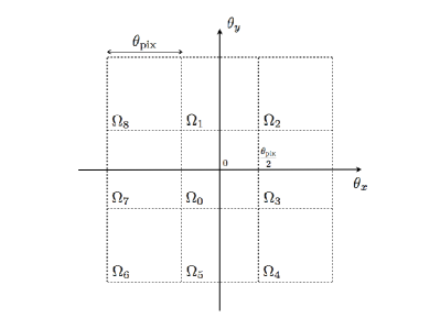
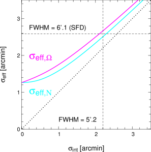
Figure 12.— left panel; Configuration of the SFD map pixels for calculating the effective PSF width. right panel; The effective Gaussian PSF widths, $\sigma_{{\rm eff},\Omega}$ (magenta) and $\sigma_{{\rm eff},N}$ (cyan), as functions of the intrinsic PSF width $\sigma_{\rm int}$. The vertical and horizontal dashed lines indicate the Gaussian PSF width applied in the mock simulation (§4), and the resolution of the SFD map, respectively.

Appendix B Analytic model neglecting spatial clustering of galaxies

Assume that galaxies are randomly distributed over the pixel, and denote the expected number of the galaxies of the true (albeit unobservable) apparent magnitude $m_{\rm true}$ being $m_{\rm min}<m_{\rm true}<m_{\rm max}$ by $\overline{N}$. Then the probability that the pixel has $N$ galaxies obeys the Poisson distribution:

$$P_{\rm{Poisson}}(N|\overline{N})=\frac{\overline{N}^{N}\exp(-\overline{N})}{N!}.$$ (B1)

Here we assume that the area of all the pixels of the dust map is equal. Then the joint probability is the product of the conditional probability that the total FIR contamination in the pixel is $\Delta A$, given that there are $N$ galaxies and that the probability that the pixel has $N$ galaxies:

$$P_{\rm{joint}}(\Delta A,N)=P_{N}(\Delta A)P_{\rm{Poisson}}(N|\overline{N}).$$ (B2)

The conditional probability $P_{N}(\Delta A)$ can be computed recursively. When there is no galaxy in a pixel ($N=0$), $\Delta A$ should vanish:

$$P_{0}(\Delta A)=\delta_{D}(\Delta A),$$ (B3)

where $\delta_{D}$ is the 1-dimensional Dirac delta function. We compute $P_{1}(\Delta A)$ from the differential number count of galaxy magnitude and the PDF of the FIR to $r$-band flux ratio as discussed later in detail. Then $P_{N}(\Delta A)$ for $N\geq 2$ should satisfy the following recursive equation:

$$P_{N}(\Delta A)=\int_{0}^{\Delta A}dxP_{1}(x)P_{N-1}(\Delta A-x).$$ (B4)

Finally the PDF of the total contamination in a pixel, $P(\Delta A)$, is given as

$$P(\Delta A) = \sum_{N=0}^{\infty}P_{\rm{joint}}(\Delta A,N)=\sum_{N=0}^{\infty}P_{N}(\Delta A)P_{\rm{Poisson}}(N|\overline{N}).$$ (B5)

Note therefore that $P_{\rm{joint}}(\Delta A,N)$ and $P(\Delta A)$ are computed in a straightforward fashion once the two inputs, $P_{1}(\Delta A)$ and $\overline{N}$, are specified from the observed data.

Next let us proceed to compute $\Omega^{\prime}(A^{\prime})$ and $N^{\prime}(A^{\prime})$ according to this model. Since SFD subtracted the mean FIR contamination in a pixel in constructing the map, we also subtract its theoretical counterpart:

$$\overline{\Delta A}=\int_{0}^{\infty}d(\Delta A)\Delta AP(\Delta A),$$ (B6)

from the FIR contamination $\Delta A$ in each pixel. So the extinction contaminated by the galaxy emission is now given by

$$A^{\prime}=A+\Delta A-\overline{\Delta A}.$$ (B7)

Therefore, the probability that a pixel with the true extinction $A$ is observed as $A^{\prime}$ due to the FIR contamination is given by $P(\Delta A)=P(A^{\prime}-A+\overline{\Delta A})$. Finally we obtain the expected observed distribution function of sky area, $\Omega^{\prime}(A^{\prime})$ as

$$\Omega^{\prime}(A^{\prime}) = \int_{0}^{\infty}dA\int_{0}^{\infty}d(\Delta A)\Omega(A)P(\Delta A)\delta_{D}\big{(}A^{\prime}-(A+\Delta A-\overline{\Delta A})\big{)}=\int_{0}^{A^{\prime}+\overline{\Delta A}}dA\Omega(A)P(A^{\prime}-A+\overline{\Delta A}).$$ (B8)

We can similarly derive the expression for $N_{\rm{gal}}^{\prime}(A^{\prime})$, the number distribution of the galaxies located in the pixels of the extinction $A^{\prime}$, as follows.

Since we assume that the area of each pixel is the same and equal to $\Omega_{\rm{pixel}}$, the number of pixels that have the true extinction in the range of $A$ and $A+dA$ is

$$N_{\rm{pixel}}(A)dA=\frac{\Omega(A)dA}{\Omega_{\rm{pixel}}}.$$ (B9)

Thus the expected number distribution of galaxies in a pixel that suffers from the FIR contamination of $\Delta A$ is

$$\overline{N}(\Delta A)=\sum_{N=0}^{\infty}NP_{\rm{joint}}(\Delta A,N).$$ (B10)

Therefore, the number distribution of galaxies, $N_{\rm{gal}}^{\prime}(A^{\prime})$, is given as

$$N_{\rm{gal}}^{\prime}(A^{\prime}) = \int_{0}^{\infty}dA\int_{0}^{\infty}d(\Delta A)N_{\rm{pixel}}(A)\overline{N}(\Delta A)\delta_{D}\big{(}A^{\prime}-(A+\Delta A-\overline{\Delta A})\big{)}$$ (B11)

$$= \int_{0}^{A^{\prime}+\overline{\Delta A}}d(\Delta A)N_{\rm{pixel}}(A^{\prime}-\Delta A+\overline{\Delta A})\overline{N}(\Delta A).$$ (B12)

While the above expression is correct for those galaxies with $m_{\rm min}<m_{\rm true}<m_{\rm max}$, we cannot measure their true magnitude $m_{\rm true}$ in reality, and one has to take into account the selection effect carefully. Consider a galaxy of $m_{\rm true}$ is located in a pixel of the contaminated extinction of $A^{\prime}$. Then its observed (uncorrected) magnitude is

$$m_{\rm uncorr}(A^{\prime})=m_{\rm true}+A,$$ (B13)

because its magnitude suffers from the true Galactic extinction $A$ alone, instead of $A^{\prime}$. This yields the corrected magnitude relying on the contaminated extinction $A^{\prime}$:

$$m_{\rm corr}(A^{\prime}) = m_{\rm uncorr}(A^{\prime})-A^{\prime}=m_{\rm true}+A-A^{\prime}=m_{\rm true}-(\Delta A-\overline{\Delta A})$$ (B14)

leading to the over-correction by the amount of $\Delta A-\overline{\Delta A}$.

Therefore, those galaxies with $m_{\rm min}<m_{\rm corr}(A^{\prime})<m_{\rm max}$ indeed correspond to

$$m_{\rm min}+(\Delta A-\overline{\Delta A})<m_{\rm true}<m_{\rm max}+(\Delta A-\overline{\Delta A}).$$ (B15)

In other words, the selection incorrectly excludes galaxies with $m_{\rm min}<m_{\rm true}<m_{\rm min}+\Delta A-\overline{\Delta A}$, and includes those with $m_{\rm max}<m_{\rm true}<m_{\rm max}+\Delta A-\overline{\Delta A}$ because of the contamination of FIR galaxy emission.

Given their differential number count with respect to magnitude, the number of such galaxies can be computed as

$$N_{\rm{ex,corr}}(\Delta A) = \int_{m_{\rm{min}}}^{m_{\rm{min}}+\Delta A-\overline{\Delta A}}\frac{dn(<m)}{dm}dm,$$ (B16)

$$N_{\rm{in,corr}}(\Delta A) = \int_{m_{\rm{max}}}^{m_{\rm{max}}+\Delta A-\overline{\Delta A}}\frac{d\overline{n}(<m)}{dm}dm.$$ (B17)

We adopt a power-law fit with a slope $\gamma$ (see Fig. 1) for the differential number counts of galaxies in a pixel that contains $N$ and $\overline{N}$ galaxies:

$$\frac{dn(<m)}{dm} = \frac{N\gamma 10^{\gamma m}\ln 10}{10^{\gamma m_{\rm{max}}}-10^{\gamma m_{\rm{min}}}},$$ (B18)

$$\frac{d\overline{n}(<m)}{dm} = \frac{\overline{N}\gamma 10^{\gamma m}\ln 10}{10^{\gamma m_{\rm{max}}}-10^{\gamma m_{\rm{min}}}}.$$ (B19)

The excluded number should be normalized for the actual number of galaxies, $N$, instead of $\overline{N}$, in the pixel. Nevertheless the included number is not correlated to $N$ in the Poisson distributed assumption, and thus should be normalized for $\overline{N}$.

Therefore we obtain finally the number distribution of galaxies after correcting for the contaminated extinction $A^{\prime}$ as

$$N_{\rm{gal,corr}}^{\prime}(A^{\prime}) = \int_{0}^{\infty}dA\int_{0}^{\infty}d(\Delta A)N_{\rm{pixel}}(A)[\overline{N}(\Delta A)-N_{\rm{ex,corr}}(\Delta A)+N_{\rm{in,corr}}(\Delta A)]\delta_{D}\big{(}A^{\prime}-(A+\Delta A-\overline{\Delta A})\big{)}$$ (B20)

$$= \int_{0}^{A^{\prime}+\overline{\Delta A}}d(\Delta A)N_{\rm{pixel}}(A^{\prime}-\Delta A+\overline{\Delta A})\times[\overline{N}(\Delta A)-N_{\rm{ex,corr}}(\Delta A)+N_{\rm{in,corr}}(\Delta A)].$$ (B21)

Similarly, the number distribution of galaxies before correcting for the contaminated extinction $A^{\prime}$, i.e., with $m_{\rm min}-A<m_{\rm true}<m_{\rm max}-A$, is given as

$$N_{\rm{gal,uncorr}}^{\prime}(A^{\prime}) = \int_{0}^{\infty}dA\int_{0}^{\infty}d(\Delta A)N_{\rm{pixel}}(A)[\overline{N}(\Delta A)-N_{\rm{ex,uncorr}}(A)+N_{\rm{in,uncorr}}(A)]$$ (B22)

$$\times \delta_{D}\big{(}A^{\prime}-(A+\Delta A-\overline{\Delta A})\big{)},$$ (B23)

where

$$N_{\rm{ex,uncorr}}(A)=\int_{m_{\rm{max}}-A}^{m_{\rm{max}}}\frac{dn(<m)}{dm}dm,$$ (B24)

and

$$N_{\rm{in,uncorr}}(A)=\int_{m_{\rm{min}}-A}^{m_{\rm{min}}}\frac{d\overline{n}(<m)}{dm}dm.$$ (B25)

In order to proceed further, we need an expression for the PDF of the FIR contamination due to a single galaxy, $P_{1}(\Delta A)$. The mock simulations presented in §4 convert the $r$-band magnitude, $m_{r}$, of each mock galaxy into its 100 ${\mu\mathrm{m}}$ flux from the FIR/optical luminosity ratio $y$ as

$$f_{100\mu\mathrm{m}}(m_{r},y)=yf_{0}10^{-0.4m_{r}},$$ (B26)

where $f_{0}=3631{\rm Jy}$, and $y$ is assumed to obey the log-normal PDF $P_{\rm{ratio}}$ given by equation (7). In the present analytic model, we further assume that the differential number count of galaxies in $r$-band obeys

$$P_{\rm{mag}}(m_{r})=\frac{\gamma_{r}10^{\gamma_{r}m_{r}}\ln 10}{10^{\gamma_{r}m_{r,\rm{max}}}-10^{\gamma_{r}m_{r,\rm{min}}}},$$ (B27)

where $m_{r,\rm{max}}$ and $m_{r,\rm{min}}$ denote the upper and lower limits of the magnitude, and $\gamma_{r}$ is the power-law index.

Once $P_{\rm{mag}}(m_{r})$ and $P_{\rm{ratio}}(y)$ are given, the PDF of 100$\mu\mathrm{m}$ flux from a single galaxy is computed as

$$P_{\rm flux}(f) = \int dy\int dm_{r}~{}P_{\rm{mag}}(m_{r})P_{\rm{ratio}}(y)\delta_{D}\big{(}f-f_{100{\mu\mathrm{m}}}(m_{r},y)\big{)}.$$ (B28)

With the PDFs of equations (B27) and (7), $P_{\rm flux}(f)$ reduces to

$$P_{\rm flux}(f) = K\left(\frac{f}{f_{0}}\right)^{-1-\frac{5}{2}\gamma_{r}}\left[\mathrm{erf}\big{(}s_{\rm{max}}(f)\big{)}-\mathrm{erf}\big{(}s_{\rm{min}}(f)\big{)}\right],$$ (B29)

where $\mathrm{erf}(x)$ denotes the error function, and $K$, $s_{\rm{max}}$ and $s_{\rm{min}}$ are defined as

$$K \equiv \frac{5\gamma_{r}10^{\frac{5}{2}\mu\gamma_{r}}}{4f_{0}(10^{\gamma_{r}m_{r,\rm{max}}}-10^{\gamma_{r}m_{r,\rm{min}}})}\exp\left[\frac{25}{8}\sigma^{2}\gamma_{r}^{2}(\ln 10)^{2}\right],$$ (B30)

$$s_{\rm{max}}(f) \equiv \frac{1}{\sqrt{2\sigma^{2}}}\bigg{[}0.4m_{r,\rm{max}}-\mu+\log_{10}\left(\frac{f}{f_{0}}\right)-\frac{5}{2}\sigma^{2}\gamma_{r}\ln 10\bigg{]},$$ (B31)

$$s_{\rm{min}}(f) \equiv \frac{1}{\sqrt{2\sigma^{2}}}\bigg{[}0.4m_{r,\rm{min}}-\mu+\log_{10}\left(\frac{f}{f_{0}}\right)-\frac{5}{2}\sigma^{2}\gamma_{r}\ln 10\bigg{]}.$$ (B32)

Incidentally, $P_{\rm flux}(f)$ turns out to be well approximated by a log-normal function also, but we use equation (B29) to be precise. Considering that the mock galaxies with flux larger than $f_{\rm lim}$ are removed and do not contaminate, $P_{1}(\Delta A)$ is calculated as

$$P_{1}(\Delta A)=\delta_{D}(\Delta A)\int_{f_{\rm lim}}^{\infty}P_{\rm flux}(f)df+\frac{1}{C}\Theta(Cf_{\rm lim}-\Delta A)P_{\rm flux}\left(\frac{\Delta A}{C}\right),$$ (B33)

where $C\equiv k_{r}p/\Omega_{\rm{pix,eff}}$ is a conversion factor from the FIR flux to the $r$-band extinction. We adopt $\Omega_{\rm{pix,eff}}=2\pi\sigma_{\rm{eff}}^{2}$ as the effective area of a pixel, where $\sigma_{\rm{eff}}$ is the Gaussian width corresponding to the effective angular resolution, which is given in Appendix A. We adopt equation (A8) for calculating $\Omega^{\prime}(A^{\prime})$, and (A11) for $N^{\prime}(A^{\prime})$.

An analytic model that we present in this paper neglects the spatial clustering of galaxies, but it is, at least partially, incorporated by the assigned value of 100$\mu\mathrm{m}$ flux for each $r$-band selected galaxy. The interpretation is slightly subtle, but we would like to emphasize that the neglect of the spatial clustering in our analytic model is not serious in practice as discussed in §7.

References

- Abazajian et al. (2003) Abazajian, K., Adelman-McCarthy, J., K., Agüeros, M., A., et al. 2003, AJ, 126, 2081
- Abazajian et al. (2009) Abazajian, K. N., Adelman-McCarthy, J., K., Agüeros, M., A., et al. 2009, AJ, 182, 543
- Adelman-McCarthy et al. (2006) Adelman-McCarthy, J. K., Agüeros, M., A., Allam, S., S., et al. 2006, ApJS, 162, 38
- Arce & Goodman (1999a) Arce, H. G., & Goodman, A. A. 1999a, ApJ, 517, 264
- Arce & Goodman (1999b) —. 1999b, ApJL, 512, L135
- Blanton et al. (2005) Blanton, M. R., Lupton, R., H., Schlegel, D., J., et al. 2005, ApJ, 631, 208
- Burstein & Heiles (1978) Burstein, D., & Heiles, C. 1978, ApJ, 225, 40
- Burstein & Heiles (1982) —. 1982, AJ, 87, 1165
- Cambrésy et al. (2001) Cambrésy, L., Boulanger, F., Lagache, G., Stepnik, B. 2001, A&A, 375, 999
- Cambrésy et al. (2005) Cambrésy, L., Jarrett, T. H., & Beichman, C. A. 2005, A&A, 435, 131
- Chen et al. (1999) Chen, B., Figueras, F., Torra, J., et al. 1999, A&A, 352, 459
- Chilingarian et al. (2010) Chilingarian, I. V., Melchior, A.-L., & Zolotukhin, I. Y. 2010, MNRAS, 405, 1409
- Dobashi et al. (2005) Dobashi, K., Uehara, H., Kandori, R., et al. 2005, PASJ, 57, 1
- Fitzpatrick (1999) Fitzpatrick, E. L. 1999, PASP, 111, 63
- Fukugita et al. (1996) Fukugita, M., Ichikawa, T., Gunn, J. E., et al. 1996, AJ, 111, 1748
- Fukugita et al. (2004) Fukugita, M., Yasuda, N., Brinkmann, J., et al. 2004, AJ, 127, 3155
- Gunn et al. (1998) Gunn, J. E., Carr, M., Rockosi, C., et al. 1998, AJ, 116, 3040
- Gunn et al. (2006) Gunn, J. E., Siegmund, W. A., Mannery, E. J., et al. 2006, AJ, 131, 2332
- Hogg et al. (2001) Hogg, D. W., Finkbeiner, D. P., Schlegel, D. J., & Gunn, J. E. 2001, AJ, 122, 2129
- Ivezić et al. (2004) Ivezić, Ž., Lupton, R. H., Schlegel, D., et al. 2004, Astronomische Nachrichten, 325, 583
- Kashiwagi, Yahata, & Suto (2013) Kashiwagi, T., Yahata, K., & Suto, Y., 2013, PASJ, 65, 43
- Murakami et al. (2007) Murakami, H., Baba, H., Barthel, P., et al. 2007, PASJ, 59, 369
- Nishimichi et al. (2009) Nishimichi, T., Shirata, A., Taruya, A., et al. 2009, PASJ, 61, 321
- O’Donnell (1994) O’Donnell, J. E. 1994, ApJ, 422, 158
- Padmanabhan et al. (2008) Padmanabhan, N., Schlegel, D., J., Finkbeiner, D., P., et al. 2008, ApJ, 674, 1217
- Peek & Graves (2010) Peek, J., E., G., & Graves, G., J. 2010, ApJ, 719, 415 (PG)
- Pier et al. (2003) Pier, J. R., Munn, J., A., Hindsley, R., B., et al. 2003, AJ, 125, 1559
- Rowles & Froebrich (2009) Rowles, J., & Froebrich, D. 2009, MNRAS, 395, 1640
- Saunders et al. (2000) Saunders, W., Sutherland, W., J., Maddox, S., J., et al. 2000, MNRAS, 317, 55
- Schlafly & Finkbeiner (2011) Schlafly, E. F., & Finkbeiner, D. P. 2011, ApJ, 737, 103
- Schlafly et al. (2010) Schlafly, E. F., Finkbeiner, D., P., Schlegel, D., J., et al. 2010, ApJ, 725, 1175
- Schlegel et al. (1998) Schlegel, D. J., Finkbeiner, D. P., & Davis, M. 1998, ApJ, 500, 525 (SFD)
- Scranton et al. (2002) Scranton, R., Johnston, D., Dodelson, S., et al. 2002, ApJ, 579, 48
- Serjeant & Harrison (2005) Serjeant, S., & Harrison, D. 2005, MNRAS, 356, 192
- Smith et al. (2002) Smith, J. A., Tucker, D. L., Kent, S., et al. 2002, AJ, 123, 2121
- Stoughton et al. (2002) Stoughton, C., Lupton, R., H., Bernardi, M., et al. 2002, AJ, 123, 485
- Takeuchi et al. (2003) Takeuchi, T. T., Yoshikawa, K., & Ishii, T. T. 2003, ApJ, 587, L89
- Tucker et al. (2006) Tucker, D. L., Kent, S., Richmond, M. W., et al. 2006, Astronomische Nachrichten, 327, 821
- Wright (2010) Wright, E. L., Eisenhardt, P., R., M., Mainzer, A., K., et al. 2010, AJ, 140, 1868
- Yahata (2007) Yahata, K. 2007, PhD thesis, The University of Tokyo
- Yahata et al. (2007) Yahata, K., Yonehara, A., Suto, Y., et al. 2007, PASJ, 59, 205
- Yasuda et al. (2007) Yasuda, N., Fukugita, M., & Schneider, D. P. 2007, AJ, 134, 698
- Yasuda et al. (2001) Yasuda, N., Fukugita, M., Narayanan, V., K., et al. 2001, AJ, 122, 1104
- York et al. (2000) York, D. G., Adelman, J., Anderson, Jr., J., E., et al. 2000, AJ, 120, 1579