Notes on the knot concordance invariant Upsilon

Abstract.

Ozsváth, Stipsicz, and Szabó have defined a knot concordance invariant $\Upsilon_{K}$ taking values in the group of piecewise linear functions on the closed interval $[0,2]$. This paper presents a description of one approach to defining $\Upsilon_{K}$ and proving its basic properties.

1. Introduction

In [9], Ozsváth, Stipsicz, and Szabó used the Heegaard Floer knot complex ${\textrm{CFK}}^{-}(K)$ of a knot $K\subset S^{3}$ to define a piecewise linear function $\Upsilon_{K}(t)$ with domain $[0,2]$. The function $K\to\Upsilon_{K}$ induces a homomorphism from the smooth knot concordance group to the group of functions on the interval $[0,2]$. Among its properties, $\Upsilon_{K}(t)$ provides bounds on the four-genus, $g_{4}(K)$, the three-genus, $g_{3}(K)$, and, consequently, the concordance genus, $g_{c}(K)$. This note describes a simple approach to defining $\Upsilon_{K}(t)$ using ${\textrm{CFK}}^{\infty}(K)$ and proving its basic properties.

Acknowledgments Thanks go to Jen Hom, Slaven Jabuka, Swatee Naik, Peter Ozsváth, Shida Wang, and C.-M. Michael Wong for their comments. Matt Hedden pointed out the structure theorem for filtered knot complexes presented in the appendix and its usefulness in simplifying a key proof. Suggestions from the referee led to valuable improvements in the exposition.

2. Knot Complexes

We begin by describing the algebraic structure of the Heegaard Floer complex of a knot $K$, denoted ${\textrm{CFK}}^{\infty}(K)$, first defined in [7]. This is a vector space over the field $\mathbb{F}$ with two elements. To simplify notation, we write $\mathrm{CF}(K)$ for ${\textrm{CFK}}^{\infty}(K)$. Here we summarize its basic properties.

• The chain complex $\mathrm{CF}(K)$ has an integer valued grading and the boundary map $\partial$ is of degree $-1$. The grading is called the Maslov grading. The grading of a homogeneous element is denoted $gr(x)$.

• The complex $\mathrm{CF}(K)$ has an Alexander filtration consisting of an increasing sequence of subcomplexes. The filtration level of an element $x\in\mathrm{CF}(K)$ is denoted $Alex(x)$.

• There is a similar filtration, called the algebraic filtration, and filtration levels of elements are denoted $Alg(x)$.

• There is an action of the Laurent polynomial ring $\mathbb{F}[U,U^{-1}]$ on $\mathrm{CF}(K)$. The action of $U$ commutes with $\partial$, lowers gradings by $2$, and lowers Alexander and algebraic filtration levels by 1.

• Let $\Lambda$ denote $\mathbb{F}[U,U^{-1}]$. As a $\Lambda$–module, $\mathrm{CF}(K)$ is free on a finite set of generators, $\{x_{i}\}_{1\leq i\leq r}$. To simplify notation, we suppress the indexing set. The set of elements $\{U^{k}x_{i}\}_{k\in\mathbb{Z}}$ forms a bilfiltered graded basis for $\mathrm{CF}(K)$: for any triple of integers, $(g,m,n)$, the subspace of $\mathrm{CF}(K)$ spanned by elements of grading $g$, Alexander filtration level less than or equal to $m$, and algebraic filtration level less than or equal to $n$, has as basis a subset of $\{U^{k}x_{i}\}$.

• The singly filtered complex $(\mathrm{CF}(K),Alg)$ with $\Lambda$–structure is chain homotopy equivalent to complex $\mathcal{T}\cong\Lambda$ where $1\in\Lambda$ has grading 0 and filtration level 0, and the boundary map is trivial. (The same statement holds for the Alexander grading, but we do not use this fact.)

The construction of $\mathrm{CF}(K)$ depends on a series of choices. However, there is a natural definition of chain homotopy equivalence for graded, bifiltered chain complexes with $\Lambda$–action. A key result of [7] is that in this sense, the chain homotopy equivalence class of $\mathrm{CF}(K)$ is a well-defined knot invariant.

As an example, Figure 1 presents a schematic diagram of the complex for the torus knot $T(3,7)$. As a $\Lambda$–module it has nine filtered generators, with algebraic and Alexander filtration levels indicated by the first and second coordinate, respectively. Five of the generators, indicated with black dots, have grading 0; the four white dots represent generators of grading one. The boundary map is indicated by the arrows. The rest of $\mathrm{CF}(K)$ is the direct sum of the $U^{k}$, $k\in\mathbb{Z}$, translates of this finite complex; for instance, applying $U$ shifts the diagram one down and to the left.

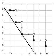
Figure 1. ${\textrm{CFK}}^{\infty}(T(3,7))$

3. Filtrations

We now discuss more general filtrations on vector spaces. In our applications, the vector space will be $\mathrm{CF}(K).$

Definition 3.1.

A real-valued (discrete) filtration on a vector space $\mathrm{C}$ is a collection of subspaces $\mathcal{F}=\{\mathrm{C}_{s}\}$ indexed by the real numbers. This collection must satisfy the following properties:

1. $\mathrm{C}_{s_{1}}\subseteq\mathrm{C}_{s_{2}}$ if $s_{1}\leq s_{2}$.

2. $\mathrm{C}=\cup_{s\in\mathbb{R}}\mathrm{C}_{s}$.

3. $\cap_{s\in\mathbb{R}}\mathrm{C}_{s}=\{0\}$.

4. (discreteness) $\mathrm{C}_{s_{2}}/\mathrm{C}_{s_{1}}$ is finite dimensional when $s_{1}\leq s_{2}$.

Given a discrete filtration $\mathcal{F}=\{\mathrm{C}_{s}\}$ on $\mathrm{C}$, we can define an associated function on $\mathrm{C}$, which we temporarily also denote by $\mathcal{F}$, given by $\mathcal{F}(x)=\min\{s\in\mathbb{R}\ |\ x\in\mathrm{C}_{s}\}$. Notice that $\mathcal{F}^{-1}((-\infty,s])=\mathrm{C}_{s}$.

Given an arbitrary real-valued function $f$ on $\mathrm{C}$, one can define an associated filtration with $\mathrm{C}_{s}=\text{Span}(f^{-1}((-\infty,s]))$. The resulting filtration need not be discrete.

Notation. In cases in which more than one filtration might be under consideration, we will write $(\mathrm{C},\mathcal{F})_{s}$ rather than $\mathrm{C}_{s}$.

Definition 3.2.

A set of vectors $\{z_{i}\}$ in the real filtered vector space $\mathrm{C}$ is called a filtered basis if it is linearly independent and every $\mathrm{C}_{s}$ has some subset of $\{z_{i}\}$ as a basis. If $\mathrm{C}$ is also graded, $\mathrm{C}=\oplus_{i=-\infty}^{\infty}G_{i}$, then we say the basis is a filtered graded basis if each $\mathrm{C}_{s}\cap G_{k}$ has a subset of $\{z_{i}\}$ as a basis.

4. The definition of the filtration $\mathcal{F}_{t}$ on $\mathrm{CF}(K)$.

For any $t\in[0,2]$, the convex combination of Alexander and algebraic filtrations, $\frac{t}{2}Alex+(1-\frac{t}{2})Alg$, defines a real-valued function on $\mathrm{CF}(K)$, to which we associate a filtration denoted $\mathcal{F}_{t}$. That is, for all $s\in\mathbb{R}$, $(\mathrm{CF}(K),\mathcal{F}_{t})_{s}$ is spanned by all vectors $x\in\mathrm{CF}(K)$ such that $\frac{t}{2}Alex(x)+(1-\frac{t}{2})Alg(x)\leq s$.

Theorem 4.1.

If $0\leq t\leq 2$, the filtration $\mathcal{F}_{t}$ on $\mathrm{CF}(K)$ is a filtration by subcomplexes and is discrete. The action of $U$ lowers filtration levels by 1.

Proof.

To see that these are subcomplexes, suppose that $x\in(\mathrm{CF}(K),\mathcal{F}_{t})_{s}$. Write $x=\sum x_{i}$ where $\frac{t}{2}Alex(x_{i})+(1-\frac{t}{2})Alg(x_{i})\leq s$ for all $i$. Since $\partial x=\sum\partial x_{i}$, we only need to check that for each $i$, $\partial x_{i}\in(\mathrm{CF}(K),\mathcal{F}_{t})_{s}$. Let $x_{i}$ have $Alex(x_{i})=a$ and $Alg(x_{i})=b$. Then $Alex(\partial x_{i})=a^{\prime}\leq a$ and $Alg(\partial x_{i})=b^{\prime}\leq b.$ Since both $\frac{t}{2}$ and $(1-\frac{t}{2})$ are nonnegative, $\frac{t}{2}a^{\prime}+(1-\frac{t}{2})b^{\prime}\leq\frac{t}{2}a+(1-\frac{t}{2})b\leq s$, as desired.

The discreteness of the filtration depends on two properties of $\mathrm{CF}(K)$. First, letting $g$ denote the three-genus, $g_{3}(K)$, according to [8] one has $-g\leq Alex(x)-Alg(x)\leq g$ for all $x$. From this it follows that for given $s_{1}<s_{2}$, there are $k_{1}$ and $k_{2}$ in $\mathbb{R}$ such that

$$(\mathrm{CF}(K),Alex)_{k_{1}}\subseteq(\mathrm{CF}(K),\mathcal{F}_{t})_{s_{1}}\subseteq(\mathrm{CF}(K),\mathcal{F}_{t})_{s_{2}}\subseteq(\mathrm{CF}(K),Alex)_{k_{2}}.$$

(The values of $k_{1}$ and $k_{2}$ can be chosen to be $s_{1}-(1-\frac{t}{2})g$ and $s_{2}+(1-\frac{t}{2})g$, respectively, but we do not need this level of detail.) Second, the Alexander filtration is discrete, so the quotient ($\mathrm{CF}(K),Alex)_{k_{2}}/(\mathrm{CF}(K),Alex)_{k_{1}}$ is finite dimensional.

Finally, that $U$ lowers filtration levels by one is immediate. ∎

5. The definition of $\Upsilon_{K}(t)$

For each $t\in[0,2]$ and for all $s\in\mathbb{R}$, the set $(\mathrm{CF}(K),\mathcal{F}_{t})_{s}\subset\mathrm{CF}(K)$ is a subcomplex. Thus, we can make the following definition.

Definition 5.1.

Let $\nu(\mathrm{CF}(K),\mathcal{F}_{t})=\min\{s\ |\ \text{Image\ }(H_{0}((\mathrm{CF}(K),\mathcal{F}_{t})_{s})\to H_{0}(\mathrm{CF}(K))\text{ is surjective}\}$.

Definition 5.2.

$\Upsilon_{K}(t)=-2\nu(\mathrm{CF}(K),\mathcal{F}_{t})$.

5.1. Example

Consider the knot $K=T(3,7)$ with $\mathrm{CF}(K)$ as illustrated in Figure 1. The portion of the complex shown has homology $\mathbb{F}$, at grading 0.

The subcomplex $(\mathrm{CF}(K),\mathcal{F}_{t})_{s}$ is generated by the bifiltered generators with Alexander and algebraic filtration levels satisfying

(5.1) $$Alex\leq\frac{2}{t}s+(1-\frac{2}{t})Alg.$$

Observation The lattice points which contain a filtered generator at filtration level $t$ all lie on a line of slope

$$m=1-\frac{2}{t},$$

with lattice points parametrized by the pair $(Alg,Alex)$. Alternatively, if a line of slope $m$ contains distinct lattice points representing bifiltration levels of generators at the same $\mathcal{F}_{t}$ filtration level, then

$$t=\frac{2}{1-m}.$$

In the diagram for $T(3,7)$ shown in Figure 1, the illustrated line in the plane corresponds to $t=\frac{4}{5}$ and $s=2$. Since the lower half-plane bounded by this line contains a generator of $H_{0}(\mathrm{CF}(K))$, while no half plane bounded by a parallel line with smaller value of $s$ contains such a generator, we have $\Upsilon_{K}(\frac{4}{5})=-2(2)=-4$.

Continuing with $K=T(3,7)$, it is now clear that for $m<-2$ (that is, for $t<\frac{2}{3}$), the least $s$ for which $(\mathrm{CF}(K),\mathcal{F}_{t})_{s}$ contains a generator of $H_{0}(\mathrm{CF}(K))$ corresponds to the line through $(0,6)$, which has filtration level $\frac{t}{2}6+(1-\frac{t}{2})0=3t$.

For $-2<m<-1$ (that is, for $\frac{2}{3}<t<1$), the least $s$ for which $(\mathrm{CF}(K),\mathcal{F}_{t})_{s}$ contains a generator of $H_{0}(\mathrm{CF}(K))$ corresponds to the line through $(2,2)$, which has filtration level $\frac{t}{2}2+(1-\frac{t}{2})2=2$. Multiplying by $-2$ and checking the value $t=\frac{2}{3}$ yields

$$\Upsilon_{T(3,7)}(t)=\begin{cases}-6t&\mbox{if }0\leq t\leq\frac{2}{3}\\ -4&\mbox{if }\frac{2}{3}\leq t\leq 1.\end{cases}$$

6. An alternative definition of $\nu$ and $\Upsilon$

In the appendix we prove Theorem A.1, which has as an immediate consequence the following result.

Theorem 6.1.

The filtered graded chain complex $(\mathrm{CF}(K),\mathcal{F}_{t})$ is isomorphic to a filtered graded complex of the form

$$\mathcal{T}\oplus\mathcal{A},$$

where $\mathcal{T}\oplus\mathcal{A}$ has the structure of a $\Lambda$–module and the isomorphism is a $\Lambda$–module isomorphism. The summand $\mathcal{T}$ has the properties that: (1) it is isomorphic to $\Lambda$ as a $\Lambda$–module; (2) the element $1\in\Lambda\cong\mathcal{T}$ has grading 0. Furthermore, $\mathcal{A}$ is acyclic as an unfiltered complex.

Notice that since all gradings in $\mathcal{T}$ are even, the boundary operator restricted to $\mathcal{T}$ is trivial.

When placed in this simple form, the computation of $\nu((\mathrm{CF}(K),\mathcal{F}_{t}))$ is simple: it is the $\mathcal{F}_{t}$ filtration level of $1\in\Lambda\cong\mathcal{T}$. Hence, we have the following result.

Corollary 6.2.

$\Upsilon_{K}(t)$ equals $-2$ times the $\mathcal{F}_{t}$–filtration level of $1\in\Lambda\cong\mathcal{T}$ for the decomposition $(\mathrm{CF}(K),\mathcal{F}_{t})\cong\mathcal{T}\oplus\mathcal{A}$.

7. Products and additivity

According to [7], there is a (graded) chain homotopy equivelance of complexes

$$\mathrm{CF}(K_{1})\otimes_{\Lambda}\mathrm{CF}(K_{2})\simeq\mathrm{CF}(K_{1}\mathop{\#}K_{2})$$

that preserves the $\Lambda$–structure.

Each of $\mathrm{CF}(K_{1})$, $\mathrm{CF}(K_{2})$ and $\mathrm{CF}(K_{1}\mathop{\#}K_{2})$ has an algebraic filtration. To distinguish these, we write $Alg^{1}$, $Alg^{2}$ and $Alg^{1,2}$. Similarly, the Alexander and $\mathcal{F}_{t}$ filtrations will be distinguish with superscripts.

Momentarily we write $\mathrm{CF}_{1}=\mathrm{CF}(K_{1})$ and $\mathrm{CF}_{2}=\mathrm{CF}(K_{2})$. For each $t\in[0,2]$ the filtrations $\mathcal{F}^{1}_{t}$ and $\mathcal{F}^{2}_{t}$ on $\mathrm{CF}_{1}$ and $\mathrm{CF}_{2}$ induce a filtration $\mathcal{F}_{t}^{1}\otimes\mathcal{F}_{t}^{2}$ on $\mathrm{CF}_{1}\otimes_{\Lambda}\mathrm{CF}_{2}$, defined via:

$$(\mathrm{CF}_{1}\otimes_{\Lambda}\mathrm{CF}_{2},\mathcal{F}_{t}^{1}\otimes\mathcal{F}^{2}_{t})_{s}=\\ \text{Image}(\oplus_{s_{1}+s_{2}=s}\ (\mathrm{CF}_{1},\mathcal{F}^{1}_{t})_{s_{1}}\otimes_{\mathbb{F}}(\mathrm{CF}_{2},\mathcal{F}^{2}_{t})_{s_{2}}\to(\mathrm{CF}_{1},\mathcal{F}^{1}_{t})\otimes_{\Lambda}(\mathrm{CF}_{2},\mathcal{F}_{t}^{2})).$$

Notice that the direct sum is infinite and each summand is infinitely generated. Again, according to [7], for the connected sum of knots, the equivalence

$$\mathrm{CF}(K_{1})\otimes_{\Lambda}\mathrm{CF}(K_{2})\simeq\mathrm{CF}(K_{1}\mathop{\#}K_{2})$$

is a filtered equivalence for both the Alexander and algebraic filtrations. To state this explicitly,

$$(\mathrm{CF}(K_{1}),Alex^{1})\otimes_{\Lambda}(\mathrm{CF}(K_{2}),Alex^{2})\simeq(\mathrm{CF}(K_{1}\mathop{\#}K_{2}),Alex^{1,2})$$

and

$$(\mathrm{CF}(K_{1}),Alg^{1})\otimes_{\Lambda}(\mathrm{CF}(K_{2}),Alg^{2})\simeq(\mathrm{CF}(K_{1}\mathop{\#}K_{2}),Alg^{1,2}).$$

Theorem 7.1.

For all $t\in[0,1]$,

$$(\mathrm{CF}(K_{1}),\mathcal{F}^{1}_{t})\otimes_{\Lambda}(\mathrm{CF}(K_{2}),\mathcal{F}^{2}_{t})\simeq(\mathrm{CF}(K_{1}\mathop{\#}K_{2}),\mathcal{F}^{1,2}_{t}).$$

Proof.

Fix bases $\{x_{i}\}$ and $\{y_{i}\}$ for the free $\Lambda$–modules $\mathrm{CF}(K_{1})$ and $\mathrm{CF}(K_{2})$ so that the sets of all translates $\{U^{k}x_{i}\}$ and $\{U^{k}y_{i}\}$, $k\in\mathbb{Z}$, form graded bifiltered bases for $\mathrm{CF}(K_{1})$ and $\mathrm{CF}(K_{2})$ (as $\mathbb{F}$–vector spaces). The $\mathbb{F}$-vector space $\mathrm{CF}(K_{1})\otimes_{\Lambda}\mathrm{CF}(K_{2})$ is generated by the set of all tensor products, $\{U^{k}x_{i}\otimes U^{j}x_{l}\}$, but note that these do not form a basis; for instance, $Ux\otimes y=x\otimes Uy$.

When selecting elements from $\{U^{k}x_{i}\}$, we will sometimes refer to them as $x$; similarly for $y$. Note that in particular, for such basis elements, $Alg^{1,2}(x\otimes y)=Alg^{1}(x)+Alg^{2}(y)$ and $Alex^{1,2}(x\otimes y)=Alex^{1}(x)+Alex^{2}(y)$.

The proof of the theorem consists of showing that the filtrations $\mathcal{F}^{1}_{t}\otimes\mathcal{F}^{2}_{t}$ and $\mathcal{F}^{1,2}_{t}$ on $\mathrm{CF}(K_{1})\otimes_{\Lambda}\mathrm{CF}(K_{2})$ are the same.

If an element $z\in\mathrm{CF}(K_{1})\otimes_{\Lambda}\mathrm{CF}(K_{2})$ has $\mathcal{F}^{1,2}_{t}$ filtration level $s$, then it can be written as the sum of elements $x\otimes y$ with

$$\frac{t}{2}Alex(x\otimes y)+(1-\frac{t}{2})Alg(x\otimes y)\leq s.$$

This is the same as

$$\frac{t}{2}Alex(x)+(1-\frac{t}{2})Alg(x)+\frac{t}{2}Alex(y)+(1-\frac{t}{2})Alg(y)\leq s.$$

This implies that $\mathcal{F}^{1}_{t}(x)+\mathcal{F}^{2}_{t}(y)\leq s$. This in turn implies that $(\mathcal{F}^{1}_{t}\otimes\mathcal{F}^{2}_{t})(x\otimes y)\leq s$. Thus, for all $z\in\mathrm{CF}(K_{1})\otimes_{\Lambda}\mathrm{CF}(K_{2})$, $(\mathcal{F}^{1}_{t}\otimes\mathcal{F}^{2}_{t})(z)\leq\mathcal{F}^{1,2}_{t}(z)$.

Similarly, suppose that $z\in\mathrm{CF}(K_{1})\otimes_{\Lambda}\mathrm{CF}(K_{2})$ has $\mathcal{F}^{1}_{t}\otimes\mathcal{F}_{t}^{2}$ filtration level $s$. Then it is the sum of elements $x\otimes y$, each of which satisfies $\mathcal{F}_{1}^{t}(x)+\mathcal{F}_{2}^{t}(y)\leq s$. This can be expanded and rewritten as

$$\frac{t}{2}(Alex(x)+Alex(y))+(1-\frac{t}{2})(Alg(x)+Alg(y))\leq s.$$

In other words, $z$ is the sum of elements $x\otimes y$ with $\mathcal{F}^{1,2}_{t}(x\otimes y)\leq s$. Hence, $\mathcal{F}^{1,2}_{t}(x\otimes y)\leq s$. ∎

Theorem 7.1, along with Theorem 6.1, offers a fast proof of the additivity of $\Upsilon$.

Theorem 7.2.

For each $t\in[0,2]$, $\Upsilon_{K_{1}\mathop{\#}K_{2}}(t)=\Upsilon_{K_{1}}(t)+\Upsilon_{K_{2}}(t).$

Proof.

One only needs to check this for complexes of the form $\mathcal{T}\oplus\mathcal{A}$, as given in Theorem 6.1. Acyclic summands do not affect the value of $\Upsilon_{K}(t)$. Thus, we only need consider the case of complexes $\mathcal{T}(K_{1})\otimes_{\Lambda}\mathcal{T}(K_{2})$, for which the statement is clear. ∎

Similarly, Theorem 6.1 offers a fast proof of the following.

Theorem 7.3.

For an arbitrary knot $K$, $\Upsilon_{-K}(t)=-\Upsilon_{K}(t)$.

Proof.

According to [7], the complexes $\mathrm{CF}(K)$ and $\text{CF}(-K)$ are duals: $\text{CF}(-K)\cong\mathrm{CF}(K)^{*}$. More precisely, $\text{CF}(-K)$ is isomorphic to the complex $\text{Hom}_{\mathbb{F}}(\mathrm{CF}(K),\mathbb{F})$, having underlying vector space the space of $\mathbb{F}$–homomorphisms with finite dimensional (that is, finite) support.

If we fix a basis $\{x_{i}\}$ of $\mathrm{CF}(K)$ as a $\Lambda$–module so that the set $\{U^{k}x_{i}\}$ forms a graded bifiltered basis of $\mathrm{CF}(K)$, then we can denote the elements of the dual basis by $(U^{k}x_{i})^{*}$. The dual complex is readily understood in terms of these bases.

1. An easy exercise shows that the action of $U$ on the dual basis is of the form $U(U^{k}x_{i})^{*}=(U^{k-1}x_{i})^{*}$. In particular, the set $\{x_{i}^{*}\}$ forms a basis for the $\Lambda$–module $\mathrm{CF}(K)^{*}$.

2. For any filtration $\mathcal{F}$ on $\mathrm{CF}(K)$, we can define a filtration $\mathcal{F}^{*}$ on the dual space as follows:

   $$(\mathrm{CF}(K)^{*},\mathcal{F}^{*})_{s}=\{\phi\in\mathrm{CF}(K)^{*}\ |\ \phi((\mathrm{CF}(K),\mathcal{F})_{-s^{\prime}})=0\text{ for all }s^{\prime}>s\}.$$

   The choice of signs ensures that the dual filtration is increasing. Thus, $\mathcal{F}^{*}(x_{i}^{*})=-\mathcal{F}(x_{i})$.

3. The boundary operator for the dual space acts in the expected way with respect to basis elements: if $x$ is a component of $\partial y$, then $y^{*}$ is a component of $\partial x^{*}$.

These three observations are easily summarized in terms of diagrams such as in Figure 1: the diagram for $\mathrm{CF}(-K)$ is obtained from that for $\mathrm{CF}(K)$ by rotating the figure by 180 degrees around the origin and reversing all the arrows.

There are two filtrations on $\mathrm{CF}(-K)$ of interest. The first is $\frac{t}{2}Alex^{*}+(1-\frac{t}{2})Alg^{*}$; the second is $\mathcal{F}_{t}^{*}=(\frac{t}{2}Alex+(1-\frac{t}{2})Alg)^{*}$. By using the chosen basis and its dual basis, it is possible to see that these two filtrations are the same, as follows. We use coordinates $(i,j)$ for the plane. For a basis vector $x$, its dual vector $x^{*}$ is in $\mathcal{F}_{t}^{*}$ if and only if it lies on or above the line $\frac{t}{2}j+(1-\frac{t}{2})i=-t$. If this is the case, then when rotated 180 degrees about the origin it lies on or below the line $\frac{t}{2}j+(1-\frac{t}{2})i=t$. These are precisely the dual vectors for which $\frac{t}{2}Alex^{*}+(1-\frac{t}{2})Alg^{*}\leq t$.

The proof of the theorem is now reduced to an elementary calculation for the simple complex $\mathcal{T}(K)$ and its dual $\mathcal{T}(K)^{*}$. ∎

8. Basic properties of $\Upsilon_{K}(t)$ and $\Upsilon^{\prime}_{K}(t)$.

We now present some basic results concerning $\Upsilon_{K}(t)$ and its derivative. An initial observation is that $\Upsilon_{K}(0)=0$ and, since $\mathrm{CF}(K)$ is finitely generated, $\Upsilon_{K}(t)$ is continuous at 0. Thus, we focus on $t>0$.

Theorem 8.1.

1. For every knot $K$, $\Upsilon(K)$ is a continuous piecewise linear function.

2. At a nonsingular point of $\Upsilon^{\prime}_{K}(t)$, the value of $|\Upsilon^{\prime}_{K}(t)|$ is $|i-j|$, where $(i,j)$ is the bifiltration level of some filtered generator of $\mathrm{CF}(K)$ with homological grading 0.

3. Singularities in $\Upsilon^{\prime}_{K}(t)$ can occur only at values of $t$ such that some line of slope $1-\frac{2}{t}$ contains at least two lattice points, $(i,j)$ and $(i^{\prime},j^{\prime})$, each of which represents the algebraic and Alexander gradings of filtered generators of $\mathrm{CF}(K)$ of homological grading $0$.

4. If $\Upsilon^{\prime}_{K}(t)$ has a singularity at $t$, then the jump in $\Upsilon^{\prime}_{K}(t)$ at $t$, denoted $\Delta\Upsilon^{\prime}_{K}(t)$, satisfies $|\Delta\Upsilon^{\prime}_{K}(t)|=\frac{2}{t}|i-i^{\prime}|$ for some pair $(i,i^{\prime})$ for which there are lattice points $(i,j)$ and $(i^{\prime},j^{\prime})$ as in the previous item.

Proof.

The proof is discussed in terms of the diagram of the complex, as illustrated for the knot $T(3,7)$ in the previous section.

Suppose $\Upsilon_{K}(t)=-2s$ and there is precisely one lattice point $(i,j)$ with $\frac{t}{2}j+(1-\frac{t}{2})i=s$ which represents the bifiltration level of a filtered generator of $\mathrm{CF}(K)$. (This will be the case for all but a finite number of values of $t$.) For a nearby $t$, say $t^{\prime}$, the value of $\Upsilon_{K}(t^{\prime})=-2s^{\prime}$ will be such that the same vertex (at $(i,j)$) lies on the line $\frac{t^{\prime}}{2}j+(1-\frac{t^{\prime}}{2})i=s^{\prime}$. That is, for all nearby values of $t$, the value of $s$ is given by $\frac{t}{2}j+(1-\frac{t}{2})i$. Written differently,

$$\Upsilon_{K}(t)=-2i+(i-j)t.$$

In particular, we see that $\Upsilon_{K}(t)$ is piecewise linear off a finite set.

Now consider a singular value of $t$, at which $\Upsilon_{K}(t)=-2s$ and there are two or more pairs $(i,j)$ for which $\frac{t}{2}j+(1-\frac{t}{2})i=s$. Notice that this line in the $(i,j)$–plane has slope $m=1-\frac{2}{t}$. For $t^{\prime}$ close to $t$ and $t^{\prime}<t$, we have

$$\Upsilon_{K}(t^{\prime})=-2i+(i-j)t^{\prime}$$

for one of those pairs $(i,j)$. If $t^{\prime}$ is near $t$ and $t^{\prime}>t$, then

$$\Upsilon_{K}(t^{\prime})=-2i^{\prime}+(i^{\prime}-j^{\prime})t^{\prime}$$

for another (or possibly the same) of these pairs, $(i^{\prime},j^{\prime})$. Notice that these are equal at $t$, giving the continuity of $\Upsilon_{K}(t)$.

We now see that a singularity of $\Upsilon_{K}(t)$ occurs if $(j-i)\neq(j^{\prime}-i^{\prime})$. With these observations, the proofs of (1), (2), and (3) are complete.

For (4), our computations have shown that the change in $\Upsilon^{\prime}_{K}(t)$, denoted $\Delta\Upsilon_{K}^{\prime}(t)$, is given by $\Delta\Upsilon_{K}^{\prime}(t)=(j-j^{\prime})-(i-i^{\prime})$ for some appropriate $(i,j)$ and $(i^{\prime},j^{\prime})$. Since both are assumed to lie on a line of slope $1-\frac{2}{t}$, we have $j-j^{\prime}=(1-\frac{2}{t})(i-i^{\prime})$, so

$$\Delta\Upsilon_{K}^{\prime}(t)=(1-\frac{2}{t})(i-i^{\prime})-(i-i^{\prime})=-\frac{2}{t}(i-i^{\prime}).$$

This completes the proof of the theorem. ∎

Corollary 8.2.

For any knot $K$ and for $t=\frac{p}{q}$ with $\gcd(p,q)=1$,

$$\frac{t}{2}\Delta\Upsilon_{K}^{\prime}(t)=kp,$$

where $k$ is some integer if $p$ is odd, or half-integer if $p$ even.

Proof.

By Theorem 8.1 (4), $|\frac{t}{2}\Delta\Upsilon_{K}^{\prime}(t)|=|i-i^{\prime}|$ for some pair of integers $i$ and $i^{\prime}$, where there are two lattice points on a line of slope $m=1-\frac{2}{t}.$ Thus, we want to constrain the possible differences between the first coordinates of such lattice points.

For $t=\frac{p}{q}$, $m=-\frac{2q-p}{p}$. Since $\gcd(p,q)=1$, in reduced terms, this is either $m=-\frac{2q-p}{p}$ or $m=-\frac{q-(p/2)}{(p/2)}$ if $p$ is odd or even, respectively. Two lattice points on such a line have first coordinates differing by a multiple of $p$ or of $\frac{p}{2}$, if $p$ is odd or even, respectively. The completes the proof. ∎

9. The three-genus, $g_{3}(K)$.

Theorem 9.1.

For nonsingular points of $\Upsilon^{\prime}_{K}(t)$, $|\Upsilon^{\prime}_{K}(t)|\leq g_{3}(K)$.

Proof.

According to [8], if $K$ is of genus $g$, then all elements of $\mathrm{CF}(K)$ have filtration level $(i,j)$, where

$$-g\leq i-j\leq g.$$

It follows immediately from the second statement of Theorem 8.1 that $|\Upsilon_{K}^{\prime}(t)|\leq g_{3}(K)$. ∎

We also observe that the genus of $K$ constrains the possible points of singularity of $\Upsilon^{\prime}_{K}(t)$.

Theorem 9.2.

Suppose that $\Upsilon^{\prime}_{K}(t)$ has a singularity at $t=\frac{p}{q}$, with $\gcd(p,q)=1$. Then:

• If $p$ is odd, $q\leq g_{3}(K)$.

• If $p$ is even, $q\leq 2g_{3}(K)$.

Proof.

Suppose that a line of slope $m=-\frac{a}{b}$, where $0<b<a$ contains two distinct points of the form $(i,j)$ with $|i-j|\leq g_{3}(K)$. It follows quickly that the genus bound implies

$$a\leq 2g_{3}(K)-b.$$

To express this in terms of $t$, suppose $t=\frac{p}{q}$ with $\gcd(p,q)=1$. Then

$$m=1-\frac{2}{t}=-\frac{2q-p}{p}.$$

If $p$ is odd, then $\gcd(2q-p,p)=1$. If $p$ is even, say $p=2k$, then $\gcd(2q-p,p)=\gcd(2q,p)=2$ and $m=-\frac{q-k}{k}$, with $q$ and $k$ relatively prime.

In the first case, with $p$ odd, we have $2q-p\leq 2g_{3}(K)-p$, so $q\leq g_{3}(K)$.

In the second case, with $p$ even, we have $q-k\leq 2g_{3}(K)-k$, so $q\leq 2g_{3}(K)$. ∎

10. $\Upsilon_{K}(t)$ as a knot concordance invariant

If knots $K_{1}$ and $K_{2}$ are concordant, then there is an equality among $d$–invariants: $d(S^{3}_{N}(K_{1}),{{\mathfrak{s}}}_{m})=d(S^{3}_{N}(K_{2}),{{\mathfrak{s}}}_{m})$ for all $N\in\mathbb{Z}$ and $m\in\mathbb{Z}$, $-\frac{N-1}{2}\leq m\leq\frac{N-1}{2}$. Here $S^{3}_{N}(K)$ denotes $N$ surgery on $K$, $d$ is the Heegaard Floer correction term, and ${{\mathfrak{s}}}_{m}$ is a Spin^c structure, with $m$ given by a specific enumeration of Spin^c structures; all are described in [5]. (In the case that $N$ is odd, this range of $m$ includes all possible Spin^c structures.)

If $N$ is large, then $d(S^{3}_{N}(K_{1}),{{\mathfrak{s}}}_{0})=D(K)+S(N)$, where $D(K)$ is the largest grading of a class $z$ in the homology of $\mathrm{CF}(K)_{\{i\leq 0,j\leq 0\}}$ for which $U^{k}z$ is nontrivial for all $k>0$, and $S(N)$ is some rational function defined on the integers, independent of $K$.

In the case that $K$ is slice, we see that the maximal grading $D(K)=D(u)$, where $u$ is the unknot. This implies that for a slice knot $K$, $D(K)=0$. We have a nesting of complexes

$$\mathrm{CF}(K)_{\{i\leq 0,j\leq 0\}}\subset(\mathrm{CF}(K),\mathcal{F}_{t})_{0}.$$

Since $(0,0)$ is at $\mathcal{F}_{t}$ filtration level $0$, it follows that $\nu(\mathrm{CF}(K),\mathcal{F}_{t})\leq 0$; thus $\Upsilon_{K}(t)\geq 0$.

However, $-K$ is also slice, so $-\Upsilon_{K}(t)\geq 0$. It follows that $\Upsilon_{K}(t)=0$. An additive invariant of knots that vanishes on slice knots is a concordance invariant.

11. The concordance-genus

The concordance-genus $g_{c}(K)$ of a knot $K$, defined in [4], is the minimal genus among all knots concordant to $K$. Since $\Upsilon_{K}(t)$ is a concordance invariant, the genus bounds in Section 9 apply to the concordance genus.

Theorem 11.1.

For all nonsingular points of $\Upsilon_{K}(t)$, $|\Upsilon^{\prime}_{K}(t)|\leq g_{c}(K)$. The jumps in $\Upsilon_{K}^{\prime}(t)$ occur at rational numbers $\frac{p}{q}$. For $p$ odd, $q\leq g_{c}(K)$. If $p$ is even, $\frac{q}{2}\leq g_{c}(K)$.

12. Bounds on the four-genus, $g_{4}(K)$.

Let $\mathrm{CF}(K)_{0,m}$ denote the bifiltered subcomplex $\mathrm{CF}(K)_{\{i\leq 0,j\leq m\}}$. We let $\nu^{-}(K)$ denote the minimum value of $m$ such that the homology of $\mathrm{CF}(K)_{0,m}$ contains a nontrivial grading 0 element of the homology of $\mathrm{CF}(K)$, which we recall is isomorphic to $\Lambda$ with 1 at grading 0. There is the following result of Hom and Wu [1], built from work of Rasmussen [10]. (In [1] the invariant $\nu^{+}$ is described; the equivalence with $\nu^{-}$ is presented in [9].)

Proposition 12.1 (Proposition 2.4, [1]).

$\nu^{-}\leq g_{4}(K)$.

Based on this, we show that $\Upsilon_{K}(t)$ provides a bound on $g_{4}(K)$.

Theorem 12.2.

For all $t\in[0,2]$, ${|\Upsilon_{K}(t)|}\leq tg_{4}(K)$.

Proof.

Since $(0,m)$ is at $\mathcal{F}_{t}$ filtration level $tm/2$, we have the containment

$$\mathrm{CF}(K)_{0,m}\subset(\mathrm{CF}(K),\mathcal{F}_{t})_{tm/2}.$$

Since $\mathrm{CF}(K)_{0,\nu^{-}}$ contains an element of grading 0 in the homology of $\mathrm{CF}(K)$, so does the subcomplex $(\mathrm{CF}(K),\mathcal{F}_{t})_{t\nu^{-}/2}$. Thus, $\nu(\mathrm{CF}(K),\mathcal{F}_{t})\leq t\nu^{-}/2$. By the previous proposition, $\nu(\mathrm{CF}(K),\mathcal{F}_{t})\leq tg_{4}(K)/2$.

Considering $-K$, we have $\nu(\mathrm{CF}(-K),\mathcal{F}_{t})\leq tg_{4}(-K)/2$; it follows that $-\nu(\mathrm{CF}(K),\mathcal{F}_{t})\leq tg_{4}(K)/2$. Combining these yields

$$|\nu(\mathrm{CF}(K),\mathcal{F}_{t})|\leq tg_{4}(K)/2.$$

Multiplying by $-2$ yields the desired conclusion. ∎

13. Crossing change bounds

Here we sketch a proof of Proposition 1.10 of [9]. The argument is essentially the same as used in [3] to prove the corresponding fact about $\tau(K)$.

Theorem 13.1.

Let $K_{-}$ and $K_{+}$ be knots with identical diagrams, except at one crossing which is either negative or positive, respectively. Then for $t\in[0,1]$,

$$\Upsilon_{K_{+}}(t)\leq\Upsilon_{K_{-}}(t)\leq\Upsilon_{K_{+}}(t)+t.$$

Proof.

First note that $K_{-}\mathop{\#}-K_{+}$ can be changed into the slice knot $K_{+}\mathop{\#}-K_{+}$ by changing a negative crossing to positive. Thus, $g_{4}(K_{-}\mathop{\#}-K_{+})\leq 1$. It follows that

(13.1) $$-t\leq\Upsilon_{K_{-}}(t)-\Upsilon_{K_{+}}(t)\leq t.$$

Next, note that $K_{-}\mathop{\#}-K_{+}\mathop{\#}\ T(2,3)$ can be changed into the slice knot $K_{+}\mathop{\#}-K_{+}$ by changing one negative crossing to positive and one positive crossing to negative. Thus, it too has four-genus at most 1: it bounds a singular disk with two singularities of opposite sign, and these can be tubed together. A simple computation for $T(2,3)$ yields $\Upsilon_{T(2,3)}(t)=-t$ for $0\leq t\leq 1$. Thus,

$$-t\leq\Upsilon_{K_{-}}(t)-\Upsilon_{K_{+}}(t)-t\leq t,$$

which we rewrite as

(13.2) $$0\leq\Upsilon_{K_{-}}(t)-\Upsilon_{K_{+}}(t)\leq 2t.$$

Combining Equations 13.1 and 13.2,

$$0\leq\Upsilon_{K_{-}}(t)-\Upsilon_{K_{+}}(t)\leq t.$$

Adding $\Upsilon_{K_{+}}(t)$ to all terms yields the desired conclusion,

$$\Upsilon_{K_{+}}(t)\leq\Upsilon_{K_{-}}(t)\leq\Upsilon_{K_{+}}(t)+t.$$

∎

Note This argument can be easily modified to show that if there is a singular concordance from $K$ to $J$ with a single positive double point, then $\Upsilon_{K}(t)\leq\Upsilon_{J}(t)\leq\Upsilon_{K}(t)+t.$

14. The Ozsváth-Szabó $\tau$-invariant and $\Upsilon_{K}(t)$ for small $t$

For small $t$, $\Upsilon_{K}(t)$ is determined by the $\tau$ invariant defined in [6]. We review the definition below. Here is the statement of the result.

Theorem 14.1.

For $t$ small, $\Upsilon_{K}(t)=-\tau(K)t$.

The subquotient complex $\mathrm{CF}(K)_{\{i\leq 0\}}/\mathrm{CF}(K)_{\{i<0\}}$ will be denoted $\widehat{\mathrm{CF}}(K)$. (Usually, $\widehat{\mathrm{CF}}$ is written $\widehat{{\textrm{CFK}}}$.) It is filtered by the Alexander filtration and has homology $\mathbb{F}$, supported in grading 0. The invariant $\tau(K)$ is defined to be the least integer $\tau$ such that the map on homology $H_{0}(\widehat{\mathrm{CF}}(K)_{\{j\leq\tau\}})\to H_{0}(\widehat{\mathrm{CF}}(K))\cong\mathbb{F}$ is surjective.

We wish to relate $\tau(K)=\tau$ to an invariant of $\mathrm{CF}(K)$. The needed technical result is the following.

Lemma 14.2.

If $\tau(K)=\tau$, then there is a cycle $w\in\mathrm{CF}(K)_{\{i\leq 0,j\leq\tau\}\cup\{i<0\}}$ representing a nontrivial element in $H_{0}(\mathrm{CF}(K))$.

Proof.

From the definition of $\tau$ we see that there is a chain $x\in\mathrm{CF}(K)_{\{i\leq 0,j\leq\tau\}\cup\{i<0\}}$ that in the quotient $\widehat{\mathrm{CF}}(K)$ is a cycle that represents a generator of $H_{0}(\widehat{\mathrm{CF}}(K))$.

Since the chain $x$ represents a cycle in $\widehat{\mathrm{CF}}(K)$, it has the property that $\partial x=y$, where $y\in\mathrm{CF}(K)_{i<0}$. Note that $y$ is a cycle and $gr(y)=-1$. Since $H_{-1}(\mathrm{CF}(K)_{i<0})=0$, there is a chain $z\in\mathrm{CF}(K)_{i<0}$ with $\partial z=y$. Thus, $x+z$ is a cycle in $\mathrm{CF}(K)_{\{i\leq 0,j\leq\tau\}\cup\{i<0\}}$. The map $H_{0}(\mathrm{CF}(K)_{i\leq 0})\to H_{0}(\widehat{\mathrm{CF}}(K))$ is an isomorphism; both groups are isomorphic to $\mathbb{F}$. Thus, $x+z$ represents a generator of $H_{0}(\mathrm{CF}(K)_{i\leq 0}$). The map $H_{0}(\mathrm{CF}(K)_{i\leq 0})\to H_{0}(\mathrm{CF}(K))$ is an isomorphism, completing the proof. ∎

Proof, Theorem 14.1.

For $t$ small, we consider the filtration $\mathcal{F}_{t}$ and the filtration level $s=\frac{t}{2}\tau$. Then one has $\mathrm{CF}(K)_{s}=\mathrm{CF}(K)_{\{i\leq 0,j\leq\tau\}\cup\{i<0\}}$. By Lemma 14.2, this subcomplex contains a cycle that represents an element of grading 0 in $H(\mathrm{CF}(K))$. Thus, for this $\mathcal{F}_{t}$ filtration, $\nu\leq\frac{t}{2}\tau$.

On the other hand, suppose that $\nu<\frac{t}{2}\tau$. Then there would exist a cycle

$$z\in\mathrm{CF}(K)_{\{i\leq 0,j\leq\tau-1\}\cup\{i<0\}}$$

representing a generator of $H(\mathrm{CF}(K))$ of grading 0. However, the image of $z$ in $\widehat{\mathrm{CF}}(K)$ would be an element in $\widehat{\mathrm{CF}}(K)_{\tau-1}$ that represents a generator of $H_{0}(\widehat{\mathrm{CF}}(K))$. But $\tau$ is by definition the lowest level at which this can occur. Thus, we see that $\nu=\frac{t}{2}\tau$.

To conclude, recall that $\Upsilon_{K}(t)=-2\nu$, so $\Upsilon_{K}(t)=-\tau(K)t$, as desired. ∎

Note. With care, one can check that in this argument, the condition that $t$ be small can be made precise by requiring that $t<1/g_{3}(K)$. Of course, once the result is established for some set of small $t$, then Theorem 9.2 provides the bound $t<1/g_{3}(K)$.

15. Equivalence of definitions of $\Upsilon_{K}(t)$

In this section we explain why $\Upsilon_{K}(t)$ as defined here agrees with that of [9].

Beginning with $\mathrm{CF}(K)$, a new complex $t\mathrm{CF}(K)$ can be constructed as follows. As an $\mathbb{F}$–vector space,

$$t\mathrm{CF}(K)=\mathrm{CF}(K)\otimes_{\Lambda}\mathbb{F}[v^{1/n},v^{-1/n}],$$

where $U$ acts on $\mathbb{F}[v^{1/n}]$ via multiplication by $v^{2}$. This has the structure of an $\mathbb{F}[v^{1/n},v^{-1/n}]$–module. To simplify notation, we write $\Lambda^{\prime}=\mathbb{F}[v^{1/n},v^{-1/n}]$.

There are (rational) filtrations $Alg$ and $Alex$ on $t\mathrm{CF}(K)$ which are consistent with those on the $\Lambda$–submodule $\mathrm{CF}(K)$. The action of $v^{1/n}$ lowers filtration levels by ${1}/{2n}$. Thus, $U=v^{2}$ lowers filtration levels by 1, as it should. Similarly, the Maslov grading $M(x)$ naturally extends to $t\mathrm{CF}(K)$ so that the action of $v^{1/n}$ lowers this grading by $1/n$, and thus $U=v^{2}$ continues to lower the Maslov grading by 2.

There is a rational grading on $t\mathrm{CF}(K)$ defined via the Maslov grading, $M$, along with the algebraic and Alexander filtrations. If $x$ is an element at filtration level $(i,j)$, then:

(15.1) $$\text{gr}_{t}(x)=M(x)-t(j-i).$$

(In [9], only generators at algebraic filtration level 0 are used to define gr_t, so $i=0$ and the formula $\text{gr}_{t}(x)=M(x)-tAlex(x)$ is presented.) One checks that $U$ to lowers $\text{gr}_{t}$–gradings by 2, so on the extension to $t\mathrm{CF}(K)$, $v$ lowers gradings by $1$ and $v^{1/n}$ lowers gradings by $1/n$.

If $x$ is a filtered generator of $\mathrm{CF}(K)$ with $\partial x=\sum y_{l}$, then the boundary $\partial_{t}$ is defined so that $\partial_{t}x=\sum v^{\alpha_{l}}y_{l}\in t\mathrm{CF}(K)$, with the values of $\alpha_{l}$ given explicitly in [9]. This extends naturally to a boundary operator on all of $t\mathrm{CF}(K)$.

Given that the operator $\partial_{t}$ is well-defined, it is a simple matter to determine its value. Suppose that $x$ is a filtered generator of $\mathrm{CF}(K)$ at filtration level $(i,j)$, Maslov grading $g$, and suppose also that $\partial x=\sum y_{l}$. Let $y$ denote one of the terms in this sum, at filtration level $(i^{\prime},j^{\prime})$, necessarily of grading $g-1$. Then viewed as an element of $t\mathrm{CF}$, $x$ is of grading $g-t(j-i)$, and $y$ has grading $g-1-t(j^{\prime}-i^{\prime})$. In $\partial_{t}x$, the term $v^{\alpha}y$ appears, and $\alpha$ is such that gr.${}_{t}(v^{\alpha}y)=\text{gr}_{t}(x)-1$. Rewriting this, we have $(g-1)-t(j^{\prime}-i^{\prime})-\alpha=g-t(j-i)-1$. That is,

(15.2) $$\alpha=t((j-j^{\prime})-(i-i^{\prime})).$$

As two examples, Figure 2 illustrates the complexes $t\mathrm{CF}(K)$ for $K=T(3,7)$, with $t=\frac{1}{3}$ and $t=2$. The construction is straightforward using Equation 15.1 and the fact that $v$ shifts along the diagonal a distance of $1/2$ down and to the left. The portion of the complex illustrated was chosen because its homology is $\mathbb{F}$ in grading 0 and represents the generator of the homology of $t\mathrm{CF}$ in grading 0. In the case that $t=\frac{1}{3}$, the full complex consists of the illustrated complex along with all its translates a distance $\frac{k}{6}$, $k\in\mathbb{Z}$, along the diagonal. In the case of $t=2$, the translates are those a distance $\frac{k}{2}$ along the diagonal.

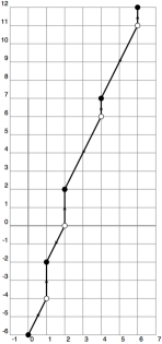
Figure 2. $t\mathrm{CF}_{t=1/3}(T(3,7))$ and $t\mathrm{CF}_{t=2}(T(3,7))$

It is apparent from these examples that the Alexander filtration is not a filtration of the chain complex, since some arrows increase the Alexander filtration level. However, as is easily verified, the algebraic filtration is a filtration on the chain complex.

Definition 15.1.

For $t=\frac{m}{n}$, denote by $t{\textrm{CFK}}^{-}(K)$ the complex $t\mathrm{CF}(K)_{{i\leq 0}}$.

Note. In [9], this complex is denoted $t{\textrm{CFK}}(K)$. In fact, it is the complex that is explicitly constructed. Here we first introduced the infinity complex to be consistent with our earlier constructions.

Definition 15.2.

For $t=\frac{m}{n}$, $\Upsilon_{K}(t)$ is the maximal grading of a class in the homology of $t{\textrm{CFK}}^{-}(K)$ that maps to a nontrivial element in the homology of $t\mathrm{CF}(K)$. Equivalently, it is the maximal grading of a class in the homology of $t{\textrm{CFK}}^{-}(K)$ which is not in the kernel of $v^{k}$ for all $k>0$.

Lemma 15.3.

The value of $\Upsilon_{K}(t)$ as just defined is equal to $-2s$, where $s$ is the least number for which the homology of $t\mathrm{CF}(K)_{i\leq s}$ contains an element of grading 0 that represents a nontrivial element of the homology of $t\mathrm{CF}(K)$.

Proof.

This follows from a simple change of coordinates. ∎

15.1. The two definitions of $\Upsilon_{K}(t)$ agree.

Suppose that using this definition of $\Upsilon_{K}(t)$, we have $\Upsilon_{K}(t)=-2s$. This implies that $t\mathrm{CF}(K)_{i\leq s}$ contains a cycle $z$ representing a nontrivial generator of grading 0 in the homology of $t\mathrm{CF}(K)$. Write $z=\sum x_{l}$, where the $x_{l}$ are filtered generators. Some $x_{l}$ has filtration level $(s,j)$, and none of the $x_{l}$ has algebraic filtration level greater than $s$.

From the regrading formula given in Equation 15.1, $\text{gr}_{t}(x)=M(x)-t(j-i)$, we see that generators of $\mathrm{CF}(K)$ at filtration level $(i,j)$ and grading 0 yield generators of grading 0 in $t\mathrm{CF}(K)$ at filtration level $(i+\frac{t}{2}(j-i),j+\frac{t}{2}(j-i))$. (Recall that shifting down and to the left by $t$ units decreases the grading by $2t$.) We are thus led to consider the transformation

$$(i,j)\mapsto((1-\frac{t}{2})i+\frac{t}{2}j,-\frac{t}{2}i+(1+\frac{t}{2})j).$$

Its inverse is given by

$$(i,j)\mapsto((1+\frac{t}{2})i-\frac{t}{2}j,\frac{t}{2}i+(1-\frac{t}{2})j).$$

Under this transformation, for a fixed value of $s$, the vertical line $\{(s,z)\ |\ z\in{\mathbb{R}}\}$, is carried to the line (in the $\mathrm{CF}(K)$–plane) $\{((1+\frac{t}{2})s-\frac{t}{2}z,\frac{t}{2}s+(1-\frac{t}{2})z)\ |\ z\in{\mathbb{R}}\}.$ Relabeling the coordinate system $(x,y)$, this is the line

$$y=(1-\frac{2}{t})x+(\frac{2}{t})s.$$

Comparing with Equation 5.1, we see that the homology of the filtered complex $(\mathrm{CF}(K),\mathcal{F}_{t})_{s}$ contains a generator of grading 0 that is nontrivial in the homology of $\mathrm{CF}(K)$, and that this is not the case for $(\mathrm{CF}(K),\mathcal{F}_{t})_{s^{\prime}}$ for any $s^{\prime}<s$. Thus, the value of $\Upsilon_{K}(t)$ as defined in Section 5 is $-2s$, and the definitions agree.

Appendix A A structure theorem for $\mathrm{CF}(K)$.

In [2, Chapter 11], vertical and horizontal reductions of $\mathrm{CF}(K)$ are discussed. That presentation applies to the filtered complex $(\mathrm{CF}(K),\mathcal{F}_{t})$, but adjustments in the details would be required because, for instance, the horizontal and vertical filtrations are integer valued rather than being real filtrations. Since the argument in the present case is straightforward, we present it in detail.

Viewed as a $\Lambda$–module, $\mathrm{CF}(K)$ is freely generated by a finite set $\{w_{i}\}_{1\leq i\leq m}$. We again simplify notation by suppressing the indexing set and write $\{w_{i}\}$. This set can be chosen so that the set $\{U^{k}w_{i}\}_{k\in\mathbb{Z}}$ forms a bifiltered graded basis for the $\mathbb{F}$–complex $\mathrm{CF}(K)$. We will refer to any such set $\{w_{i}\}$ as a $\Lambda$–basis for $\mathrm{CF}(K)$. A $\Lambda$–module change of basis among the $w_{i}$ that preserves gradings and filtration levels induces a change of bifiltered graded basis for the $\mathbb{F}$–complex $\mathrm{CF}(K)$. We will refer to any such change of basis as a $\Lambda$–change of basis of $\mathrm{CF}(K)$. Analogous notation will be used when working with the filtered graded complex $(\mathrm{CF}(K),\mathcal{F}_{t})$.

Theorem A.1.

Let $t\in[0,2]$. As a $\Lambda$–module, $\mathrm{CF}(K)$ has a basis $\{\alpha,\beta_{1},\ldots,\beta_{k}\}$, inducing a splitting of $\mathrm{CF}(K)$ (as a $\Lambda$–module) as the direct sum $\mathrm{CF}(K)\cong\mathcal{T}\oplus\mathcal{A}$, where $\mathcal{T}$ is freely generated by $\alpha$ and $\mathcal{A}$ is freely generated by $\{\beta_{1},\ldots,\beta_{k}\}$. This splitting has the following properties.

• $(\mathrm{CF}(K),\mathcal{F}_{t})\cong\mathcal{T}\oplus\mathcal{A}$ as a filtered graded $\mathbb{F}$-complex.

• The complex $\mathcal{T}$ has filtered graded basis $\{U^{k}\alpha\}_{k\in\mathbb{Z}}$, the boundary map is trivial on $\mathcal{T}$, and $gr(\alpha)=0$.

• The complex $\mathcal{A}$ has filtered graded basis $\{U^{k}\alpha_{i}\}_{k\in\mathbb{Z}}$ and has trivial homology: $H(\mathcal{A})=0$.

Proof.

We begin with the $\Lambda$–generating set of $\mathrm{CF}(K)$, $\{w_{i}\}$. By replacing generators with their $U^{k}$ translates and renaming the generators, we can decompose this into two subsets: $\{x_{i}\}$, all of grading 0, and $\{y_{i}\}$, all of grading $1$.

To simplify notation, we abbreviate the filtered graded $\mathbb{F}$–complex $(\mathrm{CF}(K),\mathcal{F}_{t})$ by $\mathrm{CF}_{t}$.

1. Let $A$ be a cycle in $\mathrm{CF}_{t}$ having the least filtration level among cycles representing nontrivial classes in $H_{0}(\mathrm{CF}_{t}).$ After reordering the generators, we can write $A=x_{1}+\cdots+x_{k}$, with the filtration levels nonincreasing. Replacing $x_{1}$ with $x_{1}+\cdots+x_{k}$ as the first generating element (over $\Lambda$) induces a filtered change of basis for $\mathrm{CF}_{t}$. Thus, the first element of the $\Lambda$–basis, which we now denote $A_{1}$, is a cycle of least filtration level representing a nontrivial element of $H_{0}(\mathrm{CF}_{t})$.

2. Consider the set of all generating elements $y_{i}$ that have the property that $A_{1}$ is a component of $\partial y_{i}$. After reordering the basis, we can assume these are $\{y_{1},y_{2},\ldots,y_{k}\}$ for some $k$, and that the filtrations are in nondecreasing order. Make the $\Lambda$–change of basis that replaces each $y_{i}$, $2\leq i\leq k$, with $y_{i}+y_{1}$. This induces a filtered change of basis of $\mathrm{CF}_{t}$. Now, the only generator having $A_{1}$ as a component of its boundary is $y_{1}$, which we relabel $B_{1}$.

3. After perhaps reordering the $x_{i}$, we have either $\partial B_{1}=A_{1}$ or $\partial B_{1}=A_{1}+x_{2}+\cdots+x_{k}$ for some $k\geq 2$, with the filtration levels nonincreasing. Since $\partial^{2}=0$, it follows that $B_{1}$ is not a component of any element in the image of $\partial$.

   If $\partial B_{1}=A_{1}$, then we see that $\{A_{1},B_{1}\}$ generates an acyclic summand of $\mathrm{CF}_{t}$, and thus $A_{1}$ would not represent a nontrivial element in homology.

   We have $\partial B_{1}=A_{1}+x_{2}+\cdots x_{k}$ for some $k\geq 2$. Make the $\Lambda$–change of basis that replaces $x_{2}$ with $x_{2}+\cdots x_{k}$, now calling this new element $A_{2}$. Then $\partial B_{1}=A_{1}+A_{2}$. Note that since $A_{1}$ is a cycle and $A_{1}+A_{2}=\partial B_{1}$ is a cycle, that $A_{2}$ is a cycle representing the same homology class as $A_{1}$. Hence the filtration level of $A_{2}$ is greater than or equal to that of $A_{1}$.

4. We now repeat the previous argument, making a change of basis so that the only basis elements with boundary that include $A_{2}$ as a component are $B_{1}$ and perhaps a second generator that we denote $B_{2}$.

5. This step-by-step procedure must eventually stop, at which time there is constructed a summand of the $\mathbb{F}$–complex $\mathrm{CF}_{t}$

   $$D=A_{1}\leftarrow B_{1}\rightarrow A_{2}\leftarrow B_{2}\rightarrow A_{3}\leftarrow\cdots\rightarrow B_{k-1}\rightarrow A_{k}.$$

   Note that the process must end with an $A_{k}$; if it stopped with a $B_{k}$, the resulting complex would be acyclic and thus not contain a nontrivial element in homology. This complex is a summand of the complex $\mathrm{CF}_{t}$. Note that $\Lambda D$ is a summand of a direct sum decomposition of $\mathrm{CF}_{t}$, as a subcomplex and also as a submodule of the $\Lambda$–module.

6. Since $A_{1}$ has the lowest filtration level among the $A_{i}$, we can replace each $A_{i}$ with $A_{1}+A_{i}$ to form a new basis. The complex then splits in the following way:

   $$A_{1}\ \ \oplus\ \ \left[B_{1}\rightarrow(A_{1}+A_{2})\leftarrow B_{2}\rightarrow(A_{1}+A_{3})\leftarrow\cdots\rightarrow B_{k-1}\rightarrow(A_{1}+A_{k})\right].$$

   We let $\mathcal{T}=\Lambda A_{1}$. It satisfies the required conditions of the theorem. Since as a $\Lambda$–module, $H(\mathcal{T})\cong H(\mathrm{CF}_{t})$, the complementary summand to $\mathcal{T}$ must be acyclic. That complementary summand yields the summand $\mathcal{A}$ in the statement of the theorem.

∎

References

- [1] J. Hom and Z. Wu, Four-ball genus bounds and a refinement of the Ozsváth-Szabó tau-invariant, arxiv.org/abs/1401.1565.
- [2] R. Lipshitz, P. Ozsváth, and D. Thurston, Bordered Heegaard Floer homology, arxiv.org/abs/0810.0687.
- [3] C. Livingston, Computations of the Ozsváth-Szabó knot concordance invariant, Geom. Topol. 8 (2004), 735–742.
- [4] C. Livingston, The concordance genus of knots, Alg. and Geom. Top. 4 (2004), 1–22.
- [5] P. Ozsváth and Z. Szabó, Absolutely graded Floer homologies and intersection forms for four-manifolds with boundary, Adv. Math. 173 (2003), 179–261.
- [6] P. Ozsváth and Z. Szabó, Knot Floer homology and the four-ball genus, Geom. Topol. 7 (2003), 615–639.
- [7] P. Ozsváth and Z. Szabó, Holomorphic disks and knot invariants, Adv. Math. 186 (2004), 58–116.
- [8] P. Ozsváth and Z. Szabó, Holomorphic disks and genus bounds, Geom. Topol. 8 (2004), 311–334.
- [9] P. Ozsváth, A. Stipsicz, and Z. Szabó, Concordance homomorphisms from knot Floer homology, arxiv.org/abs/1407.1795.
- [10] J. Rasmussen, Floer homology and knot complements, arxiv.org/abs/math/0306378.