Relevance of instantons in Burgers turbulence

Abstract

Instanton calculations are performed in the context of stationary Burgers turbulence to estimate the tails of the probability density function (PDF) of velocity gradients. These results are then compared to those obtained from massive direct numerical simulations (DNS) of the randomly forced Burgers equation. The instanton predictions are shown to agree with the DNS in a wide range of regimes, including those that are far from the limiting cases previously considered in the literature. These results settle the controversy of the relevance of the instanton approach for the prediction of the velocity gradient PDF tail exponents. They also demonstrate the usefulness of the instanton formalism in Burgers turbulence, and suggest that this approach may be applicable in other contexts, such as 2D and 3D turbulence in compressible and incompressible flows.

The stochastically driven Burgers equation reads burgers:1974

$$u_{t}+uu_{x}-\nu u_{xx}=\eta,$$ (1)

where $\eta$ is a white-noise forcing satisfying

$$\langle\eta(x,t)\eta(x^{\prime},t^{\prime})\rangle=\delta(t-t^{\prime})\chi(x-x^{\prime}),$$ (2)

in which the spatial correlation $\chi(x)$ has characteristic length $L$ and amplitude $\chi(0)=\chi_{0}$. Besides having a wide range of applications e.g. in the context of structure formation in the early universe arnold-zeldovich-etal:1982 ; shandarin-zeldovich:1989 , traffic flow chowdhury-santen-etal:2000 , growth processes kardar-parisi-etal:1986 , etc. (see e.g. bec-khanin:2007 for an overview), this equation has also gained considerable interest as a toy-model to benchmark techniques for analyzing turbulence. This is due mainly to the phenomenological simplicity of the solutions to (1): In stationary Burgers turbulence, velocity perturbations with negative gradient evolve into shocks, while positive gradients are smoothed out. The shocks have a dramatic influence on the statistics of the velocity field: for example, they are responsible for the anomalous scaling of the velocity increments and they make the probability density function (PDF) of the velocity gradient highly non-Gaussian. These features are signatures of intermittency, the understanding of which has been the main issue in turbulence theory frisch:1995 .

In the context of Burgers turbulence, both the scaling of the right tail of the velocity gradient PDF polyakov:1995 ; gurarie-migdal:1996 ; e-khanin-etal:1997 ; gotoh-kraichnan:1998 and that of its left tail in the inviscid case e-vandeneijnden:2000 ; gotoh-kraichnan:1998 ; boldyrev-linde-polyakov:2004 are known. In contrast, the scaling of the left tail in the viscid case gotoh:1999 ; balkovsky-falkovich-etal:1997 remains more controversial: In particular there is an inconsistency between measurements of the exponent of the tail decay in direct numerical simulations (DNS) gotoh:1999 and the predictions made in balkovsky-falkovich-etal:1997 . The latter were obtained through approximations within the framework of the instanton method gurarie-migdal:1996 ; falkovich-kolokolov-etal:1996 ; balkovsky-falkovich-etal:1997 , which is a field-theoretic approach that has been used in hydrodynamic turbulence. Due to its non-perturbative nature the instanton method is in principle well-suited to study the probability and evolution of rare and extreme events (i.e. the most singular/dissipative structures of the flow) that are responsible for intermittency. This possibilty was also confirmed recently by the numerical computation chernykh-stepanov:2001 ; grafke-grauer-schaefer-vandeneijnden:2014 and successful observation of instantons in actual Burgers turbulence grafke-grauer-schaefer:2013 . The main aim of the present paper is to investigate further the range of applicability of the instanton method in this setup. In particular, we revisit the results of balkovsky-falkovich-etal:1997 , where approximations were made that permit to solve the instanton equations asymptotically and predict that the left tail of the PDF is captured by a compressed exponential with a given exponent. We show that these results are backed up by numerical solutions to the instanton equations, but only apply in the very far tail. Away from this tail, the approximations made in balkovsky-falkovich-etal:1997 fail and numerical solution of the exact instanton equations shows that the PDF is no longer a compressed exponential. These predictions are in agreement with measurements from DNS over a wide range of gradients. This explains why the DNS results in gotoh:1999 , which were believed to contradict the instanton predictions, are in fact consistent with this approach.

We begin by nondimensionalizing (1). If we measure length in units of $L$, time in units of $L^{2}/\nu$, and (consistently) velocity in units of $\nu/L$, (1) becomes

$$u_{t}+uu_{x}-u_{xx}=\sigma\eta$$ (3)

where $\eta$ satisfies (2) with $\chi(x)$ having now characteristic length 1 and amplitude $\chi(0)=1$, and we defined

$$\sigma=\chi^{1/2}_{0}L^{2}\nu^{-3/2}\,.$$ (4)

Up to boundary effects whose impact can be made negligible by making the system size bigger, this parameter is the only control parameter left in the system. It can be related to the Reynolds number $\text{Re}=UL/\nu$ as $\sigma=\text{Re}^{3/2}$ if we use as characteristic velocity $U=(\chi_{0}L)^{1/3}$ – this velocity is the root-mean-square velocity in the turbulent regime when the dissipation scale $L_{d}=\nu^{3/4}\chi_{0}^{-1/4}$ is much smaller than $L$ (i.e. Re and $\sigma$ are much bigger than 1) and an inertial range develops.

The instanton method that we will use to analyze (3) relies on Martin-Siggia-Rose/Janssen/de Dominicis formalism martin-siggia-rose:1973 ; dedominicis:1976 ; janssen:1976 . The saddle point or instanton approximation can be made rigorous within the framework of large deviation theory varadhan:2008 . Within this formalism the expectation of any observable $\mathcal{O}[u]$ of the velocity field $u$ is represented as the path integral

$$\langle\mathcal{O}[u]\rangle\propto\int Du\,\int D(ip)\mathcal{O}[u]\exp(-\sigma^{-2}I[u,p])$$ (5)

where $\langle\cdot\rangle$ denotes expectation with respect to the invariant measure of (1) and

$$I[u,p]=\int_{-\infty}^{0}\left(\langle p,\dot{u}+uu_{x}-u_{xx}\rangle-\tfrac{1}{2}\langle p,\chi\star p\rangle\right)dt$$ (6)

is the action functional for (1). Here, $\langle\cdot,\cdot\rangle$ is the $L_{2}(\mathbb{R})$-scalar product and $\star$ denotes convolution. Since we are interested in strong velocity gradients, we set

$$\mathcal{O}[u]=\exp(\sigma^{-2}\lambda u_{x}(0,0))$$ (7)

Indeed, if $S_{*}(\lambda)=\sigma^{2}\ln\langle e^{\sigma^{-2}\lambda u_{x}(0,0)}\rangle$ and $p(a)$ denotes the PDF of $u_{x}(0,0)=a$, for large $\sigma^{-2}|\lambda|$ we have

$$S_{*}(\lambda)\equiv\sigma^{2}\ln\int_{\mathbb{R}}e^{\sigma^{-2}\lambda a}p(a)da\sim\max_{a}(\lambda a-S(a))$$ (8)

where $S(a)=-\sigma^{2}\ln p(a)$ and we used Laplace’s method to estimate the integral. This means that $S_{*}(\lambda)$ is the Fenchel-Legendre transform of $S(a)$, which also implies that

$$S(a)\sim\max_{\lambda}(\lambda a-S_{*}(\lambda))$$ (9)

For large $\sigma^{-2}|\lambda|$ we can also relate $S_{*}(\lambda)$ and $S(a)$ to the saddle point of the path integral in (5) for the observable in (7), i.e. to the minimizer of the action $I[u,p]-\lambda u_{x}(0,0)$. Specifically

$$I[u^{*},p^{*}]=\lambda u_{x}^{*}(0,0)-S_{*}(\lambda)\sim S(u_{x}^{*}(0,0))$$ (10)

where $(u^{*},p^{*})$ denote the minimizer, termed the instanton, i.e. the solution to

$$u_{t}+uu_{x}-u_{xx} =\chi\star p$$ (11)

$$p_{t}+up_{x}+p_{xx} =0$$

with boundary conditions

$$u(t=-\infty)=0,\qquad p(t=0)=-\lambda\delta^{\prime}(x).$$ (12)

The final condition for $p$ arises from incorporating the term $-\lambda u_{x}(0,0)$ in the variational problem. By varying $\lambda$, we can access different values of the gradient, $u_{x}^{*}(0,0)$ and then use (10) to compute $S(u_{x}^{*}(0,0))$. Carrying on this program therefore allows us to estimate $S(a)$ for different values of $a$. Note that this function is independent of the control parameter $\sigma$ (and hence the Reynolds number $\text{Re}=\sigma^{3/2}$) since we have scaled this parameter out the instanton equations (11). Note also that the solution to (11) subject to the boundary conditions (12) is also the most likely way by which a large velocity gradient can occur in the flow. In particular, for large negative $\sigma^{-2}\lambda$, the instanton gives the evolution and the final configuration of the prototypical extreme Burgers shock, and should therefore be comparable to results of DNS of the stochastic Burgers equation. We will check this claim below.

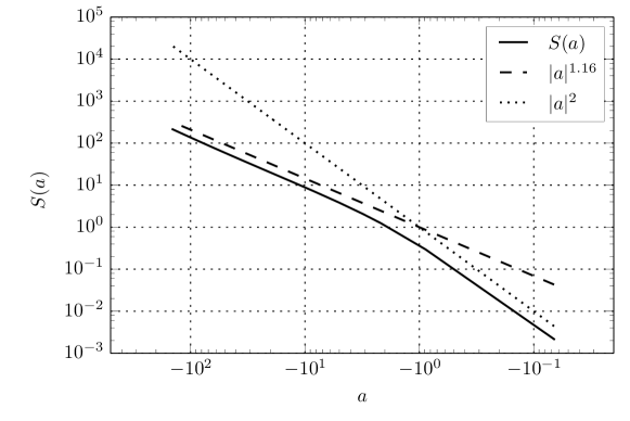
Figure 1: The parameter-free function $S(a)$ computed via solution of the instanton equations (13) shown in log-log scaling for negative values of $a$.

The instanton equations (11) were first integrated numerically in chernykh-stepanov:2001 and later on in grafke-grauer-schaefer:2013 . These calculations turn out to be challenging because the initial condition for $u$ in (12) is set at $t=-\infty$: in practice, we need to set $t=-T$ for some large $T$, and check convergence by varying $T$, but this requires taking larger and larger values of $T$ as $|\lambda|$ increases. To overcome this problem, here we use the approach proposed in grafke-grauer-schaefer-vandeneijnden:2014 building on works in e-ren-vandeneijnden:2004 ; heymann-vandeneijnden:2008 ; heymann-vandeneijnden:2008c ; zhou-ren-e:2008 and solve a reparametrized version of (11) in which the physical time $t\in(-\infty,0]$ is replaced by an artificial, reparametrized time $s\in[-1,0]$ defined in such a way that $\|u_{s}\|_{\chi}=\text{const}$, where $\|v\|_{\chi}=\sqrt{\langle v,v\rangle_{\chi}}$ with $\langle u,v\rangle_{\chi}=\langle u,\chi^{-1}v\rangle$. After reparametrization, the instanton equations (11) become

$$ru_{s}+uu_{x}-u_{xx} =\chi\star p$$ (13)

$$rp_{s}+up_{x}+p_{xx} =0$$

where $r=\|\frac{1}{2}u_{xx}-uu_{x}\|_{\chi}/\|u_{s}\|_{\chi}$, subject to

$$u(s=-1)=0,\qquad p(s=0)=-\lambda\delta^{\prime}(x).$$ (14)

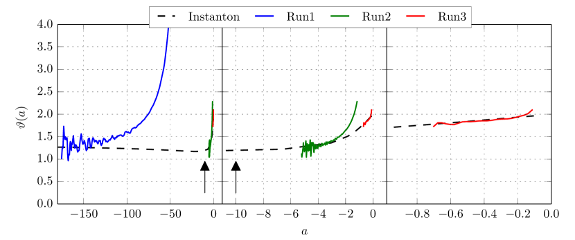
Figure 2: Local exponent $\vartheta(a)$ in (16) obtained from the instanton calculation (dashed line) and compared the values estimated from DNS at the three different values of $\sigma$ summarized in Table 1.

For the numerical simulations presented throughout this paper, we chose

$$\chi(x)=-\partial^{2}_{x}{\mathrm{e}}^{-x^{2}/2}=(1-x^{2}){\mathrm{e}}^{-x^{2}/2}\,.$$ (15)

The instanton equations were solved using a second order explicit integrator in time with a time-step whose size is dictated by the factor $r$ in (13) and can be approximated once for several computations. We used fast Fourier transforms for all spatial derivatives. This scheme was implemented as a GPU/CPU hybrid code for speeding up the computations. The details of its implementation, especially in terms of computational efficiency and reduction of memory requirements, is discussed in grafke-grauer-schindel:2014 . Here we simply note that, because of the mixed initial and final boundary conditions (14), algorithms computing transition probabilities bouchet-laurie-zaboronski:2011 ; e-ren-vandeneijnden:2004 ; heymann-vandeneijnden:2008 with a known initial and final state are not directly applicable in this setup.

	$\sigma$	$l_{d}$	#$T_{L}$
Run1	17.21	0.285	$7.139\cdot 10^{5}$
Run2	1.70	0.909	$9.505\cdot 10^{8}$
Run3	0.52	1.875	$4.266\cdot 10^{6}$

Table 1: Parameters of the DNS at different values of $\sigma$: driving amplitude, $l_{d}=L_{d}/L=\sigma^{-1/2}$: dissipation length, #$T_{L}$: total number of integral times.

The function $S(a)$ obtained by this method confirms the scaling $S(a)\asymp a^{3}$ for large positive values of $a$. Here we focus on large negative values of $a$, where the situation is more complex: $S(a)$ is plotted against $a$ for $a<0$ in Fig. 1 using a log-log scaling. At first glance, it seems like $S(a)\asymp|a|^{2}$ in the core, then switches to $S(a)\asymp|a|^{\vartheta}$ with $\vartheta\approx 1.16$ for larger negative values of $a$. This exponent is not consistent with the theoretical prediction $\vartheta_{\infty}=3/2$ obtained in balkovsky-falkovich-etal:1997 . It is, however, very close to the value $\vartheta=1.15$ that was measured by Gotoh gotoh:1999 in DNS $\textrm{Re}=2$ (i.e. $\sigma\approx 2.83$). To explain the origin of this discrepancy, let us take a closer at the function $S(a)$ and define the local exponent

$$\vartheta(a):=\frac{d\ln S}{d\ln|a|}=\frac{a}{S}\frac{dS}{da}$$ (16)

It can be seen in Fig. 2 that this exponent keeps varying slowly as $a$ decreases to larger negative values, indicating that $S(a)$ is not yet a power-law for the values of $a$ plotted in Fig. 1. In fact, further calculations (not shown) indicates that $\vartheta(a)\to 3/2$ as $a\to-\infty$, consistent with the analytical prediction in balkovsky-falkovich-etal:1997 . This, however, happens for much larger values of $|a|$. At the same time, the arrow in figure 2 denotes the largest negative gradient observed in Gotoh’s DNS simulation Run1, demonstrating that, in fact, his measured value is in remarkable agreement with the instanton prediction for the local exponent at this value of the gradient. Therefore, the results from (gotoh:1999, , Run1) are compatible with the statistics being dominated by instanton-like events, albeit far from the limiting case where the approximation made in balkovsky-falkovich-etal:1997 apply.

This can be further confirmed by comparing these results to our own massive DNS of (3). These simulations were conducted with a total of $2.6\times 10^{11}$ computational steps, amounting to about $10^{9}$ large eddy turnover times in total, for various values of $\sigma$, as summarized in Table 1. The local exponent $\vartheta(a)$ measured in these experiments is also shown in Fig. 2 for three values of $\sigma$. As can been seen, in each cases, the exponent estimated from the DNS eventually approaches the instanton prediction, albeit at values that are not $3/2$. Note the huge range of different gradients captured by this figure.

To assess the range of validity of the instanton predictions, it is useful to plot the gradient PDF estimated from the DNS against $Ce^{-\sigma^{-2}S(a)}$, where the constant $C$ is the normalization factor of the PDF which is lost in the steepest descent calculation. To make this comparison, we also renormalized the driving amplitude $\sigma$ for the more turbulent Run1 and Run2 to account for the fluctuations that are not captured in the instanton calculation: specifically $\sigma_{1}^{\text{eff}}=0.83\sigma_{1}$ and $\sigma_{2}^{\text{eff}}=0.92\sigma_{2}$. The results of these calculations are reported in Fig. 2, where we scaled $u_{x}=a$ by its standard deviation $\sigma$ to make the ranges of the different plots comparable. These graphs show how the tail of the gradient PDF fattens as $\sigma$ increases. They also show that the instanton prediction always matches the estimate from the DNS if $|a|$ is large enough, and the smaller $\sigma$, the larger the range in which agreement is observed. This is consistent with the fact that the estimate in (8) relies on $\sigma^{-2}|\lambda|$ being large, which becomes a more stringent requirement as $\sigma$ (and hence the Reynolds number) increases. At the same time, since the left tail of the gradient PDF fattens as $\sigma$ increases, the instanton prediction does remain relevant to explain intermittency. In fact, if we set $S(a)\sim C|a|^{\vartheta}$ in (8), and assume that $\vartheta$ is roughly constant, we see that the maximum is attained at

$$a_{*}=(\lambda/(C\vartheta))^{1/(\vartheta-1)}\gg(\sigma^{2}/(C\vartheta))^{1/(\vartheta-1)}$$ (17)

where the inequality indicates the range of gradients where the instanton calculation will apply. Since it follows from (3) that the standard deviation of $u_{x}=a$ is $\sigma$, this means that, for large $\sigma$, the instanton method will capture gradients whose amplitude is $\sigma^{(3-\vartheta)/(\vartheta-1)}$ times larger than their standard deviation.

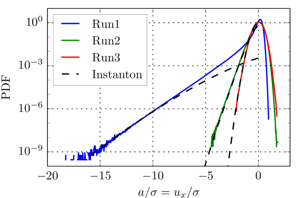
Figure 3: The gradient PDF obtained by the instanton method via $Ce^{-\sigma^{-2}S(a)}$ (dashed lines) is compared to the PDF estimated from DNS (solid lines) at the three different values of $\sigma$ summarized in Table 1.

In conclusion, the instanton approximation is able to reliably predict scaling exponents of the velocity gradient PDF for rare events over a broad range of values. Since the applicability of the method is directly related to the Reynolds number Re, there is little hope of measuring the limiting case of $\vartheta_{\infty}=\frac{3}{2}$ in DNS. Nevertheless, for moderate Re flows the tail scaling can be estimated from the instanton, and for low Re the whole PDF can be derived from the instanton configuration. This also answers the open question raised in gotoh:1999 of the applicability of the instanton approach, and his measured exponent of $\vartheta=1.15$ agrees with our prediction of $\vartheta=1.16$ quite remarkably. The major task for subsequent investigations is to include fluctuations into the presented computations, which would permit predictions for flows with higher Re, and to scale up these calculations to turbulent flows in higher dimensions. Both aims seem achievable.

Acknowledgments: We thank Gregory Falkovich for helpful discussions. The work of T.G. was partially supported through the grants ISF-7101800401 and Minerva – Coop 7114170101. The work of R.G. benefited from partial support through DFG-FOR1048, project B2. The work of T.S. was partially supported by the NSF grant DMS-1108780. The work of E.V.-E. was partially supported by NSF Grant No. DMS07-08140 and ONR Grant No. N00014- 11-1-0345.

References

- (1) J. M. Burgers, The Nonlinear Diffusion Equation. Asymptotic Solutions and Statistical Problems. Dordrecht: Reidel, 1974.
- (2) V. I. Arnol’d, Y. B. Zel’dovich, and S. F. Shandarin, “The large-scale structure of the universe. i. general properties. one-dimensional and two- dimensional models,” Geophys. Astrophys. Fluid Dynam., vol. 20, pp. 111–130, 1982.
- (3) S. F. Shandarin and Y. B. Zel’dovich, “The large-scale structure of the universe: turbulence, intermittency, structures in a self-gravitating medium. 61(2), 185Ð220.,” Rev. Modern Phys., vol. 61, pp. 185–220, 1989.
- (4) D. Chowdhury, L. Santen, and A. Schadschneider, “Statistical physics of vehicular traffic and some related systems,” Phys. Rep., vol. 329, p. 199Ð329, 2000.
- (5) M. Kardar, G. Parisi, and Y.-C. Zhang, “Dynamical scaling of growing interfaces,” Phys. Rev. Lett., vol. 56, pp. 889Ж892, 1986.
- (6) J. Bec and K. Khanin, “Burgers turbulence,” Physics Reports, vol. 447, no. 1, pp. 1–66, 2007.
- (7) U. Frisch, Turbulence. Cambridge: Cambridge University Press, 1995.
- (8) A. M. Polyakov, “Turbulence without pressure,” Phys. Rev. E, vol. 52, pp. 6183–6188, Dec. 1995.
- (9) V. Gurarie and A. Migdal, “Instantons in the Burgers equation,” Phys. Rev. E, vol. 54, p. 4908, 1996.
- (10) W. E, K. Khanin, A. Mazel, and Y. G. Sinai, “Probability distribution functions for the random forced Burgers equation,” Phys. Rev. Lett., vol. 78, p. 1904, 1997.
- (11) T. Gotoh and R. Kraichnan, “Steady-state Burgers turbulence with large-scale forcing,” Physics of Fluids, vol. 10, no. 11, pp. 2859–2866, 1998.
- (12) W. E and E. Vanden Eijnden, “Statistical theory for the stochastic Burgers equation in the inviscid limit,” Communications on Pure and Applied Mathematics, vol. 53, no. 7, pp. 852–901, 2000.
- (13) S. Boldyrev, T. Linde, and A. Polyakov, “Velocity and velocity-difference distributions in Burgers turbulence,” Phys. Rev. Lett., vol. 93, no. 18, 2004.
- (14) T. Gotoh, “Probability density functions in steady-state Burgers turbulence,” Phys. Fluids, vol. 11, pp. 2143–2148, 1999.
- (15) E. Balkovsky, G. Falkovich, I. Kolokolov, and V. Lebedev, “Intermittency of Burgers’ turbulence,” Phys. Rev. Lett., vol. 78, p. 1452, 1997.
- (16) G. Falkovich, I. Kolokolov, V. Lebedev, and A. Migdal, “Instantons and intermittency,” Phys. Rev. E, vol. 54, p. 4896, 1996.
- (17) A. Chernykh and M. Stepanov, “Large negative velocity gradients in Burgers turbulence,” Phys. Rev. E, vol. 64, p. 026306, 2001.
- (18) T. Grafke, R. Grauer, T. Schäfer, and E. Vanden-Eijnden, “Arclength parametrized Hamilton’s equations for the calculation of instantons,” Multiscale Modeling & Simulation, vol. 12, no. 2, pp. 566–580, 2014.
- (19) T. Grafke, R. Grauer, and T. Schäfer, “Instanton filtering for the stochastic Burgers equation,” J. Phys. A: Mathematical and Theoretical, vol. 46, no. 6, p. 62002, 2013.
- (20) P. C. Martin, E. D. Siggia, and H. A. Rose, “Statistical dynamics of classical systems,” Phys. Rev. A, vol. 8, p. 423, 1973.
- (21) C. de Dominicis, “Techniques de renormalisation de la théorie des champs et dynamique des phénomènes critiques,” J. Phys. C, vol. 1, p. 247, 1976.
- (22) H. Janssen, “On a Lagrangian for classical field dynamics and renormalization group calculations of dynamical critical properties,” Z. Physik B, vol. 23, p. 377, 1976.
- (23) S. R. S. Varadhan, “Large deviations,” Ann. Prob., vol. 36, no. 2, pp. 397–419, 2008.
- (24) W. E, W. Ren, and E. Vanden-Eijnden, “Minimum action method for the study of rare events,” Comm. Pure Appl. Math., vol. 57, pp. 1–20, 2004.
- (25) M. Heymann and E. Vanden-Ejnden, “The geometric minimum action method: A least action principle on the space of curves,” Comm. Pure and Appl. Math., vol. 61, p. 1053, 2008.
- (26) M. Heymann and E. Vanden-Eijnden, “Pathways of maximum likelihood for rare events in nonequilibrium systems: application to nucleation in the presence of shear,” Phys. Rev. Lett., vol. 100, no. 14, p. 140601, 2008.
- (27) X. Zhou, W. Ren, and W. E, “Adaptive minimum action method for the study of rare events,” The Journal of chemical physics, vol. 128, p. 104111, 2008.
- (28) T. Grafke, R. Grauer, and S. Schindel, “Efficient computation of instantons for multi-dimensional turbulent flows with large scale forcing,” arXiv:1410.6331 [physics.flu-dyn], Oct. 2014. arXiv: 1410.6331.
- (29) F. Bouchet, J. Laurie, and O. Zaboronski, “Control and instanton trajectories for random transitions in turbulent flows,” J. Phys.: Conf. Ser., vol. 318, p. 022041, 2011.