Reliable Diversity-Based Spatial Crowdsourcing by Moving Workers

Abstract

With the rapid development of mobile devices and the crowdsourcing platforms, the spatial crowdsourcing has attracted much attention from the database community, specifically, spatial crowdsourcing refers to sending a location-based request to workers according to their positions. In this paper, we consider an important spatial crowdsourcing problem, namely reliable diversity-based spatial crowdsourcing (RDB-SC), in which spatial tasks (such as taking videos/photos of a landmark or firework shows, and checking whether or not parking spaces are available) are time-constrained, and workers are moving towards some directions. Our RDB-SC problem is to assign workers to spatial tasks such that the completion reliability and the spatial/temporal diversities of spatial tasks are maximized. We prove that the RDB-SC problem is NP-hard and intractable. Thus, we propose three effective approximation approaches, including greedy, sampling, and divide-and-conquer algorithms. In order to improve the efficiency, we also design an effective cost-model-based index, which can dynamically maintain moving workers and spatial tasks with low cost, and efficiently facilitate the retrieval of RDB-SC answers. Through extensive experiments, we demonstrate the efficiency and effectiveness of our proposed approaches over both real and synthetic datasets.

1 Introduction

Recently, with the ubiquity of smart mobile devices and high-speed wireless networks, people can now easily work as moving sensors to conduct sensing tasks, such as taking photos and recording audios/videos. While data submitted by mobile users often contain spatial-temporal-related information, such as real-world scenes (e.g., street view of Google Maps [1]), video clips (e.g., MediaQ [2]), local hotspots (e.g., Foursquare [3]), and traffic conditions (e.g., Waze [4]), the spatial crowdsourcing platform [18, 20] has nowadays drawn much attention from both academia (e.g., the database community) and industry (e.g., Amazon’s AMT [5]).

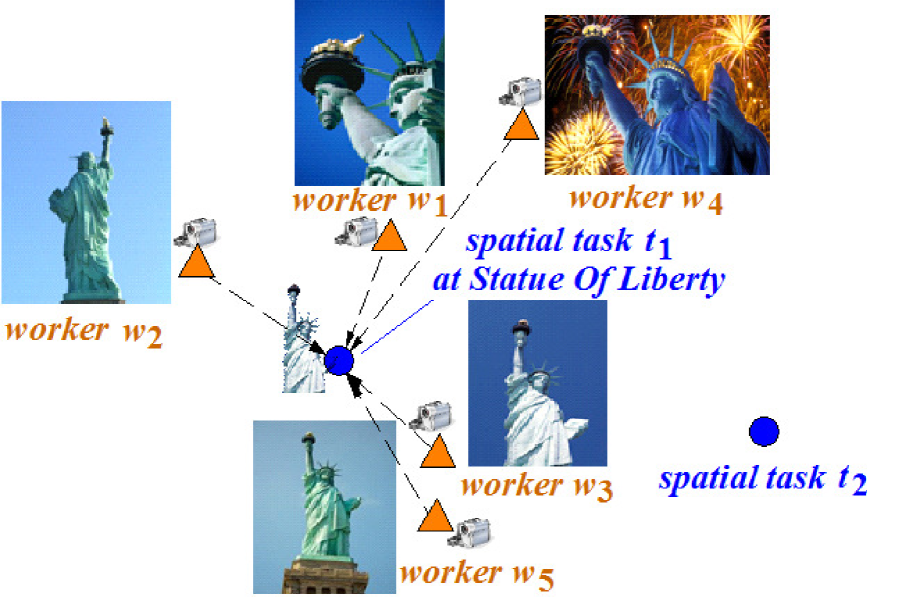
Figure 1: An Example of Taking Photos/Videos of a Landmark (Statue of Liberty) in the Spatial Crowdsourcing System.

Specifically, a spatial crowdsourcing platform [18, 20] is in charge of assigning a number of workers to nearby spatial tasks, such that workers need to physically move towards some specified locations to finish tasks (e.g., taking photos/videos).

Example 1 (Taking Photos/Videos of a Landmark). Consider a scenario of the spatial crowdsourcing in Figure 1, in which there are two spatial tasks at locations $t_{1}$ and $t_{2}$, and 5 workers, $w_{1}\sim w_{5}$. In particular, the spatial task $t_{1}$ is for workers to take 2D photos/videos of a landmark, the Statue of Liberty, while walking from ones’ current locations towards it. The resulting 2D photos/videos are useful for real applications such as virtual tours and 3D landmark reconstruction. Therefore, the task requester is usually interested in obtaining a full view of the landmark from diverse directions (e.g., photos from the back of the statue that not many people saw before).

As shown in Figure 1, workers $w_{1}$ and $w_{4}$ can take photos from left hand side of the statue, worker $w_{2}$ can take photos from the back of the statue, and workers $w_{3}$ and $w_{5}$ can take photos from the front of the statue. Since photos/videos from similar directions are not informative for the 3D reconstruction or virtual tours, the spatial crowdsourcing system needs to select those workers who can take photos of the statue with as diverse directions as possible, and then assign task $t_{1}$ to them.

Note that, when worker $w_{4}$ arrives at the location of $t_{1}$, he can take a photo of the landmark at night with fireworks. As a result, by assigning task $t_{1}$ to worker $w_{4}$, we can obtain a quite diverse photo at night for virtual tours, compared with that taken by worker $w_{1}$ in the daytime (even though they are taken from similar angles). Thus, it is also important to consider the temporal diversity of taking the photos, in terms of the arrival times of workers at $t_{1}$.   $\blacksquare$

Example 2 (Available Parking Space Monitoring over a Region). In the application of monitoring free parking spaces in a spatial region, it is important to analyze the photos taken from diverse directions and at different time periods of the day, and predict the trend of available parking spaces in the future. This is because some available parking spaces might be hidden by other cars for photos just from one single direction (or multiple similar directions), and moreover, photos taken at different timestamps have richer information than those taken at a single time point, for the purpose of predicting the availability of parking spaces. Therefore, in this case, the spatial crowdsourcing system needs to assign such a task to those workers with diverse walking directions to it and arrival times.   $\blacksquare$

In this paper, we will investigate a realistic scenario of spatial crowdsourcing, where workers are dynamically moving towards some directions, and spatial tasks are constrained by valid time periods. For example, a worker may want to do spatial tasks on the way home, and thus he/she tends to accept tasks only along the direction to home, rather than an opposite direction. Similarly, a spatial task of taking photos of the statue, together with fireworks, is restricted by the period of the firework show time. Therefore, a worker can only conduct a task within the constrained time range and prefer to accepting the tasks close to his/her moving direction. In this paper, we characterize features of moving workers and time-constrained spatial tasks, which have not been studied before.

Under the aforementioned realistic scenario, we propose the problem of dynamic task-and-worker assignment, by considering the answer quality of spatial tasks, in terms of two measures: spatial-temporal diversities and reliability. In particular, inspired by the two applications above (Examples 1 and 2), for spatial tasks, photos/videos from diverse angles or timestamps can provide a comprehensive view of the landmark, which is more preferable than those taken from a single boring direction/time; similarly, photos taken by different directions and periods are more useful for the trend prediction of available parking spaces. Therefore, in this paper, we will introduce the concepts of spatial diversity and temporal diversity to spatial crowdsourcing, which capture the diversity quality of the returned answers (e.g., photos taken from different angles and at different timestamps) to spatial tasks.

Furthermore, in reality, it is possible that answers provided by workers are not always correct, for example, the uploaded photos/videos might be fake ones, or workers may deny the assigned tasks. Thus, we will model the confidence of each worker, and in turn, guarantee high reliability of each spatial task, which is defined as the confidence that at least one worker assigned to this task can give a high quality answer.

Note that, while existing works on spatial crowdsourcing [18, 20] focused on the assignment of workers and tasks to maximize the total number of completed tasks, they did not consider much about the constrained features of workers/tasks (workers’ moving directions and tasks’ time constraints). Most importantly, they did not take into account the quality of the returned answers.

By considering both quality measures of spatial-temporal diversities and reliability, in this paper, we will formalize the problem of reliable diversity-based spatial crowdsourcing (RDB-SC), which aims to assign moving workers to time-constrained spatial tasks such that both reliability and diversity are maximized. To the best of our knowledge, there are no previous works that study reliability and spatial/temporal diversities in the spatial crowdsourcing. However, efficient processing of the RDB-SC problem is quite challenging. In particular, we will prove that the RDB-SC problem is NP-hard, and thus intractable. Therefore, we propose three approximation approaches, that is, the greedy, sampling, and divide-and-conquer algorithms, in order to efficiently tackle the RDB-SC problem. Furthermore, to improve the time efficiency, we design a cost-model-based index to dynamically maintain moving workers and time-constrained spatial tasks, and efficiently facilitate the dynamic assignment in the spatial crowdsourcing system. Finally, through extensive experiments, we demonstrate the efficiency and effectiveness of our approaches.

To summarize, we make the following contributions.

• We formally propose the problem of reliable diversity-based spatial crowdsourcing (RDB-SC) in Section 2, by introducing the reliability and diversity to guarantee the quality of spatial tasks.

• We prove that the RDB-SC problem is NP-hard, and thus intractable in Section 3.

• We propose three approximation approaches, greedy, sampling, and divide-and-conquer algorithms, in Sections 4, 5 and 6, respectively, to tackle the RDB-SC problem.

• We conduct extensive experiments in Section 8 on both real and synthetic datasets and show the efficiency and effectiveness of our approaches.

We design a cost-model-based index structure to dynamically maintain workers and tasks in Section 7. Section 9 overviews previous works on (spatial) crowdsourcing. Finally, Section 10 concludes this paper.

2 Problem Definition

2.1 Time-Constrained Spatial Tasks

We first define the time-constrained spatial tasks in the crowdsourcing applications.

Definition 1

$($Time-Constrained Spatial Tasks$)$ Let $T=\{t_{1},$ $t_{2},...,t_{m}\}$ be a set of $m$ time-constrained spatial tasks. Each spatial task $t_{i}$ ($1\leq i\leq m$) is located at a specific location $l_{i}$, and associated with a valid time period $[s_{i},e_{i}]$.   $\blacksquare$

In this paper, we consider spatial and time-constrained tasks, such as “taking 2D photos/videos for the Statue of Liberty together with fireworks”, or “taking photos of parking places during open hours of the parking area in a region”. Therefore, in such scenarios, each task can only be accomplished at a specific location, and, moreover, satisfy the time constraint. For example, photos should be taken by people in person and within the period of the firework show. Therefore, in Definition 1, we require each spatial task $t_{i}$ be accomplished at a spatial location $l_{i}$ (for $1\leq i\leq m$), and within a valid period $[s_{i},e_{i}]$.

The set of spatial tasks is dynamically changing. That is, the newly created tasks keep on arriving, and those completed (or expired) tasks are removed from the crowdsourcing system.

2.2 Dynamically Moving Workers

Next, we consider dynamically moving workers.

Definition 2

$($Dynamically Moving Workers$)$ Let $W=\{w_{1},$ $w_{2},$ $...,w_{n}\}$ be a set of $n$ workers. Each worker $w_{j}$ ($1\leq j\leq n$) is currently located at position $l_{j}$, moving with velocity $v_{j}$, and towards the direction with angle $\alpha_{j}\in[\alpha_{j}^{-},\alpha_{j}^{+}]$. Each worker $w_{j}$ is associated with a confidence $p_{j}\in[0,1]$, which indicates the reliability of the worker that can do the task.

$\blacksquare$

Intuitively, a worker $w_{j}$ ($1\leq j\leq n$) may want to do tasks on the way to some place during the trip. Thus, as mentioned in Definition 2, the worker can pre-register the angle range, $[\alpha_{j}^{-},\alpha_{j}^{+}]$, of one’s current moving direction. In other words, the worker is only willing to accomplish tasks that do not deviate from his/her moving direction significantly. For other (inconvenient) tasks (e.g., opposite to the moving direction), the worker tends to ignore/reject the task request, thus, the system would not assign such tasks to this worker. In the case that the worker has no targeting destinations (i.e., free to move), he/she can set $[\alpha_{j}^{-},\alpha_{j}^{+}]$ to $[0,2\pi]$.

After being assigned with a spatial task, a worker sometimes may not be able to finish the task. For example, the worker might reject the task request (e.g., due to other tasks with higher prices), do the task incorrectly (e.g., taking a wrong photo), or miss the deadline of the task. Thus, as given in Definition 2, each worker $w_{j}$ is associated with a confidence $p_{j}\in[0,1]$, which is the probability (or reliability) that $w_{j}$ can successfully finish a task (inferred from historical data of this worker). In this paper, we consider the model of server assigned tasks (SAT) [20]. That is, we assume that once a worker accepts the assigned task, the worker will voluntarily do the task. Similar to spatial tasks, workers can freely register or leave the crowdsourcing system. Thus, the set of workers is also dynamically changing.

2.3 Reliable Diversity-Based Spatial Crowdsourcing

With the definitions of tasks and workers, we are now ready to formalize our spatial crowdsourcing problem (namely, RDB-SC), which assigns dynamically moving workers to time-constrained spatial tasks with high accuracy and quality.

Before we provide the formal problem definition, we first quantify the criteria of our task assignment during the crowdsourcing, in terms of two measures, the reliability and spatial/temporal diversity. The reliability indicates the confidence that at least some worker can successfully complete the task, whereas the spatial/temporal diversity reflects the quality of the task accomplishment by a group of workers, in both spatial and temporal dimensions (e.g., taking photos from diverse angles and at diverse timestamps).

Reliability. Since not all workers are trustable, we should consider the reliability, $p_{j}$, of each workers, $w_{j}$, during the task assignment. For example, some workers might take a wrong photo, or fail to reach the task location before the valid period. In such cases, the goal of our task assignment is to guarantee that tasks $t_{i}$ can be accomplished by those assigned workers with high confidence.

Definition 3

$($Reliability$)$ Given a spatial task $t_{i}$ and its assigned set, $W_{i}$, of workers, the reliability, $rel(t_{i},W_{i})$, of a worker assignment w.r.t. $t_{i}$ is given by:

$$rel(t_{i},W_{i})=1-\prod_{\forall w_{j}\in W_{i}}(1-p_{j}).$$ (1)

where $p_{j}$ is the probability that worker $w_{j}$ can reliably complete task $t_{i}$.   $\blacksquare$

Intuitively, Eq. (1) gives the probability (reliability) that there exists some worker who can accomplish the task $t_{i}$ reliably (e.g., taking the right photo, or providing a reliable answer). In particular, the second term (i.e., $\prod_{\forall w_{j}\in W_{i}}(1-p_{j})$) in Eq. (1) is the probability that all the assigned workers in $W_{i}$ cannot finish the task $t_{i}$. Thus, $1-\prod_{\forall w_{j}\in W_{i}}(1-p_{j})$ is the probability that task $t_{i}$ can be completed by at least one assigned worker in $W_{i}$.

High reliability usually leads to good confidence of the task completion. In this paper, we aim to maximize the reliability for each individual task.

Possible Worlds of the Task Completion. Since not all the assigned workers in $W_{i}$ can complete the task $t_{i}$, it is possible that only a subset of workers in $W_{i}$ can succeed in accomplishing the task $t_{i}$ in the real world. In practice, there are an exponential number (i.e., $O(2^{|W_{i}})$) of such possible subsets.

Following the literature of probabilistic databases [17], we call each possible subset in $W_{i}$ a possible world, denoted as $pw(W_{i})$, which contains those workers who may finish the task $t_{i}$ in reality. Each possible world, $pw(W_{i})$, is associated with a probability confidence,

$$Pr\{pw(W_{i})\}=\prod_{\forall w_{j}\in pw(W_{i})}p_{j}\cdot\prod_{\forall w_{j}\in(W_{i}-pw(W_{i}))}(1-p_{j}),$$ (2)

which is given by multiplying probabilities that workers in $W_{i}$ appear or do not appear in the possible world $pw(W_{i})$.

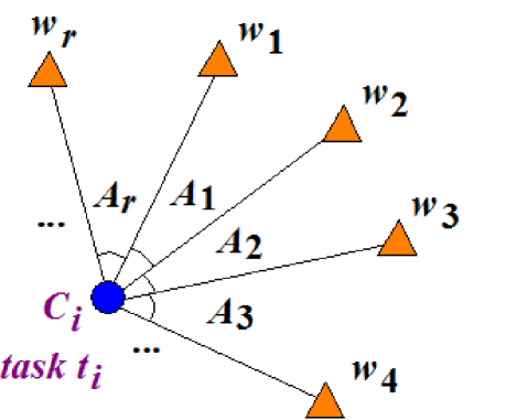
(a) Spatial Diversity

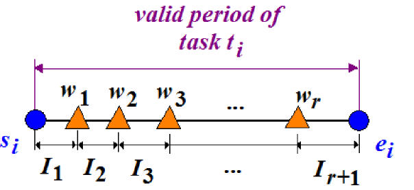
(b) Temporal Diversity

Figure 2: Illustration of Spatial/Temporal Diversity.

Spatial/Temporal Diversity. As mentioned in Example 1 of Section 1 (i.e., take photos of a statue), it would be nice to obtain photos from different angles and at diverse times of the day, and get the full picture of the statue for virtual tours. Similarly, in Example 2 (Section 1), it is desirable to obtain photos of parking areas from different directions at diverse times, in order to collect/analyze data of available parking spaces during open hours. Thus, we want workers to accomplish spatial tasks (e.g., taking photos) from different angles and over timestamps as diverse as possible. We quantify the quality of the task completion by spatial/temporal diversities.

Specifically, the spatial diversity (SD) is defined as follows. As illustrated in Figure 2(a), let $C_{i}$ be a point at the location $l_{i}$ (or the centroid of a region) of task $t_{i}$. Assume that $r$ workers $w_{j}\in W_{i}$ ($1\leq j\leq r$) do tasks (i.e., take pictures) at $l_{i}$ from different angles. We draw $r$ rays from $C_{i}$ to the directions of $r$ workers who take photos. Then, with these $r$ rays, we can obtain $r$ angles, denoted as $A_{1}$, $A_{2}$, …, and $A_{r}$, where $\sum_{j=1}^{r}A_{j}=2\pi$. Intuitively, the entropy was used as an expression of the disorder, or randomness of a system. Here, higher diversity indicates more discorder, which can be exactly captured by the entropy. That is, when the answers come from diverse angles and timestamps, the answers have high entropy. Thus, we use the entropy to define the spatial diversity (SD) as follows:

$$SD(t_{i})=-\sum_{j=1}^{r}\frac{A_{j}}{2\pi}\cdot log\left(\frac{A_{j}}{2\pi}\right)$$ (3)

Similarly, we can give the temporal diversity for the arrival times of workers (to do tasks), by using the entropy of time intervals. As shown in Figure 2(b), assume that the arrival times of $r$ workers divide the valid period $[s_{i},e_{i}]$ of task $t_{i}$ into $(r+1)$ sub-intervals of lengths $I_{1}$, $I_{2}$, …, and $I_{r+1}$. We define the temporal diversity (TD) below:

$$TD(t_{i})=-\sum_{j=1}^{r+1}\frac{I_{j}}{e_{i}-s_{i}}\cdot log\left(\frac{I_{j}}{e_{i}-s_{i}}\right)$$ (4)

Intuitively, larger SD or TD value indicates higher diversity of spatial angles or time distribution, which is more desirable by task requesters. We combine these 2 diversity types, and obtain the spatial/temporal diversity (STD) w.r.t. $W_{i}$, below:

$$STD(t_{i},W_{i})=\beta\cdot SD(t_{i})+(1-\beta)\cdot TD(t_{i}),$$ (5)

where parameter $\beta\in[0,1]$. Here, $\beta$ is a weight balancing between SD and TD, which depends on the application requirement specified by the task requester of $t_{i}$. When $\beta=0$, we consider TD only; when $\beta=1$, we require SD only in the spatial task $t_{i}$.

Therefore, under possible worlds semantics, in this paper, we will consider the expected spatial/temporal diversity (defined later) in our crowdsourcing problem.

The RDB-SC Problem. We define our RDB-SC problem below.

Definition 4

$($Reliable Diversity-Based Spatial Crowdsourcing, RDB-SC$)$ Given $m$ time-constrained spatial tasks in $T$, and $n$ dynamically moving workers in $W$, the problem of reliable diversity-based spatial crowdsourcing (RDB-SC) is to assign each task $t_{i}\in T$ with a set, $W_{i}$, of workers $w_{j}\in W$, such that:

1. each worker $w_{j}\in W$ is assigned with a spatial task $t_{i}\in T$ such that his/her arrival time at location $l_{i}$ falls into the valid period $[s_{i},e_{i}]$,

2. the minimum reliability, $\min_{i=1}^{m}rel(t_{i},W_{i})$, of all tasks $t_{i}$ is maximized, and

3. the summation, $total\_STD$, of the expected spatial/temporal diversities, $E(STD(t_{i}))$, for all tasks $t_{i}$, is maximized,

where the expected spatial/temporal diversity $E(STD(t_{i}))$ is:

$$E(STD(t_{i}))=\sum_{\forall pw(W_{i})}Pr\{pw(W_{i})\}\cdot STD(t_{i},pw(W_{i})),\text{ and}\vspace{-3ex}$$ (6)

$$total\_STD=\sum_{i=1}^{m}E(STD(t_{i})).$$ (7)

The RDB-SC problem is to assign workers to collaboratively accomplish each task with two optimization goals: (1) the smallest reliability among all tasks is maximized (intuitively, if the smallest reliability of tasks is maximized, then the reliability of all tasks must be high), and (2) the summed expected diversity for all tasks is maximized. These two goals aim to guarantee the confidence of the task completion and the diversity quality of the tasks, respectively.

Answer Aggregation for a Spatial Task. After assigning a set, $W_{i}$, of workers to spatial task $t_{i}$, we can obtain a set of answers, for example, photos in Example 1 of Section 1 with different angles and at diverse timestamps. It is also important to present these photos to the task requester. Due to too many photos, we can apply aggregation techniques to group those photos with similar spatial/temporal diversities, and show the task requester only one representative photo from each group. Moreover, since we consider taking photos as tasks, the task requester can choose the photos with high quality (e.g., resolution or sharpness) from all the answers if he/she wants to. This is, however, not the focus of this paper, and we would like to leave it as future work.

2.4 Challenges

According to Definition 4, the RDB-SC problem is an optimization problem with two objectives. The challenges of tackling the RDB-SC problem are threefold. First, with $m$ time-constrained spatial tasks and $n$ moving workers, in the worst case, there are an exponential number of possible task-worker assignment strategies, that is, with time complexity $O(m^{n})$. In fact, we will later prove that the RDB-SC problem is NP-hard. Thus, it is inefficient or even infeasible to enumerate all possible assignment strategies.

Second, the second objective in the RDB-SC problem considers maximizing the summed expected spatial/temporal diversities, which involves an exponential number of possible worlds for diversity computations. That is, the time complexity of enumerating possible worlds is $O(2^{|W_{i}|})$, where $W_{i}$ is a set of assigned workers to task $t_{i}$. Therefore, it is not efficient to compute the spatial/temporal diversity by taking into account all possible worlds.

Third, in the RDB-SC problem, workers move towards some directions, whereas spatial tasks are restricted by time constraints (i.e., valid period $[s_{i},e_{i}]$). Both workers and tasks can enter/quit the spatial crowdsourcing system dynamically. Thus, it is also challenging to dynamically decide the task-worker assignment.

Inspired by the challenges above, in this paper, we first prove that the RDB-SC problem is NP-hard, and design three efficient approximation algorithms, which are based on greedy, sampling, and divide-and-conquer approaches. To tackle the second challenge, we reduce the computation of the expected diversity under possible worlds semantics to the one with cubic cost, which can greatly improve the problem efficiency. Finally, to handle the cases that workers and tasks can dynamically join and leave the system freely, we design effective grid index to enable dynamic updates of worker/tasks, as well as the retrieval of assignment pairs.

Table 1 summarizes the commonly used symbols.

Table 1: Symbols and descriptions.

Symbol	Description
$T$	a set of $m$ time-constrained spatial tasks $t_{i}$
$W$	a set of $n$ dynamically moving workers $w_{j}$
$[s_{i},e_{i}]$	the time constraint of accomplishing a task $t_{i}$
$l_{i}$ (or $l_{j}$)	the position of task $t_{i}$ (or worker $w_{j}$)
$v_{j}$	the velocity of moving worker $w_{j}$
$p_{j}$	the confidence of worker $w_{j}$ that reliably do the task
$[\alpha_{j}^{-},\alpha_{j}^{+}]$	the interval of moving direction (angle)
$rel(t_{i},W_{i})$	the reliability that task $t_{i}$ can be completed by workers in $W_{i}$
$R(t_{i},W_{i})$	a (equivalent) variant of reliability $rel(t_{i},W_{i})$
$STD(t_{i},W_{i})$	the spatial/temporal diversity of task $t_{i}$
$E(STD(t_{i}))$	the expected spatial/temporal diversity of task $t_{i}$
$total\_STD$	the sum of the expected spatial/temporal diversities for all tasks
$K$	the sample size

3 Problem Reduction

3.1 Reduction of Reliability

As mentioned in Definition 4, the first optimization goal of the RDB-SC problem is to maximize the minimum reliability among $m$ tasks. Since it holds that the reliability $rel(t_{i},W_{i})=1-\prod_{w_{j}\in W_{i}}(1-p_{j})$ (given in Eq. (1)), we can rewrite it as:

$$R(t_{i},W_{i})=-ln(1-rel(t_{i},W_{i}))=\sum_{w_{j}\in W_{i}}-ln(1-p_{j}).$$ (8)

From Eq. (8), our goal (w.r.t. reliability) of maximizing the smallest $rel(t_{i},W_{i})$ for all tasks $t_{i}$ is equivalent to maximizing the smallest $-ln(1-rel(t_{i},W_{i}))$ (i.e., LHS of Eq. (8)) for all $t_{i}$. In turn, we can maximize the smallest $\sum_{w_{j}\in W_{i}}-ln(1-p_{j})$ (i.e., RHS of Eq. (8)) among all tasks.

Intuitively, we associate each worker $w_{j}$ with a positive constant $-ln(1-p_{j})$. Then, we divide $n$ workers into $m$ disjoint partitions (subsets) $W_{i}$ ($1\leq i\leq n$), and each subset $W_{i}$ has a summed value $\sum_{w_{j}\in W_{i}}-ln(1-p_{j})$ (i.e., RHS of Eq. (8)). As a result, our equivalent reliability goal is to find a partitioning strategy such that the smallest summed value among $m$ subsets is maximized.

3.2 Reduction of Diversity

As discussed in Section 2.4, the direct computation of the expected diversity involves an exponential number of possible worlds $pw(W_{i})$ (see Eq. (6)). It is thus not efficient to enumerate all possible worlds. In this subsection, we will reduce such a computation to the problem with polynomial cost.

Specifically, in order to compute the expected spatial diversity, $E(SD(t_{i}))$, of a task $t_{i}$, we introduce a spatial diversity matrix, $M_{SD}$, in which each entry $M_{SD}[j][k]$ stores a value, given by the multiplication of the probability that an angle $A_{j,k}=(\sum_{x=j}^{k+r}A_{(x\%r)})\%2\pi$ exists (in possible worlds) and entropy $-(\frac{A_{j,k}}{2\pi})\cdot log(\frac{A_{j,k}}{2\pi})$, where $x\%y$ is $x$ mod $y$.

In particular, we have:

$$M_{SD}[j][k]=-(\frac{A_{j,k}}{2\pi})\cdot log(\frac{A_{j,k}}{2\pi})\cdot p_{j}\cdot p_{k}\cdot\prod_{x=j+1}^{(k+r-1)\%r}(1-p_{x}).$$ (9)

The time complexity of computing $M_{SD}[j][k]$ is $O(r)$. Thus, the total cost of spatial diversity matrix is $O(r^{3})$.

Similarly we can compute the temporal diversity matrix, $M_{TD}$, in which each entry $M_{TD}[j][k]$ ($j\leq k$) is given by the multiplication of the probability that a time interval $I_{j,k}=\bigcup_{x=j}^{k}I_{x}$ exists in possible worlds and entropy $-(\frac{I_{j,k}}{e_{i}-s_{i}})\cdot log(\frac{I_{j,k}}{e_{i}-s_{i}})$, for $j\leq k$; moreover, $M_{TD}[j][k]=0$,if $j>k$.

Formally, for $j\leq k$, we have:

$$M_{TD}[j][k]=-(\frac{I_{j,k}}{e_{i}-s_{i}})\cdot log(\frac{I_{j,k}}{e_{i}-s_{i}})\cdot p_{k}\cdot\prod_{x=j+1}^{(k-1)}(1-p_{x}).$$ (10)

To compute $E(STD(t_{i}))$, the expected spatial/temporal diversity, we have the following lemma.

Lemma 3.1

(Expected Spatial/Temporal Diversity) The expected spatial/temporal diversity, $E(STD(t_{i}))$, of task $t_{i}$ is given by:

$$E(STD(t_{i})) = \beta\cdot E(SD(t_{i}))+(1-\beta)\cdot E(TD(t_{i}))$$

$$= \beta\cdot\sum_{\forall j,k}M_{SD}[j][k]+(1-\beta)\cdot\sum_{\forall j,k}M_{TD}[j][k].$$

Proof 3.1.

Please refer to Appendix A of the technical report [6].

In this subsection, we prove that the hardness of our RDB-SC problem is NP-hard. Specifically, we can reduce the problem of the number partition problem [21] (which is known to be an NP-hard problem) to our RDB-SC problem. This way, our RDB-SC problem is also an NP-hard problem:

Lemma 3.2.

(Hardness of the RDB-SC Problem) The problem of the reliable diversity-based spatial crowdsourcing (RDB-SC) is NP-hard.

Proof 3.3.

Please refer to Appendix B of the technical report [6].

From Lemma 3.2, we can see that the RDB-SC problem is not tractable. Therefore, in the sequel, we aim to propose approximation algorithms to find suboptimal solution efficiently.

4 The Greedy Approach

4.1 Properties of Optimization Goals

In this subsection, we provide the properties about the reliability and the expected spatial/temporal diversity. Specifically, assume that a task $t_{i}$ is assigned with a set, $W_{i}$, of $r$ workers $w_{j}$ ($1\leq j\leq r$). Let $w_{r+1}$ be a new worker (with confidence $p_{r+1}$ who is also assigned to task $t_{i}$.

Reliability. We first give the property of the reliability upon a newly assigned worker.

Lemma 4.1.

(Property of the Reliability) Let $R(t_{i},W_{i})$ be the reliability of task $t_{i}$ (given in Eq. (8), in the reduced goal of Section 3.1), associated with a set, $W_{i}$, of $r$ workers. If a new worker $w_{r+1}$ is assigned to $t_{i}$, then we have:

$$R(t_{i},W_{i}\cup\{w_{r+1}\})=R(t_{i},W_{i})-ln(1-p_{r+1}).$$ (12)

Proof 4.2.

Please refer to Appendix C of the technical report [6].

From Eq. (12) in Lemma 4.1, we can see that the second term (i.e., $-ln(1-p_{r+1})$) is a positive value. Thus, it indicates that when we assign more workers (e.g., $w_{r+1}$ with confidence $p_{r+1}\leq 0$) to task $t_{i}$, the reliability, $R(t_{i},\cdot)$, of the task $t_{i}$ is always increasing (at least non-decreasing).

Diversity. Next, we give the property of the expected spatial/temporal diversity, upon a newly assigned worker.

Lemma 4.3.

(Property of the Expected Spatial/Temporal Diversity) Let $E(STD(t_{i}))$ be the expected spatial/temporal diversity of task $t_{i}$. Upon a newly assigned worker $w_{r+1}$ with confidence $p_{r+1}$, the expected diversity $E(STD(t_{i}))$ of task $t_{i}$ is always non-decreasing, that is, $E(STD(t_{i},W_{i}\cup\{w_{r+1}\}))\geq E(STD(t_{i},W_{i}))$.

Proof 4.4.

Please refer to Appendix D of the technical report [6].

Lemma 4.3 indicates that when we assign a new worker to a spatial task $t_{i}$, the expected spatial/temporal diversity is non-decreasing.

Procedure RDB-SC_Greedy { Input: $m$ time-constrained spatial tasks in $T$ and $n$ workers in $W$ Output: a task-and-worker assignment strategy, $\mathbb{S}$, with high reliability and diversity (1) $\mathbb{S}=\emptyset$ (2) compute all the valid task-and-worker pairs $(t_{i},w_{j})$ (3) for $i=1$ to $n$ // in each round, select one best task-and-worker pair (4) for each pair $(t_{i},w_{j})$ ($w_{j}\in W$) (5) compute the increase pair ($\Delta R(t_{i},w_{j}),\Delta STD(t_{i},w_{j})$) (6) prune ($\Delta R(t_{i},w_{j}),\Delta STD(t_{i},w_{j})$) dominated by others (7) rank the remaining pairs by their scores (i.e., the number of dominated pairs) (8) select a pair, $(t_{i},w_{j})$, with the highest score and add it to $\mathbb{S}$ (9) $W=W-\{w_{j}\}$ (10) return $\mathbb{S}$ }

Figure 3: RDB-SC Greedy Algorithm.

4.2 The Greedy Algorithm

As mentioned in Section 4.1, when we assign more workers to a spatial task, the reliability and diversity of the assignment strategy is always non-decreasing. Based on these properties, we propose a greedy algorithm, which iteratively assigns workers to spatial tasks that can always achieve high ranks (w.r.t. reliability and diversity).

Figure 3 illustrates the pseudo code of our RDB-SC greedy algorithm, namely RDB-SC_Greedy, which returns one best strategy, $\mathbb{S}$, containing task-and-worker assignments with high reliability and diversity. Specifically, our greedy algorithm iteratively finds one pair of task and worker such that the assignment with this pair can increase the reliability and diversity most.

Initially, there is no task-and-worker assignment, thus, we set $\mathbb{S}$ to empty (line 1). Next, we identify all the valid task-and-worker pairs $(t_{i},w_{j})$ in the crowdsourcing system (line 2). Here, the validity of pair $(t_{i},w_{j})$ means that worker $w_{j}$ can reach the location of task $t_{i}$, under the constraints of both moving directions and valid period. Then, among these pairs, we want to incrementally select $n$ best task-and-worker assignments such that the increases of reliability and diversity are always maximized (lines 3-9).

In particular, in each iteration, for every task-and-worker pair $(t_{i},w_{j})$ ($w_{j}\in W$ is a worker who has no task), if we allow the assignment of worker $w_{j}$ to $t_{i}$, we can calculate the increases of the reliability and diversity ($\Delta R(t_{i},w_{j}),\Delta STD(t_{i},$ $w_{j})$) (lines 4-5), where $\Delta R(t_{i},w_{j})=R(\mathbb{S}\cup\{(t_{i},w_{j}\})-R(\mathbb{S})$, and $\Delta STD(t_{i},w_{j})=STD(\mathbb{S}\cup\{(t_{i},w_{j}\})-STD(\mathbb{S})$. Note that, as guaranteed by Lemmas 4.1 and 4.3, here the two optimization goals are always non-decreasing (i.e., $\Delta R(\cdot)$ and $\Delta STD(\cdot)$ are positive).

Since some increase pairs may be dominated [13] by others, we can safely filter out such false alarms with both lower reliability and diversity (line 6). We say assignment $\mathbb{S}_{i}$ dominates $\mathbb{S}_{j}$ when $R(\mathbb{S}_{i})>R(\mathbb{S}_{j})$ and $STD(\mathbb{S}_{i})\geq STD(\mathbb{S}_{j})$, or $R(\mathbb{S}_{i})\geq R(\mathbb{S}_{j})$ and $STD(\mathbb{S}_{i})>STD(\mathbb{S}_{j})$. If there are more than one remaining pair, we rank them according to the number of pairs that they are dominating [22] (line 7). Intuitively, the pair (i.e., assignment) with higher rank indicates that this assignment is better than more other assignments. Thus, we add a pair $(t_{i},w_{j})$ with the highest rank to $\mathbb{S}$, and remove the worker $w_{j}$ from $W$ (lines 8-9).

The selection of pairs (assignments) repeats for $n$ rounds (line 3). In each round, we find one assignment pair that can locally increase the maximum reliability and diversity. Finally, we return $\mathbb{S}$ as the best RDB-SC assignment strategy (line 10).

The Time Complexity. The time complexity of computing the best task-and-worker pair in each iteration is given by $O(m\cdot n)$ in the worst case (i.e., each of $n$ worker can be assigned to any of the $m$ tasks). Since we only need to select $n$ task-and-worker pairs (each worker can only be assigned to one task at a time), the total time complexity of our greedy algorithm is given by $O(m\cdot n^{2})$.

4.3 Pruning Strategies

Note that, to compute the exact increase of the reliability $R(t_{i},W_{i})$, we can immediately obtain the reliability increase of task $t_{i}$: $\Delta R(t_{i},$ $w_{j})=-ln(1-p_{j})$. For the diversity, however, it is not efficient to compute the exact increase, $\Delta STD(t_{i},w_{j})$, since we need to update the diversity matrices (as mentioned in Section 3.2) before/after the worker insertion. Therefore, in this subsection, we present an effective pruning method to reduce the search space without calculating the expected diversity for every $(t_{i},w_{j})$ pair.

Our basic idea of the pruning method is as follows. For any task-and-worker pair $(t_{i},w_{j})$, assume that we can quickly compute its lower and upper bounds of the increase for the expected spatial/temporal diversity, denoted as $lb\_\Delta D(t_{i},w_{j})$ and $ub\_\Delta D(t_{i},$ $w_{j})$, respectively.

Then, for two pairs $(t_{i},w_{j})$ and $(t_{i}^{\prime},w_{j}^{\prime})$, if it holds that $lb\_\Delta D(t_{i},$ $w_{j})>ub\_\Delta D(t_{i}^{\prime},w_{j}^{\prime})$, then the diversity increase of pair $(t_{i}^{\prime},w_{j}^{\prime})$ is inferior to that of pair $(t_{i},w_{j})$.

We have the pruning lemma below.

Lemma 4.5.

(Pruning Strategy) Assume that $lb\_\Delta D(t_{i},w_{j})$ and $ub\_\Delta D(t_{i},$ $w_{j})$ are lower and upper bounds of the increase for the expected spatial/temporal diversity, respectively. Similarly, let $\Delta min\_R(t_{i},w_{j})$ be the increase of the smallest reliability among $m$ tasks after assigning worker $w_{i}$ to $t_{i})$, respectively. Then, given two pairs $(t_{i},w_{j})$ and $(t_{i}^{\prime},w_{j}^{\prime})$, if it holds that: (1) $\Delta min\_R(t_{i},w_{j})\\ \geq\Delta min\_R(t_{i}^{\prime},w_{j}^{\prime})$, and (2) $lb\_\Delta D(t_{i},w_{j})>ub\_\Delta D(t_{i}^{\prime},w_{j}^{\prime})$, then we can safely prune the pair $(t_{i}^{\prime},w_{j}^{\prime})$.

Proof 4.6.

Please refer to Appendix E of the technical report [6].

The Computation of Lower/Upper Bounds for the Diversity Increase. From Eq. (6), we can alternatively compute the lower/upper bounds of $E(STD(t_{i}))$ before and after assigning worker $w_{j}$ to $t_{i}$. From Lemma 4.1, we know that the maximum diversity is achieved when the maximum number of workers are assigned to task $t_{i}$. Thus, in each possible world $pw(W_{i})$, the upper bound of diversity $STD(t_{i},pw(W_{i}))$ is given by $STD(t_{i},W_{i})$. Thus, we have $ub\_E(STD(t_{i}))=STD(t_{i},W_{i})$.

Moreover, from Eq. (6), the lower bound, $lb\_E(STD(t_{i}))$, of the diversity is given by the probability that $STD(t_{i},pw(W_{i}))$ is not zero in possible worlds times the minimum possible non-zero diversity. Note that, $STD(t_{i},pw(W_{i}))$ is zero, when none or one worker is reliable. Thus, the minimum possible non-zero spatial diversity is achieved when we assign two workers to task $t_{i}$. In this case, two angles, $\min_{j=1}^{r}A_{j}$ and $(1-\min_{j=1}^{r}A_{j})$ can achieve the smallest diversity (i.e., entropy), which can be computed with $O(r)$ cost. The smallest non-zero temporal diversity is achieved when one worker is assigned to the task. The computation cost is also $O(r)$, where $r$ is the maximum number of workers for task $t_{i}$.

After obtaining lower/upper bounds of the expected diversity, we can thus compute bounds of the diversity increase. We use subscript “b” and “a” to indicate the measures before/after the worker assignment, respectively. The bounds are:

$$lb\_\Delta D(t_{i},w_{j})=lb\_E_{a}(STD(t_{i}))-ub\_E_{b}(STD(t_{i})),$$

$$ub\_\Delta D(t_{i},w_{j})=ub\_E_{a}(STD(t_{i}))-lb\_E_{b}(STD(t_{i})).$$

Therefore, instead of computing the exact diversity values for all task-and-worker pairs with high cost, we now can utilize their lower/upper bounds to derive bounds of their increases, and in turn filter out false alarms by Lemma 4.5.

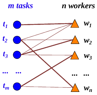
Figure 4: Illustration of the Task-and-Worker Assignment.

5 The Sampling Approach

5.1 Random Sampling Algorithm

In this subsection, we illustrate how to obtain a good task-and-worker assignment strategy with high reliability and diversity by random sampling. Specifically, in our RDB-SC problem, all possible task-and-worker assignments correspond to the population, where each assignment is associated with a value (i.e., reliability or diversity). As shown in Figure 4, we denote $m$ tasks $t_{i}$ and $n$ workers $w_{j}$ by nodes of circle and triangle shapes, respectively. The edge between two types of nodes indicates that worker $w_{j}$ can arrive at the location of task $t_{i}$ within the time period (and with correct moving direction as well). Since each worker can be only assigned to one task, for each worker node $w_{j}$, we can select one of $deg(w_{j})$ edges connecting to it (represented by bold edges in the figure), where $deg(w_{j})$ is the degree of the worker node $w_{j}$. As a result, we can obtain $n$ selected edges (as shown in Figure 4), which correspond to one possible assignment of workers to tasks.

Due to the exponential number ($O(\prod_{j=1}^{n}deg(w_{j}))$) of possible assignments (i.e., large size of the population), it is not feasible to enumerate all assignments, and find an optimal assignment with high reliability and diversity. Alternatively, we adopt the sampling techniques, and aim at obtaining $K$ random samples from the entire population such that among these $K$ samples there exists a sample with error-bounded ranks of reliability or diversity.

Figure 5 illustrates the pseudo code of our sampling algorithm, RDB-SC_Sampling, to tackle the RDB-SC problem. Specifically, we obtain each random sample (i.e., task-and-worker assignment), $S_{h}$ ($1\leq h\leq K$), from the entire population as follows. For each worker $w_{j}$ ($1\leq j\leq n$), we first randomly generate an integer $x$ between $[1,deg(w_{j})]$, and then select the $x$-th edge that connecting two nodes $t_{i}$ and $w_{j}$ (lines 5-7). After selecting $n$ edges for $n$ workers, respectively, we can obtain one possible assignment, which is exactly a random sample $S_{h}$ ($1\leq h\leq K$). Here, the random sample $S_{h}$ is chosen with a probability $p=\prod_{j=1}^{n}\frac{1}{deg(w_{j})}$. Given the sample (assignment) $S_{h}$, we can compute its reliability and diversity.

We repeat the sampling process above, until $K$ samples (i.e., assignments) are obtained. After obtaining $K$ samples, we rank them with the ranking scores [22] (w.r.t. reliability and diversity) (line 8). Let $S_{h}$ be the sample with the highest score (line 9). We can return this sample (assignment) as the answer to the RDB-SC problem (line 10).

Procedure RDB-SC_Sampling { Input: $m$ time-constrained spatial tasks in $T$ and $n$ workers in $W$ Output: a task-and-worker assignment strategy, $\mathbb{S}$,with high reliability and diversity (1) $\mathbb{S}=\emptyset$ (2) compute all the valid task-and-worker pairs $(t_{i},w_{j})$ (3) for $h=1$ to $K$ // in each round, obtain one random sample $S_{h}$ (4) $S_{h}=\emptyset$ (5) for each worker $w_{j}$ ($\in W$) (6) randomly select a task $t_{i}$ with probability $\frac{1}{deg(w_{j})}$ (7) $S_{h}=S_{h}\cup\{(t_{i},w_{j}\}$ (8) rank $S_{h}$ ($1\leq h\leq K$) by dominating scores among samples (9) let $\mathbb{S}$ be the sample, $S_{h}$, with the highest score (10) return $\mathbb{S}$ }

Figure 5: RDB-SC Sampling Algorithm.

Intuitively, when the sample size $K$ is approaching the population size (i.e., $\prod_{j=1}^{n}deg(w_{j})$), we can obtain RDB-SC answers close to the optimal solution. However, since RDB-SC is NP-hard and intractable (as proved in Lemma 3.2), we alternatively aim to find approximate solution via samples with bounded rank errors. Specifically, our target is to determine the sample size $K$ such that the sample with the maximum optimization goal (reliability or diversity) has the rank within the $(\epsilon,\delta)$-error-bound.

5.2 Determination of Sample Size

Without loss of generality, assume that we have the population of size $N$ (i.e., $N=\prod_{j=1}^{n}deg(w_{j})$), $V_{1}$, $V_{2}$, …, and $V_{N}$, which correspond to the reliabilities/diversities of all possible task-and-worker assignments, where $V_{1}\leq V_{2}\leq...\leq V_{N}$. Then, for each value $V_{i}$ ($1\leq i\leq N$), we flip a coin. With probability $p$, we accept value $V_{i}$ as the selected random sample; otherwise (i.e., with probability $(1-p)$), we reject value $V_{i}$, and repeat the same sampling process for the next value (i.e., $V_{i+1}$). This way, we can obtain $K$ samples, denoted as $S_{1}$, $S_{2}$, …, and $S_{K}$, where $S_{1}\leq S_{2}\leq...\leq S_{K}$.

Our goal is to estimate the required minimum number of samples, $\widehat{K}$, such that the rank of the largest sample $S_{K}$ is bounded by $\epsilon N$ in the population (i.e., within $((1-\epsilon)\cdot N,N]$) with probability greater than $\delta$.

Let variable $X$ be the rank of the largest sample, $S_{K}$, in the entire population. We can calculate the probability that $X=r$:

$$Pr\{X=r\} = \dbinom{r-1}{K-1}\cdot p^{K-1}\cdot(1-p)^{r-K}\cdot p\cdot(1-p)^{N-r}$$ (13)

$$= \dbinom{r-1}{K-1}\cdot p^{K}\cdot(1-p)^{N-K}.$$

Intuitively, the first 3 terms above is the probability that $(K-1)$ out of $(r-1)$ values are selected from the population before (smaller than) $S_{K}$ (i.e., $V_{1}\sim V_{r-1}$). The fourth term (i.e., $p$) is the probability that the $r$-th largest value $V_{r}$ ($=S_{K}$) is selected. Finally, the last term is the probability that all the remaining $(N-r)$ values (i.e., $V_{r+1}\sim V_{N}$) are not sampled.

With Eq. (13), the cumulative distribution function of variable $X$ is given by:

$$Pr\{X\leq r\}=\sum_{i=1}^{r}Pr\{X=i\}.$$ (14)

Now our problem is as follows. Given parameters $p$, $\epsilon$, and $\delta$, we want to decide the value of parameter $K$ with high confidence. That is, we have:$Pr\{X>(1-\epsilon)\cdot N\}>\delta.$

By applying the combination theory and Harmonic series, we can rewrite the formula $Pr\{X>(1-\epsilon)\cdot N\}>\delta$, and derive the following formula w.r.t. $K$:

$$K>\frac{p\cdot M\cdot e-1+p}{1-p+e\cdot p},$$ (15)

where $M=(1-\epsilon)\cdot N$, and $e$ is the base of the natural logarithm. Please refer the detailed derivation to Appendix F of the technical report [6].

Since $K\leq M$ holds, and the probability $Pr\{X\leq(1-\epsilon)\cdot N\}$ decreases with the increase of K, we can thus conduct a binary search for $\widehat{K}$ value within $\left(\frac{p\cdot M\cdot e-1+p}{1-p+e\cdot p},M\right]$, such that $\widehat{K}$ is the smallest $K$ value such that $Pr\{X\leq(1-\epsilon)\cdot N\}\leq 1-\delta$, where $p=\prod_{j=1}^{n}\frac{1}{deg(w_{j})}$.

This way, we can first calculate the minimum required sample size, $\widehat{K}$, in order to achieve the $(\epsilon,\delta)$-bound. Then, we apply the sampling algorithm mentioned in Section 5.1 to retrieve samples. Finally, we calculate one sample with the highest reliability and diversity. Note that, in the case no sample dominates all other samples, we select one sample with the highest ranking score (i.e., dominating the most number of other samples) [22].

6 The Divide-and-Conquer Approach

6.1 Divide-and-Conquer Algorithm

We first illustrate the basic idea of the divide-and-conquer approach. As discussed in Section 5.1, the size of all possible task-and-worker assignments is exponential. Although RDB-SC is NP-hard, we still can speed up the process of finding the RDB-SC answers. By utilizing divide-and-conquer approach, the problem space is dramatically reduced.

Figure 6 illustrates the main framework for our divide-and-conquer approach, which includes three stages: (1) recursively divide the RDB-SC problem into two smaller subproblems, (2) solve two subproblems, and (3) merge the answers of two subproblems. In particular, for Stage (1), we design a partitioning algorithm, called BG_Partition, to divide the RDB-SC problem into smaller subproblems. In Stage (2), we use either the greedy or sampling algorithm, introduced in Section 4 and Section 5, respectively, to get an approximation result. Moreover, for Stage (3), we propose an algorithm, called SA_Merge, to obtain RDB-SC answers by combining answers to subproblems.

Procedure RDB-SC_DC { Input: $m$ time-constrained spatial tasks in $T$, $n$ workers in $W$, and a threshold $\gamma$ Output: two sparse and balanced tasks-workers set pairs (1) if $Size(T)\leq\gamma$ (2) solve problem ($T$,$W$) to get the result $\mathbb{S}$ directly (3) else (4) BG_Partition ($T$,$W$) to ($T_{1}$,$W_{1}$) and ($T_{2}$,$W_{2}$) (5) RDB-SC_DC ($T_{1}$,$W_{1}$) to get answer $\mathbb{S}_{1}$ (6) RDB-SC_DC ($T_{2}$,$W_{2}$) to get answer $\mathbb{S}_{2}$ (7) SA_Merge ($\mathbb{S}_{1}$, $\mathbb{S}_{2})$ to get the result $\mathbb{S}$ (8) return $\mathbb{S}$ }

Figure 6: Divide and Conquer Algorithm.

6.2 Partition the Bipartite Graph

As shown in Figure 4, the task-and-worker assignment is a bipartite graph. We first need to iteratively divide the whole graph into two subgraphs such that few edges crossing the cut (sparse) and close to bisection (balanced). Unfortunately, this problem is NP-hard [11]. Here we just provide a heuristic algorithm, namely BG_Partition, which is shown in Figure 7. After running BG_Partition we can get two subproblems $RDB\text{-}SC_{1}$ and $RDB\text{-}SC_{2}$.

Procedure BG_Partition { Input: $m$ time-constrained spatial tasks in $T$ and $n$ workers in $W$ Output: two sparse and balanced tasks-workers set pairs (1) $W_{1}=\varnothing,W_{2}=\varnothing$ (2) partition tasks into two even set $T_{1}$ and $T_{2}$ with KMeans (3) for $w_{i}$ in $W$ (4) if the tasks that $w_{i}$ can do are all included in $T_{1}$ (5) put $w_{i}$ into $W_{1}$ and $W=W-\{w_{i}\}$ (6) if the tasks that $w_{i}$ can do are all included in $T_{2}$ (7) put $w_{i}$ into $W_{2}$ and $W=W-\{w_{i}\}$ (8) add $W$ into $W_{1}$ (9) add $W$ into $W_{2}$ (10) return $(T_{1},W_{1})$ and $(T_{2},W_{2})$ }

Figure 7: Bipartite Graph Partitioning Algorithm.

First, we partition tasks into two almost even subsets, $T_{1}$ and $T_{2}$, based on their locations, which can be done through clustering the tasks to two set (i.e. KMeans.). Then we find out the workers who can reach tasks totally included in some subset, and add them to the corresponding worker subset, $W_{1}$ or $W_{2}$. By doing this, these workers are isolated in the corresponding subproblems. For the rest workers who can do tasks both in $T_{1}$ and $T_{2}$, we add them to both $W_{1}$ and $W_{2}$. As Figure 8 shows, $w_{1}$ and $w_{5}$ are isolated in $RDB\text{-}SC_{1}$ and $RDB\text{-}SC_{2}$ respectively while $w_{2},w_{3},w4$ are added in both two subproblems.

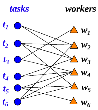
(a) Origin Problem

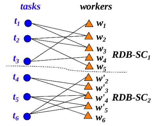
(b) Partitioned Problem

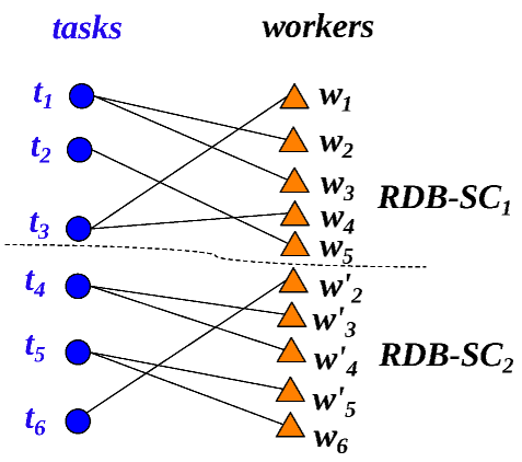
(c) ICW and DCW

Figure 8: Illustration of the Task-and-Worker Partitioning

Note that, even if some workers are duplicated and added to both $W_{1}$ and $W_{2}$, each of them can only be assigned to one task. Moreover, the duplicated workers in each subproblem can only do a part of the tasks that he can do in the whole problem. The complexity of $RDB\text{-}SC_{1}$ or $RDB\text{-}SC_{2}$ are much lower than $RDB\text{-}SC$. Each time before calling BG_Partition algorithm, we check whether the size of the tasks is greater than a threshold $\gamma$, otherwise that problem is small enough to solve directly. The threshold $\gamma$ is set before running the divide-and-conquer algorithm.

6.3 Merge the Answers of the Subproblems

To merge the answers of the subproblems, we just need to solve the conflicts of the workers who are added to both two subproblems. Those duplicated workers in are called conflicting workers, whereas others are called non-conflicting workers. We first give the property of deleting one copy of a conflicting worker.

A conflicting worker $w_{i}$ is called independent conflicting worker (ICW), when $w_{i}$ is assigned to tasks $t_{i1}$ and $t_{i2}$ in the optimal assignments for $RDB\text{-}SC_{1}$ and $RDB\text{-}SC_{2}$, respectively, and no other conflicting workers are assigned to either $t_{i1}$ or $t_{i2}$. Otherwise, $w_{i}$ is called dependent conflicting worker (DCW). For example, in Figure 8(c) worker $w_{5}$ is a ICW and worker $w_{2}$ is a DCW.

Lemma 6.1.

(Non-conflict Stable) The deletion of those conflicting workers’ copies will not change the assignments of non-conflicting workers who are assigned to a same task with any deleted worker.

Proof 6.2.

Please refer to Appendix G of the technical report [6].

Lemma 6.3.

(Deletion of copies of ICWs and DCWs) The deletion of copies of ICWs can be done independently while DCWs’ deletion need to be considered integrally.

Proof 6.4.

Please refer to Appendix H of the technical report [6].

With Lemmas 6.1 and 6.3, the algorithm for merging subproblems is shown in Figure 9, called SA_Merge.

Procedure SA_Merge { Input: two subproblems ($T_{1},W_{1}$) and ($T_{2},W_{2}$), and their local answer $\mathbb{S}_{1}$ and $\mathbb{S}_{2}$ Output: one merged problem’s answer $\mathbb{S}$ for ($T_{1}\cup T_{2},W_{1}\cup W_{2}$) (1) $W^{\prime}=W_{1}\cap W_{2}$ (2) while $W^{\prime}$ is not empty (3) pick first worker in $W^{\prime}$ as $w_{t}$ (4) find out dependent workers for $w_{t}$ as $W_{d}$ (5) add $w_{t}$, $W_{d}$ into $W_{t}$ (6) remove one copy of each worker in $W_{t}$ from $\mathbb{S}_{1}$ and $\mathbb{S}_{2}$ integrally (7) $W^{\prime}=W^{\prime}-W_{t}$ (8) $\mathbb{S}=\mathbb{S}_{1}\cup\mathbb{S}_{2}$ (9) return $\mathbb{S}$ }

Figure 9: Algorithm of Merging Answers to Subproblems.

7 Cost-Model-Based Grid Index

7.1 Index Structure

We first illustrate the index structure, namely RDB-SC-Grid, for the RDB-SC system. Specifically, in a 2-dimensional data space $[0,1]^{2}$, we divide the space into $1/\eta^{2}$ square cells with side length $\eta$, where $\eta<1$ and we discuss in Appendix I of the technical report [6] about how to set $\eta$ based on a cost model.

Each cell has a unique ID, $cellid$, and contains a task list and a worker list which store tasks and workers in it, respectively. In each task list, we maintain quadruples $(tid,l,s,e)$, where $tid$ is the task ID, $l$ is the position of the task, and $[s,e]$ is the valid period of the task. In each worker list, we keep records in the form $(wid,l,v,\alpha^{-},\alpha^{+},p)$, where $wid$ is the worker ID, $l$ and $v$ represent the location and velocity of the worker, respectively, $[\alpha^{-},\alpha^{+}]$ indicates the angle range of moving directions, and $p$ is the reliability of the worker. For each cell, we also maintain bounds, $[v_{min},v_{max}]$, for velocities of all workers in it, $[\alpha_{min},\alpha_{max}]$, for all workers’ moving directions, and $[s_{min},e_{max}]$ of tasks’ time constraints, where $s_{min}$ is the earliest start time of tasks stored in the cell, and $e_{max}$ is the latest deadline in the cell. In addition, each cell is associated with a list, $tcell\_list$, which contains all the IDs of cells that can be reachable to at least one worker in that cell.

Pruning Strategy on the Cell Level. One straightforward way to construct $tcell\_list$ for cell $cell_{i}$ is to check all cells $cell_{j}$, and add those “reachable” cells to $tcell\_list$. This is however quite time-consuming to check each pair of worker and task from $cell_{i}$ and $cell_{j}$, respectively. In order to accelerate the efficiency of building $tcell\_list$, we propose a pruning strategy to reduce the search space. That is, for cell $cell_{i}$, if a cell, $cell_{j}$, is in the reachable area (in workers’ moving directions) within two rays starting from $cell_{i}$ (i.e., reachable by at least one worker in $cell_{i}$), then we add $cell_{j}$ to list $tcell\_list$ of $cell_{i}$. Therefore, our pruning strategy can effectively filter out those cells that are definitely unreachable.

Specifically, we can prune $cell_{j}$ as follows. First, we calculate the minimum and maximum distances, $d_{min}$ and $d_{max}$, respectively, between any two points in $cell_{i}$ and $cell_{j}$. As a result, any worker who moves from $cell_{i}$ will arrive at $cell_{j}$ with time at least $t_{min}=\frac{d_{min}}{v_{max}(cell_{i})}$, where $v_{max}(cell_{i})$ is the maximum speed in $cell_{i}$. Thus, if $t_{min}>e_{max}(cell_{i})$, we can safely prune $cell_{j}$, where $e_{max}(cell_{i})$ represents the latest deadline of tasks in $cell_{i}$. After pruning these unreachable cells, we further check the rest cells one by one to build the final $tcell\_list$ for $cell_{i}$.

Please refer to Appendix I of the technical report [6].

7.2 Dynamic Maintenance

To insert a worker $w_{i}$ into RDB-SC-Grid, we first find the cell $cell_{k}$ where $w_{i}$ locates, which uses $O(1)$ time. Moreover, we also need to update the $tcell\_list$ for $cell_{k}$, which requires $O(cost_{update})$ time in the worst case. The case of removing a worker is similar.

To insert a task $t_{j}$ into RDB-SC-Grid, we obtain the cell, $cell_{k}$, for the insertion, which requires $O(1)$ time cost. Furthermore, we need to check all the cells that do not contain $cell_{k}$ in their $tcell\_list$’s, which needs to check all workers in the worst case (i.e., $O(n)$). When removing a task from $cell_{k}$, we check all the cells containing it in their $tcell\_list$s, which also requires to check every worker in the worst case (i.e., $O(n)$).

8 Experimental Study

8.1 Experimental Methodology

Table 2: Experiments setting.

Parameter	Values
range of expiration time $rt$	[0.25, 0.5], [0.5, 1], [1, 2], [2, 3]
reliability of workers $[p_{min},p_{max}]$	(0.8, 1), (0.85, 1), (0.9, 1), (0.95, 1)
number of tasks $m$	5K, 8K, 10K, 50K, 100K
number of workers $n$	5K, 8K, 10K, 15K, 20K
velocities of workers $[v^{-},v^{+}]$	[0.1, 0.2],[0.2, 0.3], [0.3, 0.4], [0.4, 0.5]
range of moving angles ($\alpha_{j}^{+}-\alpha_{j}^{-}$)	(0, $\pi$/8], (0, $\pi$/7], (0, $\pi$/6], (0, $\pi$/5], (0, $\pi$/4]
balancing weight $\beta$	(0, 0.2], (0.2, 0.4], (0.4, 0.6], (0.6, 0.8], (0.8, 1)

Data Sets. We use both real and synthetic data to test our approaches. Specifically, for real data, we use the POI (Point of Interest) data set of China [9] and T-Drive data set [23, 24]. The POI data set of China contains over 6 million POIs of China in 2008, whereas T-Drive data set includes GPS trajectories of 10,357 taxis within Beijing during the period from Feb. 2 to Feb. 8, 2008. We test our approaches in the area of Beijing (with latitude from $39.6\mathrm{°}$ to $40.25\mathrm{°}$ and longitude from $116.1\mathrm{°}$ to $116.75\mathrm{°}$), which covers 74,013 POIs. After filtering out short trajectories from T-Drive data set, we obtain 9,748 taxis’ trajectories. We use POIs to initialize the locations of tasks. From the trajectories, we extract workers’ locations, ranges of moving directions, and moving speeds. For workers’ confidences $p$, tasks’ valid periods $[s,e]$, and parameter $\beta$ to balance spatial and temporal diversity, we follow the same settings as that in synthetic data (as described below).

For synthetic data, we generate locations of workers and tasks in a 2D data space $[0,1]^{2}$, following either Uniform (UNIFORM) or Skewed (SKEWED) distribution. In particular, similar to [18], we generate tasks and workers with Skewed distribution by letting 90% of tasks and workers falling into a Gaussian cluster (centered at (0.5, 0.5) with variance = $0.2^{2}$). For each moving worker $w_{j}$, we randomly produce the angle range, $[\alpha_{j}^{-},\alpha_{j}^{+}]$, where $\alpha_{j}^{-}$ is uniformly chosen within $[0,2\pi]$ and $(\alpha_{j}^{+}-\alpha_{j}^{-})$ is uniformly distributed in a range of angle (e.g., $(0,\pi/6]$). Moreover, we also generate check-in times of each worker with Uniform or Skewed distribution, and compute one’s confidence (reliability) following Gaussian distribution within the range $[p_{min},p_{max}]$ (with mean $\frac{p_{min}+p_{max}}{2}$, and variance $0.02^{2}$). Furthermore, we obtain the velocity of each worker with either Uniform or Gaussian distribution within range $[v^{-},v^{+}]$, where $v^{-},v^{+}\in(0,1)$. Regarding spatial tasks, we generate their valid periods, $[s,e]$, within a time interval $[st,st+rt]$, where $st\in[0,24]$ follows either Uniform or Gaussian distribution, and $rt$ follows the Uniform distribution. To balance $SD$ and $TD$, we test parameter $\beta$ following Uniform distribution within $[0,1]$. The case of $rt$ or $\beta$ following other distributions is similar, and thus omitted due to space limitations.

Configurations of a Customized gMission Spatial Crowdsourcing Platform. We tested the performance of our proposed algorithms with an incrementally updating strategy, on a real spatial crowdsourcing platform, namely gMission [7, 15]. In particular, gMission is a general laboratory application, which has over 20 existing active users in the Hong Kong University of Science and Technology. In gMission, users can ask/answer spatial crowdsourcing questions (tasks), and the platform pushes tasks to users based on their spatial locations. As gMission has been released, the recruitment, monitoring and compensation of workers are already provided. A credit point system of gMission can record the contribution of workers. Workers can use their credit point to redeem coupons of book stores or coffee shops. Moreover, when they are using gMission, their trajectories are recorded, which is informed to the users. To evaluate our RDB-SC model and algorithms, we will modify/adapt gMission to an RDB-SC system.

Specifically, in order to build user profiles, we set up the peer-rating over 613 photos taken by active users. They are asked to rate peers’ photos based on their resolutions, distances, and lights. The score of each photo is given by first removing the highest and lowest scores, and then averaging the rest. Moreover, the score of each user is given by the average score of all photos taken by this user. Intuitively, a user receiving a higher score is more reliable. Thus, we set the user’s peer-rating score as one’s reliability value.

In addition, we also provide a setting option for users to configure their preferred working area. For example, a user is going home, and wants to do some tasks on the way home. In general, one may just want to go to places not deviating from the direction towards his/her home too much. Thus, a fan-shaped working area is reasonable. Due to the maximum possible speed of the user, this fan-shaped working area is also constrained by the maximum moving distance.

Furthermore, we enable gMission to detect the accuracy of answers. When a worker $w_{j}$ is taking a photo to answer a task $t_{i}$, we record his/her instantaneous information, like the facing direction, the location, and the timestamp, through his/her smart device. By comparing the information with the required angle and time constraint of $t_{i}$, we can calculate the error of angle $\Delta\theta_{ij}$ and the error of time $\Delta t_{ij}$. Then, the accuracy of the answer is $Accuracy_{ij}=\beta_{i}\cdot\frac{\Delta\theta_{ij}}{\pi}+(1-\beta_{i})\cdot\frac{\Delta t_{ij}}{e_{i}-s_{i}}$, where $\beta_{i}$ is the balancing weight of $t_{i}$, and $s_{i}$ and $e_{i}$ are the starting and ending times, respectively. In particular, $0\leq\Delta\theta_{ij}\leq\pi$ and $0\leq\Delta t_{ij}<e_{i}-s_{i}$. Then, the accuracy of a task is given by the average value of all accuracy values of the answers to the task. For the accuracy control, it could be quite interesting and challenging, and we would like to leave it as our future work.

In order to deploy our proposed algorithms, we implement the cost-model-based grid index, and apply the incremental updating strategy for dynamically-changing tasks and workers to our RDB-SC system. The framework for the incremental updating strategy is shown in Figure 10 below. In line 6 of the framework (Figure 10), we can use our proposed algorithms to assign the available workers to the opening tasks, where considering $A$ and $\mathbb{S}_{c}$ means the reliability and diversity of a task $t_{i}$ is calculated from the received answers, the workers assigned to $t_{i}$ in $\mathbb{S}_{c}$, and newly assigned workers. In particular, we periodically update the task-and-worker assignments every $t_{interval}$ timestamps. For each update, those workers, who either have accomplished the assigned tasks or rejected the assignment requests, would be available to receive new tasks. In our experiments, we set this length, $t_{interval}$, of the periodic update interval, from 1 minute to 4 minutes, with an increment of 1 minute. We hired 10 active users in our experiments and chose 5 sites to ask spatial crowdsourcing questions (tasks) with 15 minutes opening time. The sites are close to each other, and in general a user can walk from one site to another one within 2 minutes.

Procedure RDB-SC_Incremental { Input: $m$ time-constrained spatial tasks in $T$, $n$ workers in $W$, Output: a updated task-and-worker assignment strategy, $\mathbb{S}$, with high reliability and diversity (1) $\mathbb{S}=\emptyset$ (2) from $W$, retrieve all the available workers to $W_{a}$ (3) from $T$, retrieve all the opening tasks to $T_{a}$ (4) obtain the received answers of all the tasks in $W_{a}$, noted as $A$ (5) obtain the current assignment, noted as $S_{c}$ (6) assign workers in $W_{a}$ to tasks in $T_{a}$ considering $A$ and $S_{c}$ (new pairs are added to $\mathbb{S}$ ) (7) $\mathbb{S}=\mathbb{S}\cup\mathbb{S}_{c}$ (8) return $\mathbb{S}$ }

Figure 10: Incremental Updating Strategy.

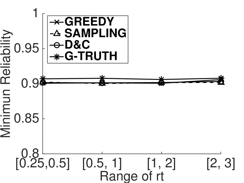
(a) Minimum Reliability

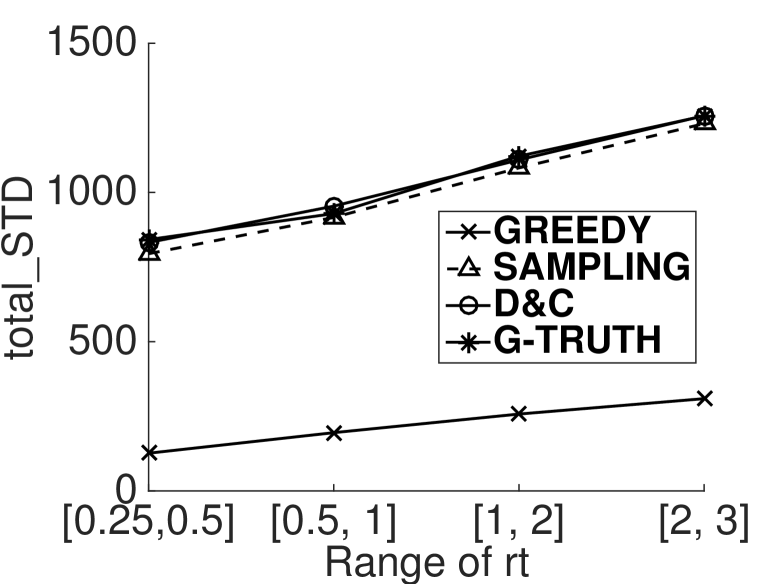
(b) Summation of Diversity

Figure 11: Effect of Tasks’ Expiration Time Range of $rt$

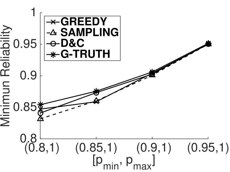
(a) Minimum Reliability

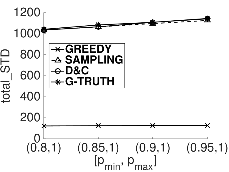
(b) Summation of Diversity

Figure 12: Effect of Workers’ Reliability $[p_{min},p_{max}]$

RDB-SC Approaches and Measures. Greedy (GREEDY) assigns each worker to a “best” task according to the current situation when processing the worker, which is just a local optimal approach. Sampling (SAMPLING) randomly assigns all the available workers several times and picks the best test result, using our equations in Section 5.2 to calculate the sampling times to bound the accuracy. Divide-and-Conquer (D&C) divides the original problem into subproblems, solves each one and merges their results. To accelerate D&C, we use SAMPLING to solve subproblems of D&C, which will sacrifice a little accuracy. Nonetheless, this trade-off is effective, we will show SAMPLING has a good performance when the problem space is small in our experiments. To evaluate our 3 proposed approaches, we will compare them with the ground truth. However, since RDB-SC problem is NP-hard (as discussed in Section 3.2), it is infeasible to calculate the real optimal result as the ground truth. Thus, we use Divide-and-Conquer approach with the embedded sampling approach (discussed in Section 5) to calculate sub-optimal result by setting the sampling size 10 times larger than D&C (denoted as G-TRUTH).

Table 2 depicts the experimental settings, where the default values of parameters are in bold font. In each set of experiments, we vary one parameter, while setting others to their default values. We report $\min_{i=1}^{m}rel(t_{i},W_{i})$, the minimum reliability, and $total\_STD$, the summation of the expected spatial/temporal diversities. All our experiments were run on an Intel Xeon X5675 CPU @3.07 GHZ with 32 GB RAM.

8.2 Experiments on Real Data

In this subsection, we show the effects of workers’ confidence $p$, tasks’ valid periods $[s,e]$ and balancing parameter $\beta$ on the real data. We use the locations of the POIs as the locations of tasks. To initialize a worker based on trajectory records of a taxi, we use the start point of the trajectory as the worker’s location, use the average speed of the taxi as the worker’s speed. For the moving angle’s range of the worker, we draw a sector at the start point and contain all the other points of the trajectory in the sector, then we use the sector as the moving angle’s range of the worker. We uniformly sample 10,000 POIs from the 74,013 POIs in the area of Beijing and the sampled POI date set follows the original data set’s distribution. In other words, we have 10,000 tasks and 9,748 workers in the experiments on real data.

Effect of the Range of Tasks’ Expiration Times $rt$. Figure 11 shows the effect of varying the range of tasks’ expiration times $rt$. When this range increases from $[0.25,0.5]$ to $[2,3]$, the minimum reliability is very stable, and the diversities $total\_STD$ of all the approaches gradually increase. Intuitively, longer expiration time for a task $t_{i}$ means more workers can arrive at location $l_{i}$ to accomplish $t_{i}$. From the perspective of workers, each worker can have more choices in his/her reachable area. Thus, each worker can choose a better target task with higher diversity. Similar to previous results, SAMPLING and D&C approaches can achieve higher diversities than GREEDY, and slightly lower diversities compared with G-TRUTH. The requester can use this parameter to constrain the range of the opening time of a task. For example, if one wants to know the situation of a car park in a morning, he/she can set the time range as the period of the morning.

Effect of the Range of Workers’ Reliabilities $[p_{min},p_{max}]$. Figure 12 reports the effect of the range, $[p_{min},p_{max}]$, of workers’ reliabilities on the reliability/diversity of our proposed RDB-SC approaches. For the minimum reliability, the reliabilities of workers may greatly affect the reliability of spatial tasks (as given by Eq. (1)). Thus, as shown in Figure 12(a), for the range with higher reliabilities, the minimum reliability of tasks also becomes larger. For diversity $total\_STD$, according to Lemma 3.1, when the workers assigned to tasks $t_{i}$ have higher reliabilities, the expected spatial/temporal diversity will be higher. Therefore, we can see the slight increases of $total\_STD$ in Figure 12(b). Similar to previous results, SAMPLING and D&C show reliability and diversity similar to G-TRUTH, and have higher diversities than GREEDY.

We test the effect of the requester-specified weight range. Due to space limitations, please refer to the experimental results with different $\beta$ values in Appendix J of the technical report [6]. Requesters can use this parameter to reflect their preference. The valid value of $\beta$ is from 0 to 1. The bigger $\beta$ is, the more spatial diverse the answers are. The smaller $\beta$ is, the more temporal diverse the answers are. If one has no preference, he/she can simply set $\beta$ to 0.5.

8.3 Experiments on Synthetic Data

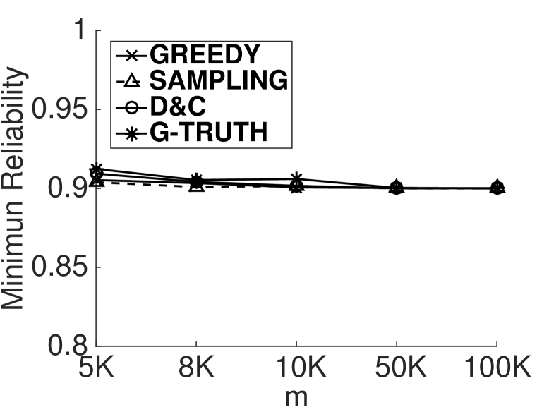
(a) Minimum Reliability

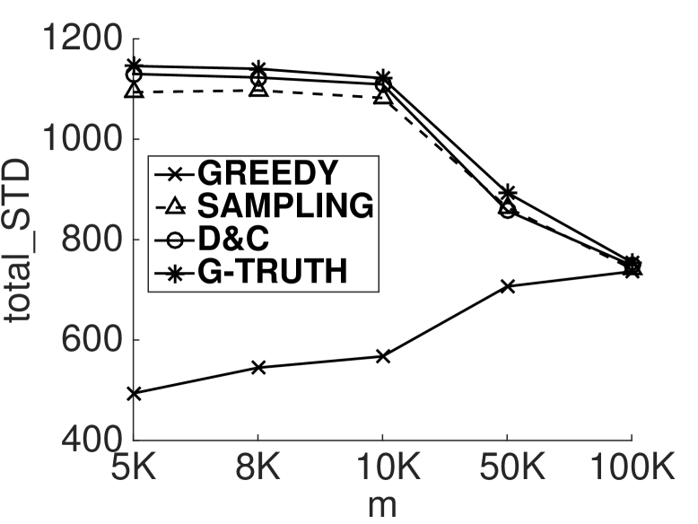
(b) Summation of Diversity

Figure 13: Effect of the Number of Tasks $m$ (UNIFORM)

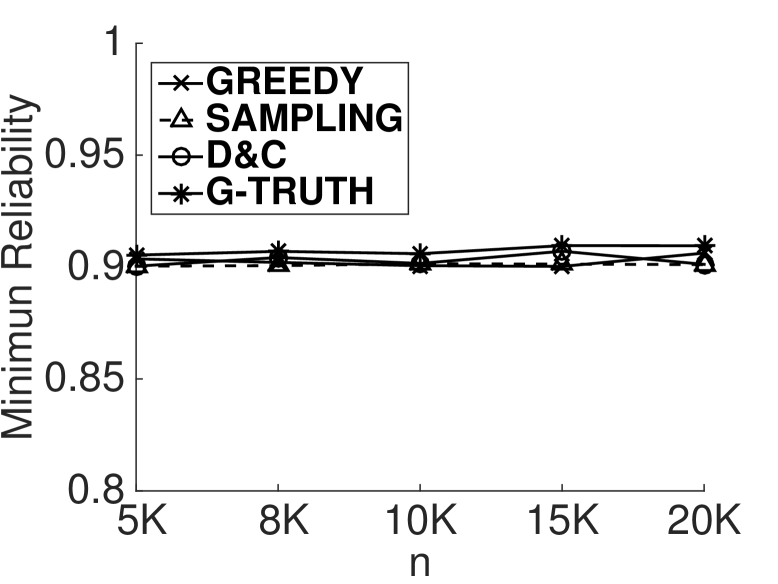
(a) Minimum Reliability

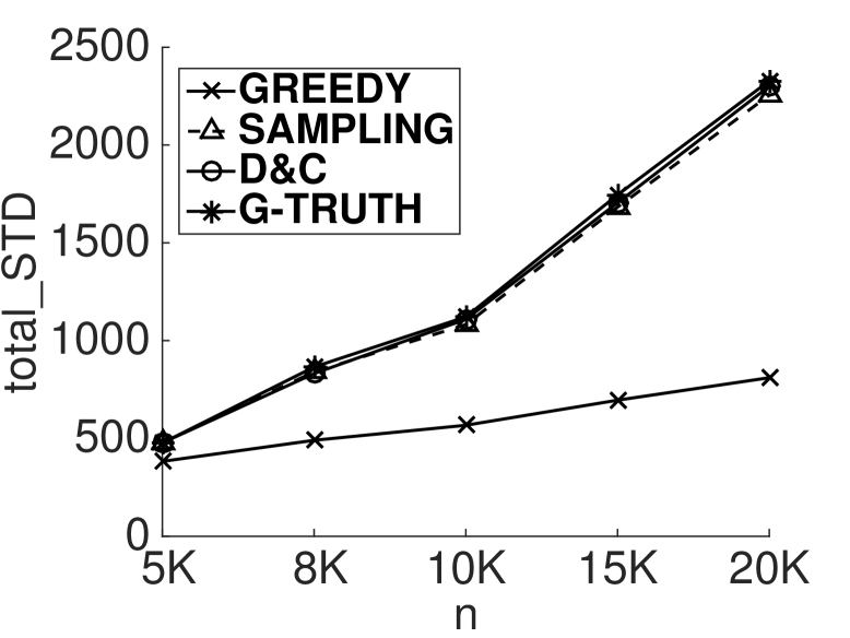
(b) Summation of Diversity

Figure 14: Effect of the Number of Workers $n$ (UNIFORM)

In this subsection, we test the effectiveness and robustness of our proposed 3 RDB-SC approaches, GREEDY, SAMPLING, and D&C, compared with G-TRUTH, by varying different parameters.

As we already see the effects of $p$ and $[s,e]$, we will focus on the rest four parameters in Table 2 in this subsection. We first report the experimental results on Uniform task/worker distributions. Please refer to more (similar) experimental results over data sets with Uniform/Skew distributions in Appendix J of the technical report [6].

Effect of the Number of Tasks $m$. Figure 13 shows the effect of the number, $m$, of spatial tasks on the reliability and diversity of RDB-SC answers, where we vary $m$ from 5K to 100K. In Figure 13(a), all the 3 approximation approaches can achieve good minimum reliability, which are close to G-TRUTH, and remain high (i.e., with reliability around 0.9). The reliability of D&C is higher than that of the other two approaches. When the number, $m$, of tasks increases, the minimum reliability slightly decreases. This is because given a fixed (default) number of workers, our assignment approaches trade a bit the reliability for more accomplished tasks.

For the diversity, our 3 approaches have different trends for larger $m$. In Figure 13(b), for large $m$, the total diversity, $total\_STD$, of GREEDY becomes larger, while that of the other two approaches decreases. For GREEDY, more tasks means more possible task targets for each worker on average. This can make a particular worker to choose one possible task such that high diversity is obtained. In contrast, for SAMPLING, when the number of tasks increases, the size of possible combinations increases dramatically. Thus, under the same accuracy setting, the result will be relatively worse (as discussed in Section 5.2). In D&C, we divide the original problem into several subproblems of smaller scale. Since the number of possible combinations in subproblems decreases quickly, we can achieve good solutions to subproblems. After merging answers to subproblems, D&C can obtain a slightly higher $total\_STD$ than SAMPLING (about 3% improvement). We can see that, both SAMPLING and D&C have $total\_STD$ very close to G-TRUTH, which indicates the effectiveness of SAMPLING and D&C.

In Figure 13(b), when $m$ is small, SAMPLING and D&C can achieve much higher $total\_STD$ than that of GREEDY. The reason is that GREEDY has a bad start-up performance. That is, when most reachable tasks of a worker are not assigned with workers (namely, empty tasks), he/she is prone to join those tasks that already have workers. In particular, when a worker joins an empty task, he/she can only improve the temporal diversity (TD) of that task, and has no contribution to the spatial diversity (SD), according to the definitions in Section 2.3. On the other hand, if a worker joins a task that has already been assigned with some workers, then his/her join can improve both SD and TD, which leads to higher STD. Since GREEDY always chooses task-and-worker pairs that increase the diversity most, GREEDY will always exploit those non-empty tasks, which may potentially miss the good assignment with high diversity $total\_STD$. Thus, $total\_STD$ of GREEDY is low when $m$ is 5K - 10K.

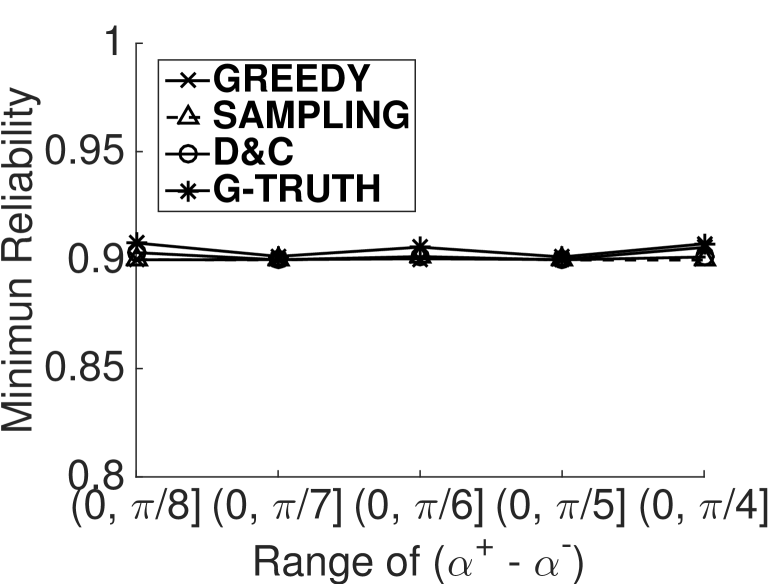
(a) Minimum Reliability

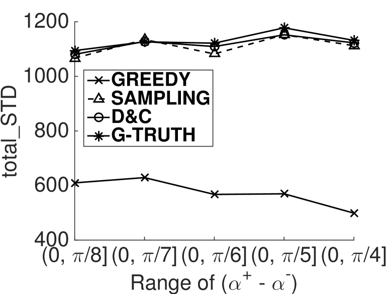
(b) Summation of Diversity

Figure 15: Effect of the Range of Angles $(\alpha_{j}^{+}-\alpha_{j}^{-})$(UNIFORM)

Effect of the Number of Workers $n$. Figure 14 illustrates the experimental results on different numbers, $n$, of workers from $5K$ to $20K$. In Figure 14(a), the minimum reliability is not very sensitive to $n$. This is because, although we have more workers, there always exist tasks that are assigned with just one worker. According to Eq. (1), the minimum reliability among tasks is very close to the lower bound of workers’ confidences. Thus, the reliability slightly changes with respect to $n$.

On the other hand, the diversities, $total\_STD$, of all the four approaches increase for larger $n$ value. In particular, as depicted in Figure 14(b), the diversity of SAMPLING increases more rapidly than that of GREEDY. Recall from Lemma 4.3 that, more workers means a higher diversity for each task. When the number of workers increases, the average number of workers of each task also increases, which leads to a higher $total\_STD$. Similar to previous results, SAMPLING and D&C have diversities very close to G-TRUTH, which confirms the effectiveness of our approaches.

Effect of the Range of Moving Angles $(\alpha_{j}^{+}-\alpha_{j}^{-})$. Figure 15 varies the range, $(\alpha_{j}^{+}-\alpha_{j}^{-})$, of moving angles for workers $w_{j}$ from $(0,\pi/8]$ to $(0,\pi/4]$. From figures, we can see that the minimum reliability is not very sensitive to this angle range. With different angle ranges, the reliability of our proposed approaches remains high (i.e., above 0.9). Moreover, both SAMPLING and D&C approaches can achieve much higher diversities than GREEDY, and they have diversities similar to G-TRUTH, which indicates good effectiveness against different angle ranges of moving directions. On the other hand, $total\_STD$ of GREEDY drops when angle becomes larger. The reason is similar to the cause of GREEDY’s bad start-up, which is discussed when we show the effect of the number of tasks. Larger angle range means more reachable tasks, then workers are more likely to find a task that has been assigned with workers and join that task, which leads to low diversity. On a real platform, the workers may set this parameter based on their personal interests. For example, if a worker would like to deviate more from his/her moving direction, he/she can set the range of his/her moving angle wider.

We test the effect of the range of workers’ velocities. Due to space limitations, please refer to the experimental results with different ranges, $[v^{-},v^{+}]$, in Appendix J of the technical report [6].

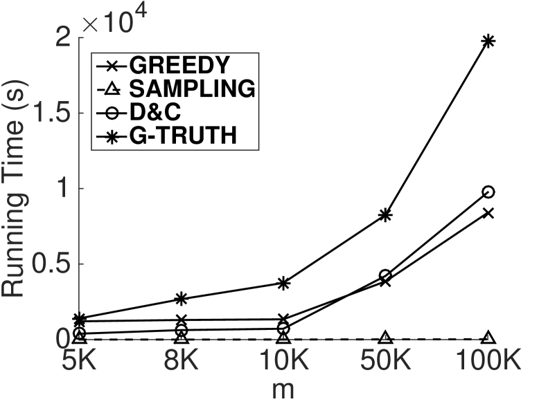
(a) CPU Time (vs. $m$)

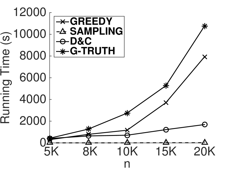
(b) CPU Time (vs. $n$)

Figure 16: Comparisons of the CPU Time with RDB-SC Approaches

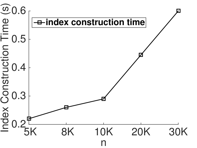
(a) Index Construction Time

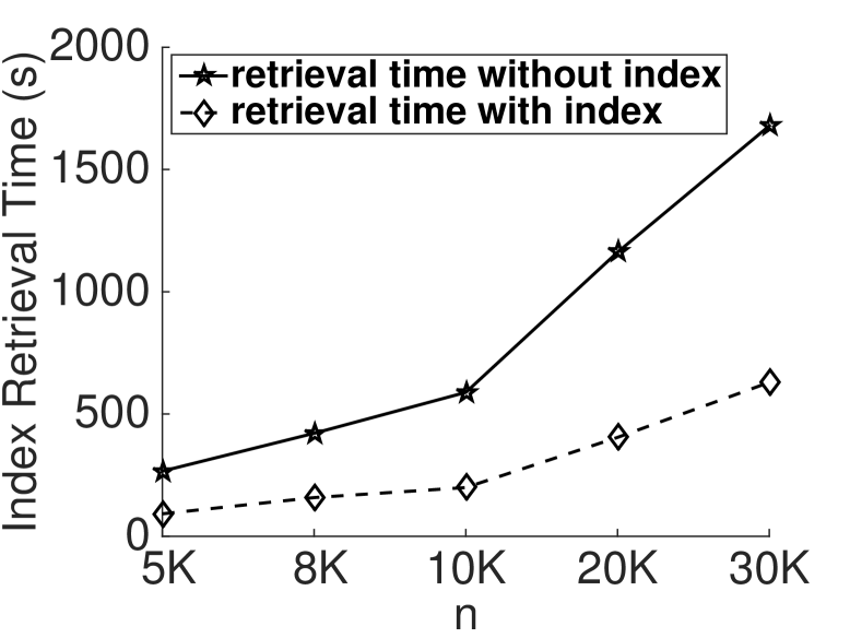
(b) W-T Pairs Retrieval Time

Figure 17: Efficiency of the RDB-SC-Grid Index

Running Time Comparisons and Efficiency of RDB-SC-Grid. We report the running time of our approaches by varying $m$ and $n$ in Figures 16(a) and 16(b), respectively. We can see that, when $m$ increases, the running times of all approaches, except for SAMPLING, grow quickly. For GREEDY, when $m$ increases, each worker has more reachable tasks, and thus the total running time grows (since more tasks should be checked). For large $m$, D&C needs to run more rounds for the divide-and-conquer process, which leads to higher running time. On the other hand, when $n$ increases, only GREEDY’s running time grows dramatically. This is because GREEDY needs to run more rounds to assign workers. Under both situations, SAMPLING only takes several seconds (due to small sample size). In contrast, D&C has higher CPU cost than SAMPLING, however, higher reliability and diversity (as confirmed by Figures 13 and 14). This indicates that D&C can trade the efficiency for effectiveness (i.e., reliability and diversity).

Figure 17 presents the index construction time and index retrieval time (i.e., the time cost for retrieving task-and-worker pairs, denoted as W-T pairs, from the index) over UNIFORM data, where $m=10K$ and $n$ varies from $5K$ to $30K$. As shown in Figure 17(a), the construction time of the RDB-SC-Grid index is small (i.e., less than 0.7 sec). In Figure 17(b), the RDB-SC-Grid index can dramatically reduce the time of finding W-T pairs (up to 67 %), compared with that of retrieving W-T pairs without index.

8.4 Experiments on Real RDB-SC Platform

Figure 18 shows the RDB-SC performance of GREEDY, SAMPLING, D&C, and G-TRUTH over the real RDB-SC system, where the length of the time interval, $t_{interval}$, between every two consecutive incremental updates varies from 1 minute to 4 minutes. In Figure 18(a), when $t_{interval}$ becomes larger, the minimum reliability remains high, except for GREEDY. This is because when $t_{interval}$ is larger than 1 minute, GREEDY assigns just one worker to some tasks, and it leads to sensitive change of the minimum reliability which is much more than that of other algorithms. Each user is assigned with fewer tasks in the entire testing period, when $t_{interval}$ increases. At the same time, GREEDY is prone to assign workers to those tasks already have workers or are answered, which has been discussed when we show the effect of the number of tasks in Section 8.3. When each user is assigned with fewer tasks in the entire testing period, it is more likely to assign only one worker to some task whose reliability will equal to the reliability of that worker. Thus, the minimum reliability of GREEDY varies much.

In Figure 18(b), we can see that for all the approaches, when $t_{interval}$ increases, the total spatial/temporal diversity $total\_STD$ decreases. This is reasonable, since each user is assigned with fewer tasks in the entire testing period. Meanwhile, SAMPLING and D&C are much better than GREEDY from the perspective of the diversity, and their diversities are close to that of G-TRUTH, which indicates the effectiveness of our RDB-SC approaches.

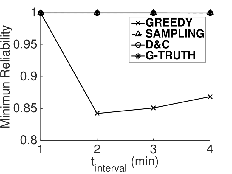
(a) Minimum Reliability

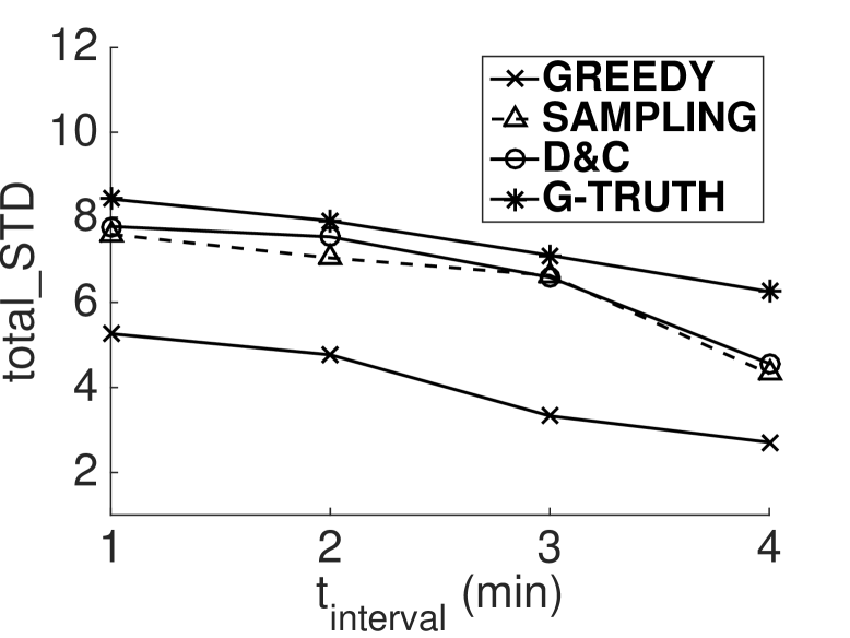
(b) Summation of Diversity

Figure 18: Effect of the updating time interval $t_{interval}$

To show the potential value of our model, we present a 3D reconstruction showcase on gMission’s homepage [7]. We use VisualSFM to build 3D models from unordered photos. As shown in Figure 19, the triangles are the cameras, and their sizes represent the resolutions of those photos. We can see, our approaches can assign workers to the task with a good spatial diversity. Figure 20 compares our final model from the side direction with that of the ground truth. Though we just received 23 photos of the garden in the experiments, the 3D model reconstructed from our test can present a general shape of the garden, as shown in Figure 20(a). The showcase video can be found on Youtube [8].

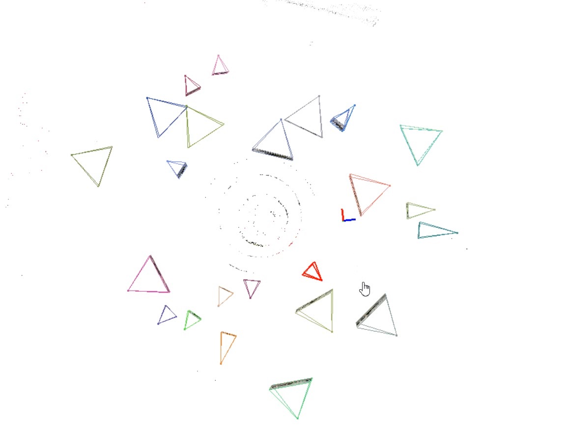
(a) Experiemental Sparse Model

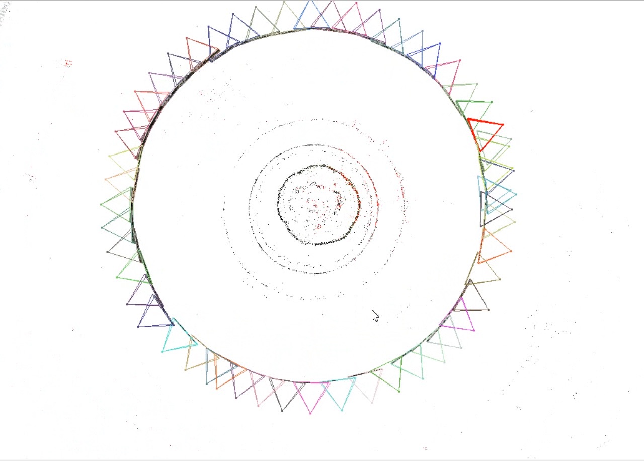
(b) Ground Truth Sparse Model

Figure 19: Comparison of Sparse Models of 3D Reconstruction

(a) Experimental Dense Model

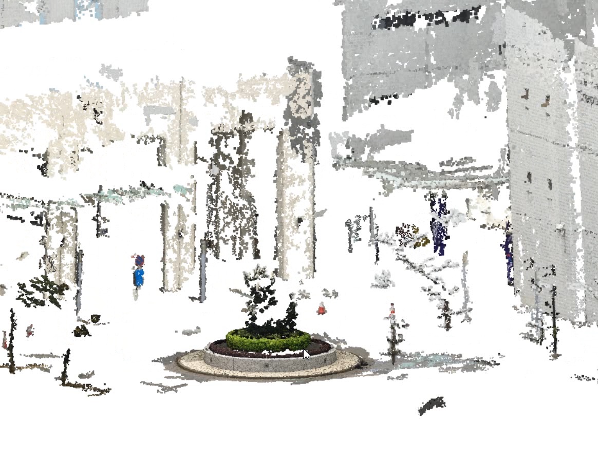
(b) Ground Truth Dense Model

Figure 20: Comparison of Dense Models of 3D Reconstruction

9 Related Work

Recently, with rapid development of GPS-equipped mobile devices, the spatial crowdsourcing [18, 20] that sends location-based requests to workers (based on their spatial positions) has become increasingly important in real applications, such as monitoring real-world scenes (e.g., street view of Google Maps [1]), local hotspots (e.g., Foursquare [3]), and the traffic (e.g., Waze [4]).

Some prior works [10, 14] studied the crowdsourcing problems which treat location information as the parameter, and distribute tasks to workers. However, in these works, workers do not have to visit spatial locations physically (in person) to complete the assigned tasks. In contrast, the spatial crowdsourcing usually needs to employ workers to conduct tasks (e.g., sensing jobs) by physically going to some specific positions. For example, some previous works [16, 19] studied the single-campaign or small-scale participatory sensing problems, which focus on particular applications of the participatory sensing.

According to people’s motivation, Kazemi and Shahabi [20] classified the spatial crowdsourcing into two categories: reward-based and self-incentivised. That is, in the reward-based spatial crowdsourcing, workers can receive a small reward after completing a spatial task; oppositely, for the self-incentivised one, workers perform the tasks voluntarily (e.g., participatory sensing). In this paper, we consider the self-incentivised spatial crowdsourcing.

Furthermore, based on publishing modes of spatial tasks, the spatial crowdsourcing problems can be partitioned into another two classes: worker selected tasks (WST) and server assigned tasks (SAT) [20]. In particular, WST publishes spatial tasks on the server side, and workers can choose any tasks without contacting with the server; SAT collects location information of all workers to the server, and directly assigns workers with tasks. For example, in the WST mode, some existing works [10, 18] allowed users to browse and accept available spatial tasks. On the other hand, in the SAT mode, previous works [19, 20] assumed that the server decides how to assign spatial tasks to workers and their solutions only consider simple metrics such as maximizing the number of assigned tasks on the server side and maximizing the number of worker’s self-selected tasks. In this paper, we not only consider the SAT mode, but also take into account constrained features of workers/tasks (e.g., moving directions of workers and valid period of tasks), which make our problem more complex and unsuitable for borrowing existing techniques.

Kazemi and Shahabi [20] studied the spatial crowdsourcing with the goal of static maximum task assignment, and proposed several heuristics approaches to enable fast assignment of workers to tasks. Similarly, Deng et al. [18] tackled the problem of scheduling spatial tasks for a single worker such that the number of completed tasks by this worker is maximized. In contrast, our work has a different goal of maximizing the reliability and spatial/temporal diversity that spatial tasks are accomplished. As mentioned in Section 1, the reliability and diversity of spatial tasks are very important criteria in applications like taking photos or checking whether or not parking spaces are available. Moreover, while prior works often consider static assignment, our work considers dynamic updates of spatial tasks and moving workers, and proposes a cost-model-based index. Therefore, previous techniques [18, 20] cannot be directly applied to our RDB-SC problem.

Another important topic about the spatial crowdsourcing is the privacy preserving. This is because workers need to report their locations to the server, which thus may potentially release some sensitive location/trajectory data. Some previous works [16, 19] investigate how to tackle the privacy preserving problem in spatial crowdsourcing, which is however out of the scope of this paper.

10 Conclusion

In this paper, we propose the problem of reliable diversity-based spatial crowdsourcing (RDB-SC), which assigns time-constrained spatial tasks to dynamically moving workers, such that tasks can be accomplished with high reliability and spatial/temporal diversity. We prove that the processing of the RDB-SC problem is NP-hard, and thus we propose three approximation algorithms (i.e., greedy, sampling, and divide-and-conquer). We also design a cost-model-based index to facilitate worker-task maintenance and RDB-SC answering. Extensive experiments have been conducted to confirm the efficiency and effectiveness of our proposed RDB-SC approaches on both real and synthetic data sets.

11 acknowledgment

This work is supported in part by the Hong Kong RGC Project N_HKUST637/13; National Grand Fundamental Research 973 Program of China under Grant 2014CB340303; NSFC under Grant No. 61328202, 61325013, 61190112, 61373175, and 61402359; and Microsoft Research Asia Gift Grant.

Appendix

A. Proof of Lemma 3.1.

Proof 11.1.

A spatial diversity entry $M_{SD}[j][k]$ represents the summation of the related elements from all the possible worlds containing angle $A_{j,k}$. In each $pw(W_{i})$ of those possible worlds, the related element is $-(\frac{A_{j,k}}{2\pi})\cdot log(\frac{A_{j,k}}{2\pi})\cdot\prod_{w_{x}\in pw(W_{i})}p_{x}\cdot\prod_{w_{y}\notin pw(W_{i})}(1-p_{y})$. It is easy to find that when we sum up all the related elements, the summation is equal to $M_{SD}[j][k]$. $E(SD(t_{i}))$ is the summation of the diversities of all the possible worlds multiply their probabilities respectively. At the same time, all the possible angles will be taken into consideration when we calculate $E(SD(t_{i}))$. Thus, after combining all the related elements for every angle, we get $E(SD(t_{i}))=\sum_{\forall j,k}M_{SD}[j][k]$. Similarly, we can prove that $E(TD(t_{i}))=\sum_{\forall j,k}M_{TD}[j][k]$.

B. Proof of Lemma 3.2.

Proof 11.2.

We prove the lemma by a reduction from the number partition problem. A number partition problem can be described as follows: Given a set $A=\{a_{1},a_{2},...,a_{N}\}$ of positive integers, find a partitioning strategy, i.e., $A_{1}\subset A$ and $A_{2}=A-A_{1}$, such that the discrepancy $E(A)=\left\lvert\sum_{i\in A_{1}}a_{i}-\sum_{j\in A_{2}}a_{j}\right\rvert$ is minimized. For this given number partition problem, we construct an instance of RDB-SC as follows: first, we give 2 tasks and $n$ workers (each assigned to one of these 2 tasks), and let all the workers and tasks be on the same line, as Figure 21. shows. Moreover, let the beginning times of the 2 tasks is late enough such that every worker can arrive at any task before its expiration time. Under this setting, no matter how to assign the workers, the $total\_STD$ is always zero.

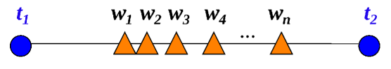
Figure 21: Illustration of the Task-and-Worker Locations.

Next, we set the reliability of the workers based on $A$. Let $a_{max}=\max(A)$ and $a_{i}^{\prime}=a_{i}/a_{max}$. Then, let $p_{i}=1-e^{a_{i}^{\prime}}$.

We now show that we can reduce the number partition problem to our RDB-SC problem. In other words, the result of the number partition problem is also the answer to our designed RDB-SC instance. The answer of this RDB-SC is:

$$\text{maximize }\min(\sum_{w_{i}\in W_{1}}-\ln(1-p_{i}),\sum_{w_{j}\in W_{2}}-\ln(1-p_{j}))$$

$$\implies \text{minimize }\max(\sum_{w_{i}\in W_{1}}\ln(1-p_{i}),\sum_{w_{j}\in W_{2}}\ln(1-p_{j}))$$

$$\implies \text{minimize }\max(\sum_{w_{i}\in W_{1}}a_{i}^{\prime},\sum_{w_{j}\in W_{2}}a_{j}^{\prime})$$

As $\sum_{a_{i}\in A}a_{i}/a_{max}$ is a constant, to minimize the bigger subset sum is same as minimizing the discrepancy to the two subsets, which is the objective of the number partition problem. Given this mapping it is easy to show that the number partition problem instance can be solved if and only if the transformed RDB-SC problem instance can be solved. It completes our proof.

C. Proof of Lemma 4.1.

Proof 11.3.

According to the equivalent definition of reliability in Eq. (8), it holds that:

$$R(t_{i},W_{i})=\sum_{w_{j}\in W_{i}}-ln(1-p_{j}).$$

Moreover, for the new set $(W_{i}\cup\{w_{r+1}\})$, we have:

$$R(t_{i},W_{i}\cup\{w_{r+1}\})=\sum_{w_{j}\in(W_{i}\cup\{w_{r+1}\})}-ln(1-p_{j}).$$

By combining the two formulae above, we can infer that: $R(t_{i},W_{i}\cup\{w_{r+1}\})=R(t_{i},W_{i})-ln(1-p_{r+1})$. Hence, the lemma holds.

D. Proof of Lemma 4.3.

Proof 11.4.

Based on Eq. (6), we have the expected spatial/temporal diversity as follows:

$$E(STD(t_{i},W_{i}\cup\{w_{r+1}\}))$$

$$= \sum_{\forall pw(W_{i}\cup\{w_{r+1}\})}(Pr\{pw(W_{i}\cup\{w_{r+1}\})\}\cdot STD(t_{i},pw(W_{i}\cup\{w_{r+1}\})).$$

Next, we divide all possible worlds of the worker set $W_{i}\cup\{w_{r+1}\}$ into two disjoint parts $PW_{1}$ and $PW_{2}$, where all possible worlds in $PW_{1}$ contain the new worker $w_{r+1}$, and other possible worlds in $PW_{2}$ do not contain $w_{r+1}$. Therefore, we can rewrite $E(STD(t_{i},W_{i}\cup\{w_{r+1}\}))$ in the formula above as:

$$E(STD(t_{i},W_{i}\cup\{w_{r+1}\}))$$

$$= \sum_{\forall pw_{1}\in PW_{1}}(Pr\{pw_{1}\}\cdot STD(t_{i},pw_{1}))$$

$$+\sum_{\forall pw_{2}\in PW_{2}}(Pr\{pw_{2}\}\cdot STD(t_{i},pw_{2}))$$

$$= p_{r+1}\cdot\sum_{\forall pw_{1}\in PW_{1}-\{w_{r+1}\}}(Pr\{pw_{1}\}\cdot STD(t_{i},pw_{1}\cup\{w_{r+1}\}))$$

$$+(1-p_{r+1})\cdot\sum_{\forall pw_{2}\in PW_{2}}(Pr\{pw_{2}\}\cdot STD(t_{i},pw_{2}))$$

From the formula above, it is sufficient to prove that $STD(t_{i},pw_{1}\cup\{w_{r+1}\})\geq STD(t_{i},pw_{1})$ under a single possible world $pw_{1}$. Due to Eq. (5), alternatively, we prove that $SD(t_{i},pw_{1}\cup\{w_{r+1}\})\geq SD(t_{i},pw_{1})$ and $TD(t_{i},pw_{1}\cup\{w_{r+1}\})\geq TD(t_{i},pw_{1})$.

For the spatial diversity $SD(t_{i},\cdot)$, without loss of generality, we assume that worker $w_{r+1}$ divides the angle $A_{r}$ into two angles $A_{r1}$ and $A_{r2}$, where $A_{r}=A_{r1}+A_{r2}$. Then, from Eq. (3), we have:

$$SD(t_{i},pw_{1}\cup\{w_{r+1}\}) = -\sum_{j=1}^{r-1}\frac{A_{j}}{2\pi}\cdot log\left(\frac{A_{j}}{2\pi}\right)-\frac{A_{r1}}{2\pi}\cdot log\left(\frac{A_{r1}}{2\pi}\right)$$

$$-\frac{A_{r}-A_{r1}}{2\pi}\cdot log\left(\frac{A_{r}-A_{r1}}{2\pi}\right)$$

We next prove that $-x\cdot logx-(c-x)\cdot log(c-x)\geq-c\cdot logc$ (for positive constant $c$). Since it holds that $0\leq x\leq c\leq 1$ and $c-x\leq c$, we have $-logx\geq-logc$ and $-log(c-x)\geq-logc$. Thus, $-x\cdot logx-(c-x)\cdot log(c-x)\geq-(x+(c-x))\cdot logc=-c\cdot logc$. Hence, let $c=\frac{A_{r}}{2\pi}$ in the formula above. We can obtain:

$$SD(t_{i},pw_{1}\cup\{w_{r+1}\}) \geq -\sum_{j=1}^{r-1}\frac{A_{j}}{2\pi}\cdot log\left(\frac{A_{j}}{2\pi}\right)-\frac{A_{r}}{2\pi}\cdot log\left(\frac{A_{r}}{2\pi}\right)$$

$$= SD(t_{i},pw_{1}).$$

The case of temporal diversity can be proved similarly, and thus we omit it. Therefore, the lemma holds.

E. Proof of Lemma 4.5.

Proof 11.5.

Only when a worker is assigned to the smallest reliability task, $\Delta min\_R(t_{i},w_{j})\geq 0$. Inequality (1) means the pair $(t_{i},w_{j})$ can increase the smallest reliability not less than the pair $(t_{i}^{\prime},w_{j}^{\prime})$. According to the reliability objective, we should choose the pair $(t_{i},w_{j})$. Moreover, inequality (2) means the pair $(t_{i},w_{j})$ can improve the diversity of task $t_{i}$ more than the pair $(t_{i}^{\prime},w_{j}^{\prime})$ to task $t_{i}^{\prime}$. To increase the $total\_STD$ we should choose the pair $(t_{i},w_{j})$. Hence, when the two inequalities are satisfied at the same time, we can prune the pair $(t_{i}^{\prime},w_{j}^{\prime})$.

F. Derivation of Eq. 15. Given parameters $p$, $\epsilon$, and $\delta$, we want to decide the value of parameter $K$ with high confidence. That is, we have:$Pr\{X>(1-\epsilon)\cdot N\}>\delta.$

Equivalently, we can rewrite it as:

$$Pr\{X\leq(1-\epsilon)\cdot N\}\leq 1-\delta.$$ (16)

Let $M=(1-\epsilon)\cdot N$. By combining Eqs. (13),  (14), and  (16), we can derive the probability below:

$$Pr\{X\leq M\} = \sum_{i=1}^{M}\dbinom{i-1}{K-1}\cdot p^{K}\cdot(1-p)^{N-K}\vspace{-5ex}$$

$$= p^{K}\cdot(1-p)^{N-K}\cdot\sum_{i=K}^{M}\dbinom{i-1}{K-1}\vspace{-5ex}$$

$$= p^{K}\cdot(1-p)^{N-K}\cdot\left(\dbinom{K}{K}+\sum_{i=K+1}^{M}\dbinom{i-1}{K-1}\right)$$

Since it holds that:$\dbinom{Y}{X}+\dbinom{Y}{X-1}=\dbinom{Y+1}{X}$, we can rewrite Eq. (Appendix) as:

$$Pr\{X\leq M\} = (1-p)^{N}\left(\frac{p}{1-p}\right)^{K}\cdot\dbinom{M}{K}$$ (18)

$$= C_{1}\cdot C_{2}^{K}\cdot\frac{M!}{K!\cdot(M-K)!}$$

where constants $C_{1}=(1-p)^{N}$ and $C_{2}=\frac{p}{1-p}$.

Up to now, our problem is reduced to the one to find $K$ such that:

$$C_{1}\cdot C_{2}^{K}\cdot\frac{M!}{K!\cdot(M-K)!}\leq 1-\delta.$$ (19)

Since the factorial is not a continuous function and cannot take the derivatives, we convert the formula above into a continuous function by the Gamma function.

Let $F(x)=C_{1}\cdot C_{2}^{x}\cdot\frac{M!}{\Gamma(x+1)\cdot\Gamma(M-x+1)}$.

$$\frac{\partial F(x)}{\partial x} = C_{1}\cdot M!\cdot(\Gamma(x+1)\cdot\Gamma(M-x+1)\cdot lnC_{2}\cdot C_{2}^{x}$$

$$-C_{2}^{x}\cdot(x!\cdot(-e+\sum_{i=1}^{x}\frac{1}{i})\cdot\Gamma(M-x+1)$$

$$-(M-x)!(-e+\sum_{i=1}^{M-x}\frac{1}{i})\cdot\Gamma(x+1)))$$

$$/(\Gamma(x+1)\cdot\Gamma(M-x+1))^{2}.$$

We want to find $K$ value, such that $F(K)\leq 1-\delta$ (equivalent to Eq. (19)). Thus, we let $\frac{\partial F(x)}{\partial x}<0$ (i.e., $F(x)$ decreases with the increase of $x$), and can obtain:

$$lnC_{2}+\sum_{j=K+1}^{M-K}\frac{1}{j}<0$$ (20)

Based on the lower/upper bounds of Harmonic series, we have:

$$ln(x+1)<\sum_{j=1}^{x}\frac{1}{j}<ln(x)+1.$$

In order to let Inequality (20) hold, we relax the Harmonic series in Inequality (20) with their lower/upper bounds, and obtain the condition below:

$$\sum_{j=K+1}^{M-K}\frac{1}{j} = \sum_{j=1}^{M-K}\frac{1}{j}-\sum_{j=1}^{K}\frac{1}{j}$$

$$\leq ln(M-K)+1-ln(K+1)=ln\frac{M-K}{K+1}+1$$

$$< -lnC_{2}.$$

which can be simplified as:

$$K>\frac{p\cdot M\cdot e-1+p}{1-p+e\cdot p}.$$ (21)

Since $\frac{\partial F(x)}{\partial x}<0$ holds for $K$ satisfying Eq. (15), $F(K)$ monotonically decreases with the increase of $K$. We can thus conduct a binary search for $\widehat{K}$ value within $\left(\frac{p\cdot M\cdot e-1+p}{1-p+e\cdot p},M\right]$, such that $\widehat{K}$ is the smallest $K$ value such that $F(K)\leq 1-\delta$, where $p=\prod_{j=1}^{n}\frac{1}{deg(w_{j})}$.

G. Proof of Lemma 6.1.

Proof 11.6.

Assume that we remove a conflicting worker $w_{j}$ from task $t_{i}$. We try to proof that the increase of diversity of any other worker $w_{k}$ will not decrease after $w_{j}$ is removed when there have other workers assigned to task $t_{i}$.

We divide all possible worlds of the worker set $W_{i}$ into two disjoint parts $PW_{1}$ and $PW_{2}$, where all possible worlds in $PW_{1}$ contain $w_{k}$, and in $PW_{2}$ not contain $w_{k}$. Then the diversity increase of worker $w_{k}$ is presented as:

$$\bigtriangleup E(STD(t_{i},W_{i},w_{k})) = E(STD(t_{i},W_{i}))-E(STD(t_{i},W_{i}-w_{k}))$$

$$= p_{k}\cdot\sum_{\forall pw_{1}\in PW_{2}}(Pr\{pw_{1}\}\cdot STD(t_{i},pw_{1}\cup\{w_{k}\}))$$

$$+(1-p_{k})\cdot\sum_{\forall pw_{2}\in PW_{2}}(Pr\{pw_{2}\}\cdot STD(t_{i},pw_{2}))$$

$$-\sum_{\forall pw_{2}\in PW_{2}}(Pr\{pw_{2}\}\cdot STD(t_{i},pw_{2}))$$

$$= p_{k}\cdot\sum_{\forall pw\in PW_{2}}(Pr\{pw\}\cdot(STD(t_{i},pw\cup\{w_{k}\}).$$

$$-STD(t_{i},pw)))$$

Let $PW_{3}$ represent all the possible worlds that do not contain $w_{i}$ or $w_{k}$. Similarly, we can get the differential increase of worker $w_{i}$ as:

$$\bigtriangleup E(STD(t_{i},W_{i}-w_{j},w_{k}))-\bigtriangleup E(STD(t_{i},W_{i},w_{k}))$$

$$= p_{k}\cdot p_{j}\cdot\sum_{\forall pw\in PW_{3}}(Pr\{pw\}$$

$$\cdot((STD(t_{i},pw\cup\{w_{k}\})-STD(t_{i},pw)))$$

$$-(STD(t_{i},pw\cup\{w_{k},w_{j}\})-STD(t_{i},pw\cup\{w_{j}\})))).$$

Like the proof of Lemma 4.3, we prove under a single possible world $pw_{3}\in PW_{3}$, $(STD(t_{i},pw_{3}\cup\{w_{k}\})-STD(t_{i},pw_{3})))\geq(STD(t_{i},pw_{3}\cup\{w_{k},w_{j}\})-STD(t_{i},pw_{3}\cup\{w_{j}\})$. Due to Eq. (5), we prove the spatial diversity and temporal diversity one by one. For the spatial diversity $SD(t_{i},\cdot)$, without loss of generality, we assume that worker $w_{k}$ divides the angle $A_{k}$ into two angles $A_{k1}$ and $A_{k2}$, where $A_{k}=A_{k1}+A_{k2}$. $w_{j}$ divides the angle $A_{j}$ into $A_{j1}$ and $A_{j2}$. If $A_{k}$ and $A_{j}$ have no overlap, we can directly know $(SD(t_{i},pw_{3}\cup\{w_{k}\})-SD(t_{i},pw_{3})))=(SD(t_{i},pw_{3}\cup\{w_{k},w_{j}\})-SD(t_{i},pw_{3}\cup\{w_{j}\})$. Otherwise, when there is not $w_{j}$, either angle $A_{k1}$ or $A_{k2}$ will be enlarged. We assume angle $A_{k1}$ will be enlarged as $A_{k1}^{\prime}$. At the same time, let $A_{k}^{\prime}=A_{k1}^{\prime}+A_{k2}$. According to Eq. (3), we have:

$$SD(t_{i},pw_{3}\cup\{w_{k},w_{j}\})-SD(t_{i},pw_{3}\cup\{w_{j}\})))$$

$$= (\frac{A_{k}}{2\pi})\cdot\log(\frac{A_{k}}{2\pi})-(\frac{A_{k1}}{2\pi})\cdot\log(\frac{A_{k1}}{2\pi})-(\frac{A_{k2}}{2\pi})\cdot\log(\frac{A_{k2}}{2\pi}).$$

Then, we have:

$$(SD(t_{i},pw_{3}\cup\{w_{k}\})-SD(t_{i},pw_{3})))$$

$$-(SD(t_{i},pw_{3}\cup\{w_{k},w_{j}\})-SD(t_{i},pw_{3}\cup\{w_{j}\})$$

$$= ((\frac{A_{k}^{\prime}}{2\pi})\cdot\log(\frac{A_{k}^{\prime}}{2\pi})-(\frac{A_{k}}{2\pi})\cdot\log(\frac{A_{k}}{2\pi}))$$

$$-((\frac{A_{k1}^{\prime}}{2\pi})\cdot\log(\frac{A_{k1}^{\prime}}{2\pi})-(\frac{A_{k1}}{2\pi})\cdot\log(\frac{A_{k1}}{2\pi})).$$

We next prove that $f(x)=(x+\epsilon)\log(x+\epsilon)-x\log(x)$ is an increasing function, where $\epsilon>0$. As $f(x)^{\prime}=\log(x+\epsilon)-\log(x)>0$, $f(x)$ is an increasing function. Thus, $(SD(t_{i},pw_{3}\cup\{w_{k}\})-SD(t_{i},pw_{3})))-(SD(t_{i},pw_{3}\cup\{w_{k},w_{j}\})-SD(t_{i},pw_{3}\cup\{w_{j}\})>0$ when $A_{k}$ overlap $A_{j}$. Similarly, we can prove the case of temporal diversity, and we omit it to save the space.

Next, we prove that, when task $t_{i}$ just has worker $w_{j}$ and $w_{k}$, $w_{k}$ should not leave task $t_{i}$ if $w_{j}$ is removed. If both $w_{j}$ and $w_{k}$ are removed from $t_{i}$, the reliability of $t_{i}$ will become zero, which must be the minimum reliability. This situation goes against our goal of maximizing the minimum reliability and should not happen. In conclusion, this lemma holds.

H. Proof of Lemma 6.3.

Proof 11.7.

According to Lemma 6.1, deleting copies of conflicting workers will not affect the assignments of non-conflicting workers. The only situation we need to consider is that some conflicting workers are assigned to some tasks. In other words, they can connect with each other through some tasks. For these DCWs, we just need to enumerate all the possible combinations and pick the best one. If the size of a group of DCWs is $k$, we have $2^{k}$ combinations to check.

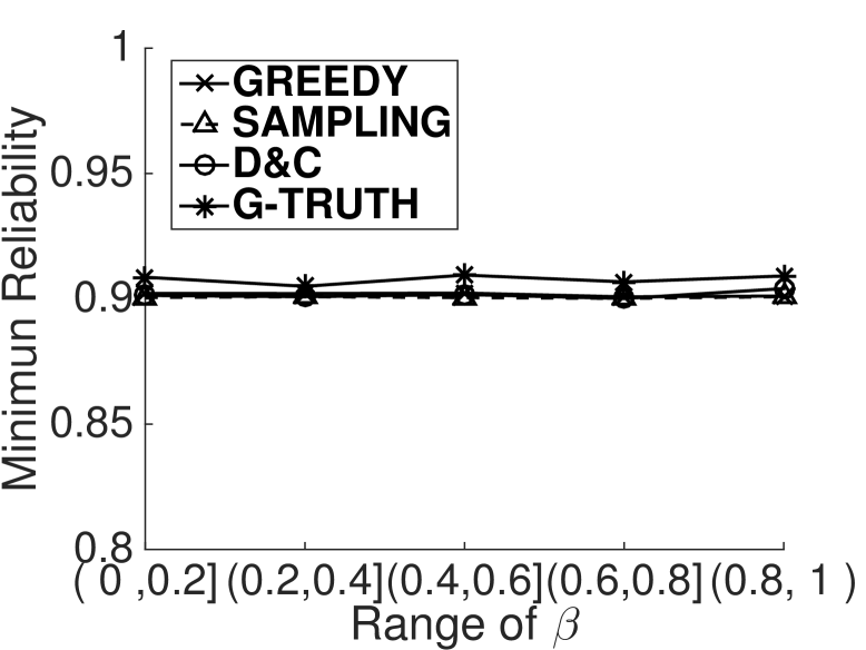
(a) Minimum Reliability

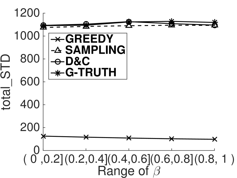
(b) Summation of Diversity

Figure 22: Effect of the Range of Requester-Specified Weight $\beta$

I. Cost Model of RDB-SC-Grid.

In this subsection, we illustrate how to set the best cell size $\eta$ based on our proposed cost model. In the sequel, we first propose a cost model to formalize the updating cost of the RDB-SC-Grid index. Then, we use the cost model to guide how to set $\eta$.

In general, the update cost of the RDB-SC-Grid index includes two parts, the cost of retrieving cells in the reachable area and that of checking every task in each candidate cell. Since workers do not move very far in general, we design the cost model based on the moving distance history. According to the moving history of workers, we can get the maximum moving distance, $L_{max}$, for all the workers. In the worst case, we need to check $\frac{\pi\cdot(L_{max}+\eta)^{2}}{\eta^{2}}$ cells. To estimate the number of tasks, $\overline{nt}$, in these cells, we use the power law [12] for the correlation fractal dimension $D_{2}$ of the tasks in the 2D data space. Then, we have $\overline{nt}=(N-1)\cdot(\pi\cdot(L_{max}+\eta)^{2})^{\frac{D_{2}}{2}}$. As the power law is applicable to both uniform data and nonuniform data in real world [12], we use it to estimate the tasks in the reachable area. With the cost of these two parts, we can get the updating cost, $cost_{update}$, of the RDB-SC-Grid index as follows:

$$cost_{update}=\frac{\pi\cdot(L_{max}+\eta)^{2}}{\eta^{2}}+(N-1)\cdot(\pi\cdot(L_{max}+\eta)^{2})^{\frac{D_{2}}{2}}.$$ (22)

Therefore, our goal is to set the best $\eta$ value for our grid index, such that $cost_{update}$ is minimized in Eq. (22). In particular, we take the derivative of $cost_{update}$ with respect to $\eta$, and let it equal to 0, that is, $\frac{\partial cost_{update}}{\partial\eta}=0$, which can be simplified as:

$$(L_{max}+\eta)^{D_{2}-2}\cdot\eta^{3}=\frac{2\pi^{1-D_{2}/2}\cdot L_{max}}{D_{2}\cdot(N-1)}.$$ (23)

Next, we can calculate $L_{max}$ and $D_{2}$ by collecting statistics from historical data, and then estimate a proper cell size $\eta$ according to Eq. (23). The resulting $\eta$ can minimize the updating cost of the RDB-SC-Grid index. When we do not have the historical data at the beginning, we can only assume that data are uniform such that $D_{2}=2$. As a result, we have $\eta=\sqrt[3]{\frac{L_{max}}{N-1}}$.

J. Figures on UNIFORM/SKEWED synthetic data.

We first present the effect of the range of Requester-Specified weight $\beta$ to our approaches on real data sets. Then, we show the effects of the parameters listed in Table 2 to our approaches on SKEWED synthetic data sets.

Effect of the Range of Requester-Specified Weight $\beta$. Figure 22 illustrates the effect of the range of requester-specified weight, $\beta$, on the reliability/diversity over real data set, where other parameters use their default values. In figures, when the range changes from $(0,0.2]$ to $(0.8,1)$, both reliability and diversity are not very sensitive, which indicates the robustness of the 3 approaches against weight $\beta$ for the spatial/temporal diversity. For all the tested ranges, both minimum reliability and diversity remain high (i.e., with reliability above 0.9, and the diversity of SAMPLING and D&C close to that of G-TRUTH).

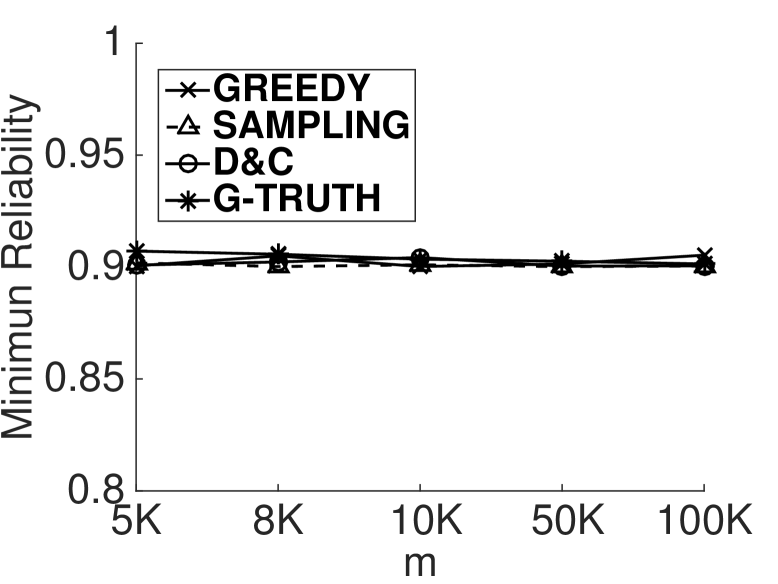
(a) Minimum Reliability

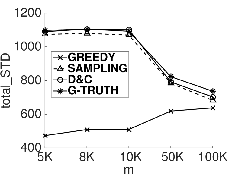
(b) Summation of Diversity

Figure 23: Effect of $m$ (SKEWED)

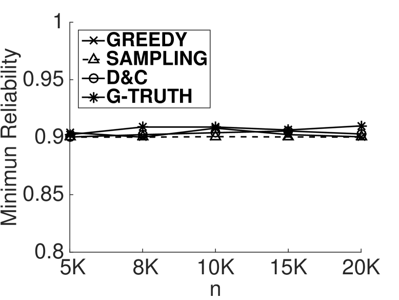
(a) Minimum Reliability

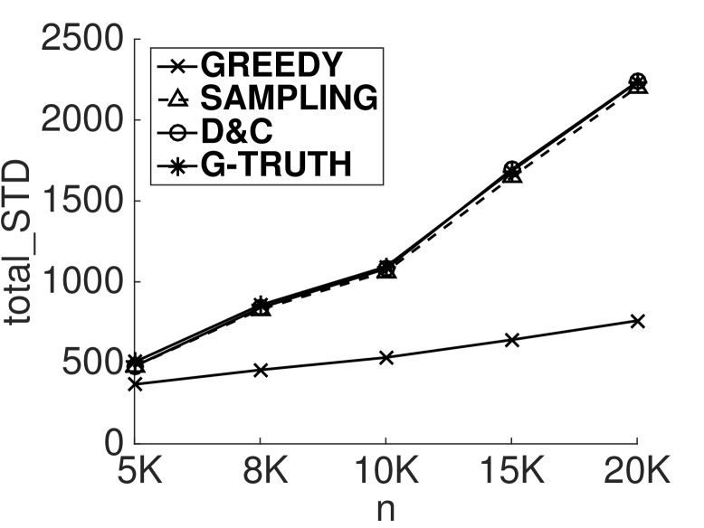
(b) Summation of Diversity

Figure 24: Effect of $n$ (SKEWED)

Effect of the number of the tasks, $m$ (SKEWED). Figure 23 shows the effect of the number of the tasks, $m$, using SKEWED synthetic data. In figures, the minimum reliability is not very sensitive to $m$. With the same reasons discussed in Section 8.3, when the number of tasks $m$ increases, the diversities of SAMPLING and D&C decrease, whereas that of GREEDY increases.

Effect of the number of the workers, $n$ (SKEWED). Figure 24 presents the effect of the number of the workers, $n$, on SKEWED synthetic data set. We can see that the minimum reliability is not sensitive to $n$. On the other hand, the diversities of all the approaches increase when $n$ becomes larger, which is same with the situation in UNIFORM data set. The reasons are same with the discussed reasons in Section 8.3.

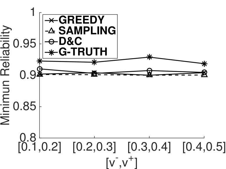
(a) Minimum Reliability

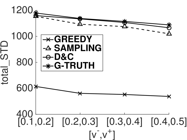
(b) Summation of Diversity

Figure 25: Effect of the Range of the Velocities $[v^{-},v^{+}]$ (UNIFORM)

Effect of the Range of Workers’ Velocities $[v^{-},v^{+}]$. (UNIFORM) Figure 25 reveals the effect of workers’ velocities range, $[v^{-},v^{+}]$, from $[0.1,0.2]$ to $[0.4,0.5]$. In figures, when the velocity in the range becomes higher, the minimum reliability remains high (i.e., around 0.9). Furthermore, the diversities of our approaches gradually decrease for higher velocity range. Intuitively, faster moving workers can potentially reach more tasks before their deadlines, which, however, lowers the total spatial/temporal diversity. Similarly, SAMPLING and D&C are much better than GREEDY in diversity perspective, and their diversities closely approach that of G-TRUTH.

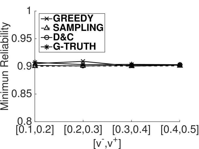
(a) Minimum Reliability

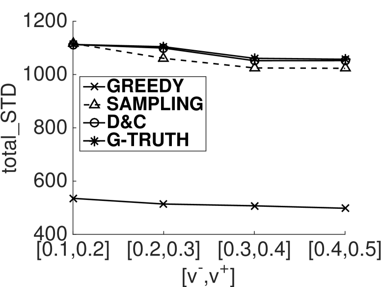
(b) Summation of Diversity

Figure 26: Effect of $[v^{-},v^{+}]$ (SKEWED)

Effect of Workers’ Velocity Range, $[v^{-},v^{+}]$ (SKEWED). Figure 26 shows the effect of workers’ velocity ranges over SKEWED synthetic data sets, where other parameters are set to default values. The minimum reliability of our approaches is not very sensitive to the velocity. For diversities, the results are similar to that on UNIFORM synthetic data. The same reason can explain why the diversities of SAMPLING, D&C, and G-TRUTH decrease, when workers’ moving speeds are improved.

Effect of the Range of Moving Angle, $(\alpha_{j}^{+}-\alpha_{j}^{-})$ (SKEWED). Figure 27 shows the experimental results by varying the range of workers’ moving angles, $(\alpha_{j}^{+}-\alpha_{j}^{-})$, from $(0,\pi/8]$ to $(0,\pi/4]$, on SKEWED synthetic data sets, where other parameters take default values. From figures, the minimum reliability is not very sensitive to the range of worker’ moving direction. As shown in Figure 27(b), SAMPLING and D&C can achieve much higher diversity, $total\_STD$, than GREEDY, and they have diversities similar to G-TRUTH.

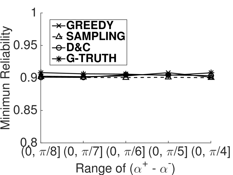
(a) Minimum Reliability

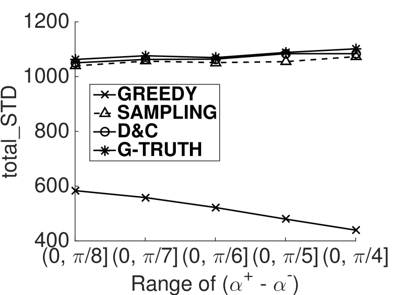
(b) Summation of Diversity

Figure 27: Effect of the Range of $(\alpha_{j}^{+}-\alpha_{j}^{-})$ (SKEWED)

References

- [1] https://www.google.com/maps/views/streetview.
- [2] http://mediaqv3.cloudapp.net/MediaQ_MVC_V3/.
- [3] https://foursquare.com.
- [4] https://www.waze.com.
- [5] https://www.mturk.com/mturk/welcome.
- [6] http://arxiv.org/abs/1412.0223.
- [7] http://www.gmissionhkust.com.
- [8] http://youtu.be/FfNoeqFc084.
- [9] Beijing city lab, 2008, data 13, points of interest of china in 2008. http://www.beijingcitylab.com.
- [10] F. Alt, A. S. Shirazi, A. Schmidt, U. Kramer, and Z. Nawaz. Location-based crowdsourcing: extending crowdsourcing to the real world. In NordiCHI 2010: Extending Boundaries, 2010.
- [11] S. Arora, S. Rao, and U. Vazirani. Expander flows, geometric embeddings and graph partitioning. JACM, 56(2):5, 2009.
- [12] A. Belussi and C. Faloutsos. Self-spacial join selectivity estimation using fractal concepts. TOIS, 16(2):161–201, 1998.
- [13] S. Börzsönyi, D. Kossmann, and K. Stocker. The skyline operator. pages 421–430, 2001.
- [14] M. F. Bulut, Y. S. Yilmaz, and M. Demirbas. Crowdsourcing location-based queries. In 2011 IEEE International Conference on PERCOM Workshops, pages 513–518, 2011.
- [15] Z. Chen, R. Fu, Z. Zhao, Z. Liu, L. Xia, L. Chen, P. Cheng, C. C. Cao, and Y. Tong. gmission: A general spatial crowdsourcing platform. Proceedings of the VLDB Endowment, 7(13), 2014.
- [16] C. Cornelius, A. Kapadia, D. Kotz, D. Peebles, M. Shin, and N. Triandopoulos. Anonysense: privacy-aware people-centric sensing. In Proceedings of the 6th international conference on Mobile systems, applications, and services, 2008.
- [17] N. N. Dalvi and D. Suciu. Efficient query evaluation on probabilistic databases. VLDBJ, 16(4), 2007.
- [18] D. Deng, C. Shahabi, and U. Demiryurek. Maximizing the number of worker’s self-selected tasks in spatial crowdsourcing. In Proceedings of the 21st SIGSPATIAL GIS, pages 314–323, 2013.
- [19] L. Kazemi and C. Shahabi. A privacy-aware framework for participatory sensing. SIGKDD Explorations Newsletter, 13(1):43–51, 2011.
- [20] L. Kazemi and C. Shahabi. Geocrowd: enabling query answering with spatial crowdsourcing. In Proceedings of the 21st SIGSPATIAL GIS, pages 189–198, 2012.
- [21] S. Mertens. The easiest hard problem: Number partitioning. Computational Complexity and Statistical Physics, page 125, 2006.
- [22] M. L. Yiu and N. Mamoulis. Efficient processing of top- dominating queries on multi-dimensional data. In VLDB, pages 483–494, 2007.
- [23] J. Yuan, Y. Zheng, X. Xie, and G. Sun. Driving with knowledge from the physical world. In Proceedings of the 17th SIGKDD, 2011.
- [24] J. Yuan, Y. Zheng, C. Zhang, W. Xie, X. Xie, G. Sun, and Y. Huang. T-drive: driving directions based on taxi trajectories. In Proceedings of the 18th SIGSPATIAL GIS, pages 99–108, 2010.