Spin dynamics of the anisotropic spin-1 antiferromagnetic chain at finite magnetic fields

Abstract

We present results of a study of the antiferromagnetic spin-1 chain, subject to the simultaneous presence of single-ion anisotropy and external magnetic fields. Using quantum Monte-Carlo based on the stochastic series expansion method we first uncover a rich quantum phase diagram comprising Néel, Haldane, Luttinger liquid, and large anisotropy phases. Second, we scan across this phase diagram over a wide range of parameters, evaluating the transverse dynamic structure factor, which we show to exhibit sharp massive modes, as well as multi particle continua. For vanishing anisotropy and fields, comparison with existing results from other analytic and numerical approaches shows convincing consistency.

I Introduction

Ever since Haldane’s conjecture Haldane1983 on the difference between even and odd half-integer Heisenberg antiferromagnetic spin chains (HAFC), the spin-1 HAFC (S1-HAFC)

$$H=J\sum_{n}\vec{S}_{n}\cdot\vec{S}_{n+1}-h\sum_{n}S_{n}^{z}+D\sum_{n}(S_{n}^{z})^{2},$$ (1)

has been considered to be one of the fundamental models of low-dimensional quantum magnetism. Here, the first term on the right hand side of (1) refers to the bare chain, with antiferromagnetic exchange interaction $J$ and spin-1 operators $\vec{S}_{n}$ at sites $n$, and the remaining terms capture common perturbations by single-ion anisotropy $D$ and external longitudinal magnetic fields $h$.

For the isotropic case at zero magnetic field, i.e. $D=0$ and $h=0$, both, static and dynamic properties of the S1-HAFC have been investigated extensively using various theoretical and numerical methods Kolezhuk2004 . On the zone boundary at $q=\pi$, its lowest-lying excitation is a massive ’single-magnon’ mode which displays the famous Haldane gap of $\Delta\simeq 0.41J$ Nightingale1986 ; White1993 Near $q=0$ the spectrum comprises primarily a two-particle continuum of small spectral weight Gomez-Santos1989 ; Affleck1992 ; Yamamoto1993 ; White1993 This continuum is separated from the ground state by $2\Delta$. Finally, the next to dominant excitations near $q=\pi$ are contained in a three-particle continuum starting at $3\Delta$. Theoretically these excitations have been obtained from several analytic approaches, eg., mean-field theory Affleck1992 , the nonlinear $\sigma$ model (NL$\sigma$M) Affleck1999 , as well as numerical methods, eg., quantum Monte-Carlo (QMC) Takahashi1989 ; Deisz1990 ; Meshkov1993 ; Yamamoto1997 , density matrix renormalization group (DMRG) White1993 ; White2008 .

Experimentally, the massive magnon at $q=\pi$ has been confirmed irrevocably, however the two-, and in particular the three-particle continua remain a matter of active research Ma1992 ; Zaliznyak2001 ; Kenzelmann2001 .

Most spin-1 chain compounds, such as NENP Renard1987 ; Regnault1994 , DTN Paduan-Filho2004 ; Zapf2006 , NENC Orendac1995 , NDMAP Honda1998 ; Zheludev2001 , and NDMAZ Honda1997 ; Zheludev2001a display sizable anisotropy $D$ and even the well studied prototype material $CsNiCl_{3}$ Steiner1987 ; Kenzelmann2002 has $D\neq 0$. Therefore, it is of great interest to analyze the ground state properties and the evolution of the excitation spectrum as a function of anisotropy. In addition, many experimental studies, including neutron scattering Facility1994 ; Zheludev2004 (NS), electron-spin resonance Sieling2000 ; Zvyagin2008 (ESR), nuclear magnetic resonance Chiba1991 ; Takigawa1996 ; Haga2000 (NMR), and thermal transport Sologubenko2008 are performed at finite magnetic fields.

For vanishing magnetic field several studies have already been performed regarding the quantum phases as a function of the anisotropy Nijs1989 ; Schulz1986 ; Kennedy1992 ; Chen2003 ; DegliEspostiBoschi2003 ; Tzeng2008a ; Hu2011 ; Furuya2011 ; Albuquerque2009 . Similarly the magnetic field driven transition into a Luttinger liquid (LLQ) phase Affleck1991 ; Golinelli1992 ; Konik2002 at $D=0$ is well investigated. At finite $D$ and $h$ there are some studies with planar or a combination of planar and axial magnetic fields and additional other components of anisotropies Pollmann2010 ; Gu2009 ; Sengupta2007 , still, too little is known about the region of finite $D$ and $h$ for the Hamiltonian (1). Therefore, the central goal of this paper is to shed more light onto the combined impact and interplay between finite anisotropy and magnetic fields in S1-HAFCs, both regarding static and dynamic properties.

The paper is organized as follows. In section II we uncover and discuss the quantum phase diagram of (1) over a substantial range of $D$ and $h$. In section III we detail our results for the transverse dynamic structure factor (tDSF) and analyze its evolution in terms of anisotropy and magnetic fields. Where available comparison to other methods, in particular NL$\sigma$M model calculations Affleck1992 ; Affleck1999 and tDMRG White2008 will be provided. We conclude and summarize our findings in Sec.IV. Appendix A contains a short summary of the quantum Monte-Carlo method we use.

II Quantum Phase diagram

In this section, and before analyzing its dynamical properties, we will evaluate the ground state phase diagram of the chain versus single-ion anisotropy and magnetic field.

At zero magnetic field, the phase diagram in terms of anisotropy has been already investigatedSchulz1986 ; Nijs1989 ; Kennedy1992 ; Chen2003 . It consists of a Néel, a Haldane, and a large-D phase. The transition from the Néel to the Haldane phase is of Ising type, while that from the Haldane to large-D phase is of Gaussian type. The critical values $D_{c}$ for the transition between these phases have been determined using various numerical methods including exact diagonalization Chen2003 , DMRG DegliEspostiBoschi2003 ; Tzeng2008a ; Hu2011 , series expansions and QMC Albuquerque2009 . Although there are slight quantitative differences between the results from different methods for $D_{c}$, it is generally believed that the transition between the Néel and Haldane phase occurs around $D_{NH}\simeq-0.31J$ and that between the Haldane and large-D phase around $D_{HL}\simeq 1.0J$ DegliEspostiBoschi2003 ; Tzeng2008a ; Albuquerque2009 ; Hu2011 .

All three phases, Néel, Haldane, and large-D, are gapful. It is known that the spin gap of Haldane phase decreases upon increasing the easy-plane anisotropy up to the critical point $D_{c}$ and increases again afterwards, however, one remains in a gapful state Hu2011 . Applying an external magnetic field can also suppress the spin gap of the chain. Affleck1991 ; Golinelli1992 ; Konik2002 . This means that at large enough fields, the S1-HAFC enters a LLQ phase. Now the question is how and where exactly the gap closes. In other words the boundaries of this LLQ phase are to be obtained. Here we will quantify this and establish how in general the quantum phase diagram evolves within the $D,h$ plane.

There are several ways to determine the extent of the Haldane phase. One is to evaluate the string order parameter Nijs1989 ; Kennedy1992 , which is a nonlocal probe of the topological order. This order parameter is fragile with respect to perturbations which break rotation symmetry, while keeping other symmetries such as time-reversal, parity and translation symmetries intact Anfuso2007 ; Gu2009 ; Pollmann2010 . Since both, the Haldane and large-D phases are gaped while the LLQ formed between them is gapless, another and rather direct way to determine the boundary between these phases is to scan the energy gap versus $D$, fixing eg. $h$. To obtain the gap, we first evaluate the uniform spin susceptibility in terms of temperature $\chi(T)$. We then extract the gap by fitting the low-temperature values of $\chi(T)$ to $\chi(T)\approx e^{-\Delta/T}P_{k}^{l}(T)/T$, where $P_{k}^{l}(T)$ is a Padé approximant of order $[k,l]$. In principle, finite size scaling of the gap determined this way should be performed, in particular because of critical behavior near the transition points Barber1983 . In pratice however and because of the additional approximation introduced by the Padé fitting we simple use a sufficiently large system of $512$ sites. The lowest temperature we have considered is $T=0.0078J$.

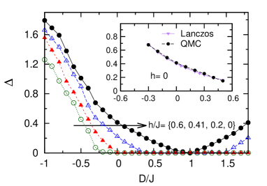
Figure 1: Spin gap of the spin-1 chain in terms of single-ion anisotropy for different external magnetic fields. Inset: for zero magnetic field, the spin gap in terms of single-ion anisotropy obtained from QMC and Lanczos method is shown. Lanczos data are extracted from Ref.Furuya2011, . The system size and the lowest temperature considered for QMC data are $L=512$ and $T=0.0078$.

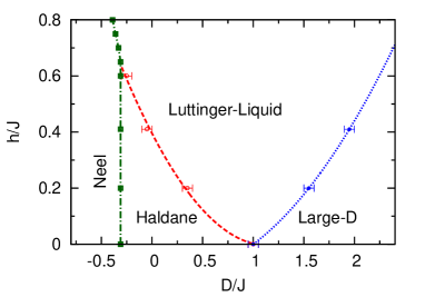
Figure 2: Quantum phase diagram of the spin-1 Heisenberg chain versus single-ion anisotropy and magnetic field. The error bars of the transition points are equal to the distance between two sequential values of $D/J$ in each of the two procedures, gap or Néel order study. In case of Haldane-Néel case, these error bars are smaller than the symbols.

Fig. 1 summarizes all gaps $\Delta(D,h)$ extracted from the preceding procedure, both, versus $D$ and for several magnetic fields. For each gap, the Padé fitting errors are found to be within the QMC’s error bars which are of the order of $10^{-4}$. Above the critical field $h_{c}(D)$, there are two points of gap closure and reopening, which we identify with the transition from the Haldane into the LLQ, and from the LLQ into the large-D phase. At $D=D_{HL}$ the latter two points have to merge at $h=0$ where the direct transition from the Haldane to large-D occurs without accessing a LLQ phase. The gaps in Fig. 1 display some clearly visible, albeit small, noise. This is not related to QMC, or Padé approximant errors. In fact, for each individual gap extracted, the Padé fitting errors are within the QMC’s error bars which are of the order of $10^{-4}$. Rather, the noise is a consequence of the arbitrariness in choosing the upper cut-off for the temperature range, used in Padé fitting $\chi(T)$. This noise translates into an error for the phase boundaries, which we find to dominate any corrections from finite scaling. This justifies our neglect of the latter a posteriori.

Previous studies Furuya2011 have analyzed the spin gap for $h=0$ using Lanczos spectra of small systems $L{\leq}20$, over a restricted range of $D_{NH}{<}D{<}D_{HL}$. As compared to QMC, finite size effects are a relevant issue for this approach, and careful scaling analysis is necessary, in particular for $D$ in the vicinity of $D_{HL}$, where gap closure occurs. The inset of Fig. 1, compares our thermodynamic QMC gap with that obtained from extrapolating to $L\rightarrow\infty$ in Ref. Furuya2011, . The agreement is satisfying.

In Fig. 2 we collect the gap closure points obtained from Fig. 1 as part of a quantum phase diagram versus $D$ and $h$. The transition points are regarded as the midpoints of the two sequential $D$ values for one of which $\Delta$ is finite (gapped phase) while for the other one $\Delta\approx 0$ (gapless phase). Since the distance between two sequential $D/J$ values is $0.1$, the uncertainty for the transition points is $\pm 0.05$. The lines connecting the points are low order polynomials fitted to the points. This figure also shows a transition from the Neél to the Haldane phase, to which we turn now. Since both of the latter phases are gapful, the transition line cannot be obtained from a study of gap closures. Instead, we use that the long-range staggered spin-correlation is an order parameter of the Neél phase, and remains finite therein, while it decays in the Haldane phase Charrier2010 . This has been applied previously to characterize the Haldane phase as a function exchange anisotropy in the $XXZ$ spin-1 chain Su2012 . The staggered spin-correlation reads

$${\cal O}^{\,z}_{\textrm{N}}(i,j)=(-1)^{i-j}\langle S^{z}_{i}S^{z}_{j}\rangle,$$ (2)

and Neél ordering implies $O^{\,z}_{\textrm{N}}=\lim_{|i-j|\rightarrow\infty}{\cal O}^{\,z}_{\textrm{N}}(i,j)\neq 0$.

Fig. 3 displays our results for ${\cal O}^{\,z}_{\textrm{ N}}(0,L)$ for $L=512$. In view of the rather large system, we refrain from finite size scaling analysis, and approximate ${\cal O}^{\,z}_{\textrm{ N}}(0,512)\simeq O^{\,z}_{\textrm{N}}$. We identify the phase transition point with the average value between the smallest $D$ at which $O^{\,z}_{\textrm{N}}\approx 0$, where we are in the Haldane phase, and the largest $D$ point at which $O^{\,z}_{\textrm{N}}$ is finite, where we are in the Neél phase. The error in this case is $\pm 0.005$. From this, and for $h=0$ we obtain a transition point at $D_{NH}\approx-0.305J$, which is satisfyingly close to the values obtained by DMRG in Refs. Tzeng2008a, ; Hu2011,

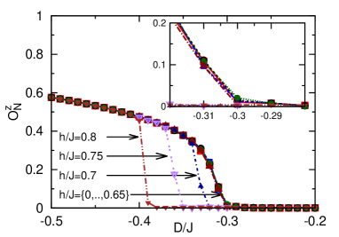
Figure 3: Néel order parameter is shown as a function of anisotropy for different magnetic fields. The inset shows the transition point between Haldane and Neél phase for $h/J={0,..,0.65}$ . The system size and the temperature considered here are $L=512$ and $T=0.01J$.

The main message of Fig. 3 is contained in the remarkable evolution of $O^{\,z}_{\textrm{N}}$ and the quantum critical point with magnetic field. As the figure shows, the critical value of $D_{NH}(h)$ is independent of the field up to a critical value $\tilde{h/J}\approx 0.65$, below which all curves for $O^{\,z}_{\textrm{N}}$ collapse onto a single one. Adding $D_{NH}(h)$ into Fig. 2 shows that the point ($D_{NH}$,$\tilde{h}$) lies on the extrapolated line, approximating the boundary of the LLQ phase. From the slope of this phase boundary, and since $O^{\,z}_{\textrm{N}}$ has to be zero in the LLQ phase, further increasing the field, the value of $D_{NH}(h)$ must decrease for $h{>}\tilde{h}$. This is consistent with $O^{\,z}_{\textrm{N}}$ in Fig. 3. In fact, as is obvious from the green squares in Fig. 2, to within the uncertainty of the LLQ phase boundary, the Neél-Haldane transition is replaced by a direct transition from the Neél to the Luttinger phase for $h>\tilde{h}$.

III Dynamic structure factor

In this section we discuss the transverse dynamic structure factor $\bf{S(q,\omega)}$. We will be interested in the Neél, Haldane, and Luttinger phase. For this we analyze several values of magnetic field and anisotropy, as shown in Fig. 2.

First, we focus on the field dependence of $\bf{S(q,\omega)}$ at the isotropic point. Results for this are shown in the contour plots of Fig. 4. At zero magnetic field most of the spectral weight is contained in a single, well defined excitation, which is clearly visible in Fig. 4a). Most of the spectral weight of this so-called one magnon mode resides at large momenta near $q=\pi$ and decreases rapidly towards lower momenta, where we find that the integrated weight is proportional to $q^{2}$ as $q\rightarrow 0$. At finite magnetic field, the two triplet branches which can be reached $\Delta S=+1$ transitions, split according to their Zeeman energy. For small fields, this splitting is manifest through a broadening of the one-magnon line, while the intensity decreases, as can been seen from Fig. 4b) and by comparing their intensity scales. If the Zeeman splitting is larger than the broadening of the one-magnon excitations due to thermal, interaction, and MaxEnt effects, then the splitting is directly visible, as in Fig. 4c). In that panel, the Zeeman energy has been chosen identical to the Haldane gap. As can be seen, at this point the maximum intensity of the lower branch extrapolates to zero energy at $q=\pi$, i.e. the gap closes, consistent with entering the LLQ phase.

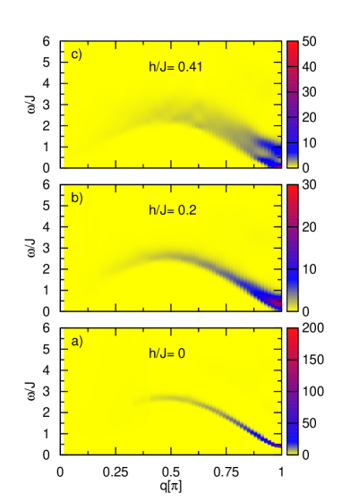
Figure 4: Contour plot of the transverse dynamic structure factor of the isotropic spin-1 chain as a function of frequency $\omega$ and wave vector $q$ for three different magnetic fields $h=0,0.2,$ and $0.41J$. The system size of the chain for all cases is $L=128$ and temperature is set to $T=0.1J$.

Next we focus on a more detailed discussion of 2D cuts of the spectra versus $D$ and $h$ at small and large momenta. The main motivation for this is, that apart from the one-magnon excitation, there are also multi-particle continua present in the spectrum. While the former are most dominant at large momenta, the latter exhibit very small spectral weight, which remains invisible in contour plots of the full BZ, and can be observed best at small momenta. Therefore we have plotted cuts through the tDSFs at various anisotropies and magnetic fields in Fig. 5, which allows to clearly see the shape and weight of the spectra, despite very large differences in their absolute scales in different frequency and momentum regions. We have chosen three magnetic fields $h=0$, $0.2$, $0.41J$ and five different anisotropies, $D=-0.2,-0.5,0,0.2,0.5$ ranging from easy-axis to easy-plane anisotropies. For each of these cases two wave vectors have been considered, i.e., $q=\pi$ (right panel), and $q=\pi/64$ (left panel), which is the smallest on the system for which we have evaluated the tDSF, i.e. $L=128$.

We start with the isotropic case at small momenta, Fig. 5c). At zero magnetic field it is dominated by a peak at zero frequency. This central peak intensity stems from $\Delta S=+1$ transitions within thermally excited states and decreases as the tempearture is lowered. In addition, there exists a continuum of very small weight at higher frequencies, which however is not observable on the scale of this plot. We emphasize, that this observation is rather distinct from expectations White2008 at zero temperature, where the latter multi-magnon spectrum should dominate the spectrum at low-momentum displaying a gap of twice the Haldane gap. Increasing the wave vector, the weight of the continuum gets larger as we will discuss later. Increasing the magnetic field, the central peak and the continuum shift to larger frequencies, with an energy scale set by the Zeeman energy.

Turning to finite anisotropy either of easy-axis type in Fig. 5a) and b), or of easy-plane type in Fig. 5d) and e), a shifting the dominant weight of spectrum to larger frequencies is clearly visible. In addition to that an interesting interplay between the effects of anisotropy and magnetic field on the spectrum can be observed, which differs between the two kinds of anisotropies. While in the case of easy-plane anisotropy, the magnetic field only slightly shifts the weight of the spectrum, in the case of easy-axis anisotropy, a splitting of the dominant peak result which increases with increasing field.

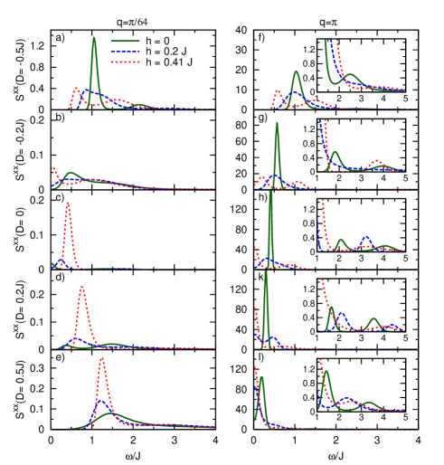
Figure 5: Transverse dynamic structure factor of the spin-1 chain as a function of frequency at two q vectors for different anisotropies and magnetic fields is plotted. The system size of the chain for all cases is $L=128$ and temperature is set to $T=0.1J$.

Another interesting feature is the evolution of the spectrum versus anisotropy upon switching from the Haldane into the Neél phase. In the former we expect a rather broad continuum from multiparticle excitations at small momentum, while in the latter a single dominant excitation should occur, representing one-magnon excitations, which may however still exhibit some broadening due to finite temperature and interaction effects. Exactly this can be seen in going from Fig. 5b) to a), where also the overall amplitude scale increases by one order of magnitude in going from b) to a). At $q=\pi$, however, the spectrum gets broadened, as one goes from the Haldane into the Neél phase by changing the anisotropy.

Moving to spectra at $q=\pi$, one can clearly see the sharp magnon peak which dominates the spectrum at all anisotropies and magnetic fields. At zero magnetic field, the peak position which is a fingerprint of spin gap shifts towards lower frequencies as we go from strong easy-axis anisotropy $D=-0.5J$ in Fig. 5f) to strong easy-plane one $D=0.5J$ in Fig. 5l). We find that in all cases studied there is good agreement between the position of the peaks maximum and the thermodynamic spin gaps which we have obtained in section II. As can be seen from 5f) through l) the monotonous behavior of the spectrum in terms of anisotropy remains intact, even at finite magnetic field, but it is accompanied by a splitting of the dominant peak due to Zeeman effect as we have already mentioned in the context of Fig. 4. The splitting increases until the lower branch reaches its maximum at zero frequency, at $h=h_{c}(D)$, where the LLQ is entered. Increasing the magnetic field beyond $h_{c}(D)$ leads to an accumulation of spectral weight at zero frequency and a depletion and smearing of the upper Zeeman peak. This behavior is clearly visible in 5 k) and l). In view of the phase diagram Fig. 2, and because the largest field we consider in Fig. 5 is $h_{c}(0)$, the maximum of the lower brance has to stay above $\omega=0$ for $D<0$, which is exactly what we find in Fig. 5g) and f).

In addition to the dominant single-magnon peak at $q=\pi$, we find a very weak multi-particle continuum at higher frequencies. This is most likely due to three-magnon excitations, as proposed in Refs. Affleck1999, ; White2008, . In view of the relative intensities, it is remarkable, that our MaxEnt calculations are able to resolve this continuum with respect to the single-magnon peak. Moreover these results hint as to why experimental inelastic struture factor determination of such continua have failed so far Zaliznyak2001 .

Finally we contrast our findings with those from other approaches, namely the NL$\sigma$ model and a free boson method Affleck1992 ; Affleck1999 , as well as tDMRG White2008 . In Fig. 6 results are shown for two momenta, i.e. $q=\pi/10$ and $q=\pi$. For the former, the spectrum is dominated by only the two-particle continuum and Fig. 6a) demonstrates good qualitative agreement between all different methods. Regarding the quantitative difference of the QMC to the other approaches, it is clear that the sharp onset of the continuum is smeared. The reason for this is twofold, primarily it results from the fact that our QMC is a finite temperature result, at $T=0.1J$, while all other methods refer to zero temperature. Additionally MaxEnt cannot be avoided to introduce additional smoothing of any QMC spectrum. The spectrum at $q=\pi$ is shown in Fig. 6b). As discussed previously, this spectrum contains two largely separted intensity scales, one due to the single-magnon mode, the other due to the three-particle continuum. For the former and as for Fig. 6a) we see convincing agreement between all approaches for the locations of the magnon peak, including some finite temperature and MaxEnt broadening of the QMC. Turning to the high energy contiunuum at this wave vector, we first note that all methods result in a comparable spectral intensity, however clear qualitative differences are obvious. While both, NL$\sigma$ model and tDMRG display only a single ’hump’, QMC results in two, moreover, while the tDMRG and QMC spectrum remains confined to $1.5\lesssim\omega/J\lesssim 5.5$, the spectrum from the NL$\sigma$ model continues up to much higher energies. The origin of these differences remains unclear at present.

IV Conclusions

We have used QMC to study the antiferromagnetic spin-1 chain subject to the simultaneous presence of single-ion anisotropy and external magentic fields. The focus has been on two issues, namely the quantum phase diagram and the transverse dynamic structure factor. We have uncovered a rich set of quantum phases within the parameter range investigated, comprising Neél, Haldane, Luttinger-liquid, and large anisotropy regimes. All transitions where found to be of second order, as determined from either closures of spin gaps, or by direct evaluation of order parameters.

Based on the phase diagram, we have determined the transverse spin dynamics, covering the complete Brillouin zone, and varying the system parameters to access the excitations within the Neél, Haldane, Luttinger-liquid states. First, we have studied the spectral weight, splitting and dispersion of the single-magnon mode, known from the standard antiferromagnetic spin-1 chain, however versus anisotropy and external fields. Second we have provided clear evidence for multi particle continua with partially very small spectral weight and investigated their evolution with momentum and system parameters.

Finally we have shown that our finite temperature spectra are consistent with existing zero temperature results from other analytic as well as numerical approaches. We hope that our findings may inspire additional experimental studies using inelastic neutron scattering on spin-1 chain materials.

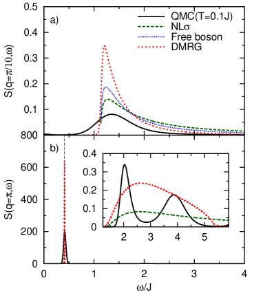
Figure 6: Dynamic structure factor of the isotropic chain at zero magnetic field for two wave vectors ($q=\pi/10,\pi$) and different methods is shown. For QMC data, the temperature is set to $T=0.1J$ while for other data which are extracted from Refs. Affleck1992, ; Affleck1999, ; White2008, the temperature is set to zero.

Appendix A Method

All physical quantities in this paper are obtained using the stochastic series expansion (SSE) method, pioneered by Sandvik $et\>al.$ Sandvik1992 ; Sandvik1999 ; Syljuasen2002 . This method is based on importance sampling of the high temperature series expansion of the partition function

$$Z=\sum_{\alpha}\sum_{n}\sum_{S_{n}}\frac{(-\beta)^{n}}{n!}\left\langle\alpha\right|\prod_{k=1}^{n}H_{a_{k},b_{k}}\left|\alpha\right\rangle\,$$ (3)

where $\beta$ is inverse temperature $1/T$ and $H_{1,b}=1/2-S_{b1}^{z}S_{b2}^{z}$ and $H_{2,b}=(S_{b1}^{+}S_{b2}^{-}+S_{b1}^{-}S_{b2}^{+})/2$ are spin diagonal and off-diagonal bond operators. $|\alpha\rangle=\left|S_{1}^{z},\ldots,S_{N}^{z}\right\rangle$ refers to the $S^{z}$ basis and $S_{n}=[a_{1},b_{1}][a_{2},b_{2}]\ldots[a_{n},b_{n}]$ is an index for the operator string $\prod_{k=1}^{n}H_{a_{k},b_{k}}$. This string is Metropolis sampled, using two types of update, diagonal updates which change the number of diagonal operators $H_{1,b_{k}}$ in the operator string and directed loop updates which change the type of operators $H_{1,b_{k}}\leftrightarrow H_{2,b_{k}}$. For nonfrustrated spin-systems the latter update comprises an even number of off-diagonal operators $H_{2,b_{k}}$, ensuring positivity of the transition probabilities.

The dynamic structure factor, is obtained from QMC in real space $i,j$ and at imaginary time $\tau$. Following Ref. Sandvik1992, we consider

$$S_{i,j}\left(\tau\right)=\Bigg{\langle}\sum_{p,m=0}^{n}\frac{\tau^{m}(\beta-\tau)^{n-m}n!}{\beta^{n}(n+1)(n-m)!m!}\times\phantom{aaa}$$

$$S_{i}^{+}(p)S_{j}^{-}(p+m)\Bigg{\rangle}_{W}~{},$$ (4)

where $\langle\ldots\rangle_{W}$ refers to the Metropolis weight of an operator string of length $n$ generated by the stochastic series expansion of the partition function Sandvik1999 ; Syljuasen2002 , and $p,m$ are positions in this string and $S_{i}(p)$ refers to the intermediate state $\left|\alpha(p)\right\rangle=\prod^{p}_{k=1}H_{a_{k},b_{k}}\left|\alpha\right\rangle$.

From (4) we proceed by performing a Fourier transformation into momentum space

$$S({\bf q},\tau)=\sum_{a}e^{i{\bf q}\cdot{\bf r}_{a}}S_{a,0}(\tau)/L$$ (5)

with $L$ being the system-size. The sought for form of the dynamical structure factor in frequency and momentum space finally results from analytic continuation to real frequencies based on the inversion of

$$S({\bf q},\tau)=\frac{1}{\pi}\int_{0}^{\infty}d\omega S_{\perp}({\bf q},\omega)K(\omega,\tau),$$ (6)

with a kernel $K(\omega,\tau)=e^{-\tau\omega}+e^{-(\beta-\tau)\omega}$.

The preceding inversion is an ill-posed problem, for which maximum entropy methods (MaxEnt) have proven to be well suited. We have applied Bryan’s algorithm for our MaxEnt J.Skilling1984 ; Jarrell1996 . In a nutshell this method minimizes the functional $Q=\chi^{2}/2-\alpha\sigma$, with $\chi$ being the covariance of the QMC data with respect to the MaxEnt trial spectrum $S({\bf q},\omega)$. Overfitting is prevented by an entropy term $\sigma=\sum_{\omega}S({\bf q},\omega)\ln[S({\bf q},\omega)/m(\omega)]$. We have used a flat default model $m(\omega)$ which is iteratively adjusted to match the zeroth moment of the trial spectrum. The optimal spectrum follows from the weighted average of $S({\bf q},\omega)$ with the probability distribution $P[\alpha|S({\bf q},\tau)]$ adopted from Ref. J.Skilling1984 . Using static structure factors evaluated by independent QMC runs, we have checked that all spectra obtained from our MaxEnt, perfectly fulfill sum rules.

References

- (1) F. D. M. Haldane, Phys. Rev. Lett. 50, 1153 (1983).
- (2) H.-J. Mikeska and A. K. Kolezhuk, in Quantum magnetism, edited by U. Schollwöck, J. Richter, D. J. J. Farnell, and R. F. Bishop (Springer, 2004), Vol. 645, pp. 1–83.
- (3) M. P Nightingale and H. W. J. Blöte, Physical Review B 33, 659 (1986).
- (4) S. R White and D. A. Huse, Physical Review B 48, 3844 (1993).
- (5) G. Gómez-Santos, Physical Review Letters 63, 790 (1989).
- (6) I. Affleck and R. A. Weston, Physical Review B 45, 4667 (1992).
- (7) S. Yamamoto and S. Miyashita, Physical Review B 48, 9528 (1993).
- (8) M. D. P. Horton and I. Affleck, Phys. Rev. B 60, 11891 (1999).
- (9) M. Takahashi, Physical Review Letters 62, 2313 (1989).
- (10) J. Deisz, M. Jarrell, and D. L. Cox, Physical Review B 42, 4869 (1990).
- (11) S. V. Meshkov, Physical Review B 48, 6167 (1993).
- (12) S. Yamamoto and S. Miyashita, Physics Letters A (1997).
- (13) S. R White and I. Affleck, Phys. Rev. B 77, 134437 (2008).
- (14) Shaolong Ma, Collin Broholm, Daniel H. Reich, B. J. Sternlieb, and R. W. Erwin, Physical Review Letters 69, 3571 (1992).
- (15) I. A. Zaliznyak, S.-H. Lee, and S. V. Petrov, Physical Review Letters 87, 017202 (2001).
- (16) M. Kenzelmann et al., Phys. Rev. Lett. 87, 017201 (2001).
- (17) J. P. Renard et al., Europhysics Letters (EPL) 3, 945 (1987).
- (18) L. P. Regnault, I. Zaliznyak, J. P. Renard, and C. Vettier, Physical Review B 50, 9174 (1994).
- (19) A. Paduan-Filho, X. Gratens, and N. F. Oliveira, Physical Review B 69, 020405 (2004).
- (20) V. Zapf et al., Physical Review Letters 96, 077204 (2006).
- (21) M. Orendáč et al., Physical Review B 52, 3435 (1995).
- (22) Z. Honda, H. Asakawa, and K. Katsumata, Physical Review Letters 81, 2566 (1998).
- (23) A. Zheludev, Y. Chen, C. L. Broholm, Z. Honda, and K. Katsumata, Physical Review B 63, 104410 (2001).
- (24) Z. Honda et al., Journal of Physics: Condensed Matter 9, L83 (1997).
- (25) A. Zheludev et al., Europhysics Letters (EPL) 55, 868 (2001).
- (26) M. Steiner et al., Journal of Applied Physics 61, 3953 (1987).
- (27) M. Kenzelmann et al., Phys. Rev. B 66, 024407 (2002).
- (28) R. Facility, 50, (1994).
- (29) A. Zheludev, S. M. Shapiro, Z. Honda, K. Katsumata, B. Grenier, E. Ressouche, L.-P. Regnault, Y. Chen, P. Vorderwisch, H.-J. Mikeska, and A. K. Kolezhuk, Physical Review B 69, 054414 (2004).
- (30) M. Sieling et al., Physical Review B 61, 88 (2000).
- (31) S. Zvyagin et al., Physical Review B 77, 092413 (2008).
- (32) M. Chiba, Y. Ajiro, H. Kikuchi, T. Kubo, and T. Morimoto, Physical Review B 44, 2838 (1991).
- (33) M. Takigawa, T. Asano, Y. Ajiro, M. Mekata, and Y. J. Uemura, Physical Review Letters 76, 2173 (1996).
- (34) N. Haga and S.-i. Suga, Journal of the Physics Society Japan 69, 2431 (2000).
- (35) A. Sologubenko et al., Physical Review Letters 100, 137202 (2008).
- (36) M. den Nijs and K. Rommelse, Physical Review B 40, 4709 (1989).
- (37) H. J. Schulz, Physical Review B 34, 6372 (1986).
- (38) T. Kennedy and H. Tasaki, Communications in mathematical physics 484, 431 (1992).
- (39) W. Chen, K. Hida, and B. C. Sanctuary, Physical Review B 67, 104401 (2003).
- (40) C. Degli Esposti Boschi, E. Ercolessi, F. Ortolani, and M. Roncaglia, The European Physical Journal B - Condensed Matter 35, 465 (2003).
- (41) Y.-C. Tzeng and M.-F. Yang, Physical Review A 77, 012311 (2008).
- (42) S. Hu, B. Normand, X. Wang, and L. Yu, Physical Review B 84, 220402 (2011).
- (43) S. C. Furuya, T. Suzuki, S. Takayoshi, Y. Maeda, and M. Oshikawa, Physical Review B 84, 180410 (2011).
- (44) A. F. Albuquerque, C. J. Hamer, and J. Oitmaa, Physical Review B 79, 054412 (2009).
- (45) I. Affleck, Physical Review B 43, 3215 (1991).
- (46) O. Golinelli, T. Jolicoeur, and R. Lacaze, Physical Review B 45, 9798 (1992).
- (47) R. M. Konik and P. Fendley, Physical Review B 66, 144416 (2002).
- (48) F. Pollmann, A. M. Turner, E. Berg, and M. Oshikawa, Physical Review B 81, 064439 (2010).
- (49) Z.-C. Gu and X.-G. Wen, Physical Review B 80, 155131 (2009).
- (50) P. Sengupta and C. D. Batista, Physical Review Letters 99, 217205 (2007).
- (51) F. Anfuso and A. Rosch, Physical Review B 76, 085124 (2007).
- (52) M. N. Barber, Phase Transitions and Critical Phenomena (Academic Press, 1983).
- (53) D. Charrier, S. Capponi, M. Oshikawa, and P. Pujol, Physical Review B 82, 075108 (2010).
- (54) Y. Su et al., J. Phys. Soc. Jpn. 81, 074003 (2012).
- (55) A. W. Sandvik, Journal of Physics A: Mathematical and General 25, 3667 (1992).
- (56) A. W. Sandvik, Physical Review B 59, R14157 (1999).
- (57) O. F. Syljuasen and A. W. Sandvik, Physical Review E 66, 046701 (2002).
- (58) R. K. B. J. Skilling, Mon. Not. R. Astrn. Soc. 211, 111 (1984).
- (59) M. Jarrell and J. Gubernatis, Physics Reports 269, 133 (1996).