Quantum Theory of Helimagnetic Thin Films

Abstract

We study properties of a helimagnetic thin film with quantum Heisenberg spin model by using the Green’s function method. Surface spin configuration is calculated by minimizing the spin interaction energy. It is shown that the angles between spins near the surface are strongly modified with respect to the bulk configuration. Taking into account this surface spin reconstruction, we calculate self-consistently the spin-wave spectrum and the layer magnetizations as functions of temperature up to the disordered phase. The spin-wave spectrum shows the existence of a surface-localized branch which causes a low surface magnetization. We show that quantum fluctuations give rise to a crossover between the surface magnetization and interior-layer magnetizations at low temperatures. We calculate the transition temperature and show that it depends strongly on the helical angle. Results are in agreement with existing experimental observations on the stability of helical structure in thin films and on the insensitivity of the transition temperature with the film thickness. We also study effects of various parameters such as surface exchange and anisotropy interactions. Monte Carlo simulations for the classical spin model are also carried out for comparison with the quantum theoretical result.

PACS numbers: 75.25.-j ; 75.30.Ds ; 75.70.-i

I Introduction

Helimagnets have been discovered a long time ago by Yoshimori Yoshimori and Villain Villain59 . In the simplest model, the helimagnetic ordering is non collinear due to a competition between nearest-neighbor (NN) and next-nearest-neighbor (NNN) interactions: for example, a spin in a chain turns an angle $\theta$ with respect to its previous neighbor. Low-temperature properties in helimagnets such as spin-waves Harada ; Rastelli ; Diep89 ; Quartu1998 and heat capacity Stishov have been extensively investigated. Helimagnets belong to a class of frustrated vector-spin systems. In spite of their long history, the nature of the phase transition in bulk helimagnets as well as in other non collinear magnets such as stacked triangular XY and Heisenberg antiferromagnets has been elucidated only recently Diep89b ; Ngo08 ; Ngo09 . For reviews on many aspects of frustrated spin systems, the reader is referred to Ref. DiepFSS, .

In this paper, we study a helimagnetic thin film with the quantum Heisenberg spin model. Surface effects in thin films have been widely studied theoretically, experimentally and numerically, during the last three decades Heinrich ; Zangwill . Nevertheless, surface effects in helimagnets have only been recently studied: surface spin structures Mello2003 , Monte Carlo (MC) simulations Cinti2008 and a few experiments Karhu2011 ; Karhu2012 . Helical magnets present potential applications in spintronics with predictions of spin-dependent electron transport in these magnetic materials Heurich ; Wessely ; Jonietz . This has motivated the present work. We shall use the Green’s function (GF) method to study a quantum spin model on a helimagnetic thin film of body-centered cubic (BCC) lattice. The GF method has been initiated by Zubarev zu for collinear bulk magnets (ferromagnets and antiferromagnets) and by Diep-The-Hung et al. for collinear surface spin configurations Diep1979 . For non collinear magnets, the GF method has also been developed for bulk helimagnets Quartu1998 and for frustrated films NgoSurface ; NgoSurface2 . In helimagnets, the presence of a surface modifies the competing forces acting on surface spins. As a consequence, as will be shown below, the angles between neighboring spins become non-uniform, making calculations harder. This explains why there is no microscopic calculation so far for helimagnetic films.

The paper is organized as follows. In section II, the model is presented and classical ground state (GS) of the helimagnetic film is determined. In section III, the general GF method for non-uniform spin configurations is shown in details. The GF results are shown in section IV where the spin-wave spectrum, the layer magnetizations and the transition temperature are shown. Effects of surface interaction parameters and the film thickness are discussed. Concluding remarks are given in section V.

II Model and classical ground state

Let us recall that bulk helical structures are due to the competition of various kinds of interaction Yoshimori ; Villain59 ; Bak ; Plumer ; Maleyev . We consider hereafter the simplest model for a film: the helical ordering is along one direction, namely the $c$-axis perpendicular to the film surface.

We consider a thin film of BCC lattice of $N_{z}$ layers, with two symmetrical surfaces perpendicular to the $c$-axis, for simplicity. The exchange Hamiltonian is given by

$$\mathcal{H}_{e}=-\sum_{\left<i,j\right>}J_{i,j}\mathbf{S}_{i}\cdot\mathbf{S}_{j}$$ (1)

where $J_{i,j}$ is the interaction between two quantum Heisenberg spins $\mathbf{S}_{i}$ and $\mathbf{S}_{j}$ occupying the lattice sites $i$ and $j$.

To generate a bulk helimagnetic structure, the simplest way is to take a ferromagnetic interaction between NNs, say $J_{1}$ ($>0$), and an antiferromagnetic interaction between NNNs, $J_{2}<0$. It is obvious that if $|J_{2}|$ is smaller than a critical value $|J_{2}^{c}|$, the classical GS spin configuration is ferromagnetic Harada ; Rastelli ; Diep89 . Since our purpose is to investigate the helimagnetic structure near the surface and surface effects, let us consider the case of a helimagnetic structure only in the $c$-direction perpendicular to the film surface. In such a case, we assume a non-zero $J_{2}$ only on the $c$-axis. This assumption simplifies formulas but does not change the physics of the problem since including the uniform helical angles in two other directions parallel to the surface will not introduce additional surface effects. Note that the bulk case of the above quantum spin model have been studied by the Green function method Quartu1998 .

Let us recall that the helical structure in the bulk is planar: spins lie in planes perpendicular to the $c$-axis: the angle between two NNs in the adjacent planes is a constant and is given by $\cos\alpha=-J_{1}/J_{2}$ for a BCC lattice. The helical structure exists therefore if $|J_{2}|\geq J_{1}$, namely $|J_{2}^{c}|$(bulk)$=J_{1}$ [see Fig. 1 (top)]. To calculate the classical GS surface spin configuration, we write down the expression of the energy of spins along the $c$-axis, starting from the surface:

$$E = -Z_{1}J_{1}\cos(\theta_{1}-\theta_{2})-Z_{1}J_{1}[\cos(\theta_{2}-\theta_{1})$$ (2)

$$+\cos(\theta_{2}-\theta_{3})]+...$$

$$-J_{2}\cos(\theta_{1}-\theta_{3})-J_{2}\cos(\theta_{2}-\theta_{4})$$

$$-J_{2}[\cos(\theta_{3}-\theta_{1})+\cos(\theta_{3}-\theta_{5})]+...$$

where $Z_{1}=4$ is the number of NNs in a neighboring layer, $\theta_{i}$ denotes the angle of a spin in the $i$-th layer made with the Cartesian $x$ axis of the layer. The interaction energy between two NN spins in the two adjacent layers $i$ and $j$ depends only on the difference $\alpha_{i}\equiv\theta_{i}-\theta_{i+1}$. The GS configuration corresponds to the minimum of $E$. We have to solve the set of equations:

$$\frac{\partial E}{\partial\alpha_{i}}=0,\ \ \ \mbox{for}\ \ i=1,N_{z}-1$$ (3)

Explicitly, we have

$$\frac{\partial E}{\partial\alpha_{1}} = 8J_{1}\sin\alpha_{1}+2J_{2}\sin(\alpha_{1}+\alpha_{2})=0$$ (4)

$$\frac{\partial E}{\partial\alpha_{2}} = 8J_{1}\sin\alpha_{2}+2J_{2}\sin(\alpha_{1}+\alpha_{2})$$ (5)

$$+2J_{2}\sin(\alpha_{2}+\alpha_{3})=0$$

$$\frac{\partial E}{\partial\alpha_{3}} = 8J_{1}\sin\alpha_{3}+2J_{2}\sin(\alpha_{2}+\alpha_{3})$$ (6)

$$+2J_{2}\sin(\alpha_{3}+\alpha_{4})=0$$

$$\frac{\partial E}{\partial\alpha_{4}} = ...$$

where we have expressed the angle between two NNNs as follows: $\theta_{1}-\theta_{3}=\theta_{1}-\theta_{2}+\theta_{2}-\theta_{3}=\alpha_{1}+\alpha_{2}$ etc. In the bulk case, putting all angles $\alpha_{i}$ in Eq. 5 equal to $\alpha$ we get $\cos\alpha=-J_{1}/J_{2}$ as expected. For the spin configuration near the surface, let us consider in the first step only three parameters $\alpha_{1}$ (between the surface and the second layer), $\alpha_{2}$ and $\alpha_{3}$. We take $\alpha_{n}=\alpha$ from $n=4$ inward up to $n=N_{z}/2$, the other half being symmetric. Solving the first two equations, we obtain

$$\tan\alpha_{2}=-\frac{2J_{2}(\sin\alpha_{3}+\sin\alpha_{1})}{8J_{1}+2J_{2}(\cos\alpha_{3}+\cos\alpha_{1})}$$ (7)

The iterative numerical procedure is as follows: i) replacing $\alpha_{3}$ by $\alpha=\arccos(-J_{1}/J_{2})$ and solving (4) and (7) to obtain $\alpha_{1}$ and $\alpha_{2}$, ii) replacing these values into (6) to calculate $\alpha_{3}$, iii) using this value of $\alpha_{3}$ to solve again (4) and (7) to obtain new values of $\alpha_{1}$ and $\alpha_{2}$, iv) repeating step ii) and iii) until the convergence is reached within a desired precision. In the second step, we use $\alpha_{1}$, $\alpha_{2}$ and $\alpha_{3}$ to calculate by iteration $\alpha_{4}$, assuming a bulk value for $\alpha_{5}$. In the third step, we use $\alpha_{i}$ ($i=1-4)$ to calculate $\alpha_{5}$ and so on. The results calculated for various $J_{2}/J_{1}$ are shown in Fig. 1 (bottom) for a film of $N_{z}=8$ layers. The values obtained are shown in Table 1. Results of $N_{z}=16$ will be shown later.

$J_{2}/J_{1}$	$\cos\theta_{1,2}$	$\cos\theta_{2,3}$	$\cos\theta_{3,4}$	$\cos\theta_{4,5}$	$\alpha$(bulk)
-1.2	0.985($9.79^{\circ}$)	0.908($24.73^{\circ}$)	0.855($31.15^{\circ}$)	0.843($32.54^{\circ}$)	$33.56^{\circ}$
-1.4	0.955($17.07^{\circ}$)	0.767($39.92^{\circ}$)	0.716($44.28^{\circ}$)	0.714($44.41^{\circ}$)	$44.42^{\circ}$
-1.6	0.924($22.52^{\circ}$)	0.633($50.73^{\circ}$)	0.624($51.38^{\circ}$)	0.625($51.30^{\circ}$)	$51.32^{\circ}$
-1.8	0.894($26.66^{\circ}$)	0.514($59.04^{\circ}$)	0.564($55.66^{\circ}$)	0.552($56.48^{\circ}$)	$56.25^{\circ}$
-2.0	0.867($29.84^{\circ}$)	0.411($65.76^{\circ}$)	0.525($58.31^{\circ}$)	0.487($60.85^{\circ}$)	$60^{\circ}$

Table 1: Values of $\cos\theta_{n,n+1}=\alpha_{n}$ between two adjacent layers are shown for various values of $J_{2}/J_{1}$. Only angles of the first half of the 8-layer film are shown: other angles are, by symmetry, $\cos\theta_{7,8}$=$\cos\theta_{1,2}$, $\cos\theta_{6,7}$=$\cos\theta_{2,3}$, $\cos\theta_{5,6}$=$\cos\theta_{3,4}$. The values in parentheses are angles in degrees. The last column shows the value of the angle in the bulk case (infinite thickness). For presentation, angles are shown with two digits.

Some remarks are in order: i) result shown is obtained by iteration with errors less than $10^{-4}$ degrees, ii) strong angle variations are observed near the surface with oscillation for strong $J_{2}$, iii) the angles at the film center are close to the bulk value $\alpha$ (last column), meaning that the surface reconstruction affects just a few atomic layers, iv) the bulk helical order is stable just a few atomic layers away from the surface even for films thicker that $N_{z}=8$ (see below). This helical stability has been experimentally observed in holmium films Leiner .

Note that using the numerical steepest descent method described in Ref. NgoSurface, we find the same result.

In the following, using the spin configuration obtained at each $J_{2}/J_{1}$ we calculate the spin-wave excitation and properties of the film such as the zero-point spin contraction, the layer magnetizations and the critical temperature.

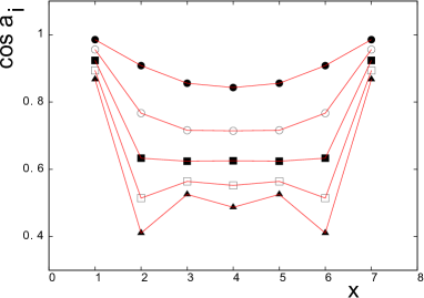
Figure 1: Top: Bulk helical structure along the $c$-axis, in the case $\alpha=2\pi/3$, namely $J_{2}/J_{1}=-2$. Bottom: (color online) Cosinus of $\alpha_{1}=\theta_{1}-\theta_{2}$, …, $\alpha_{7}=\theta_{7}-\theta_{8}$ across the film for $J_{2}/J_{1}=-1.2,-1.4,-1.6,-1.8,-2$ (from top) with $N_{z}=8$: $a_{i}$ stands for $\theta_{i}-\theta_{i+1}$ and $x$ indicates the film layer $i$ where the angle $a_{i}$ with the layer $(i+1)$ is shown. The values of the angles are given in Table I: a strong rearrangement of spins near the surface is observed.

III Green’s function method

Let us define the local spin coordinates as follows: the quantization axis of spin $\vec{S}_{i}$ is on its $\zeta_{i}$ axis which lies in the plane, the $\eta_{i}$ axis of $\vec{S}_{i}$ is along the $c$-axis, and the $\xi_{i}$ axis forms with $\eta_{i}$ and $\zeta_{i}$ axes a direct trihedron. Since the spin configuration is planar, all spins have the same $\eta$ axis. Furthermore, all spins in a given layer are parallel. Let $\hat{\xi}_{i}$, $\hat{\eta}_{i}$ and $\hat{\zeta}_{i}$ be the unit vectors on the local $(\xi_{i},\eta_{i},\zeta_{i})$ axes. We write

$$\vec{S}_{i} = S_{i}^{x}\hat{\xi}_{i}+S_{i}^{y}\hat{\eta}_{i}+S_{i}^{z}\hat{\zeta}_{i}$$ (8)

$$\vec{S}_{j} = S_{j}^{x}\hat{\xi}_{j}+S_{j}^{y}\hat{\eta}_{j}+S_{j}^{z}\hat{\zeta}_{j}$$ (9)

We have (see Fig. 2)

$$\hat{\xi}_{j} = \cos\theta_{ij}\hat{\zeta}_{i}+\sin\theta_{ij}\hat{\xi}_{i}$$

$$\hat{\zeta}_{j} = -\sin\theta_{ij}\hat{\zeta}_{i}+\cos\theta_{ij}\hat{\xi}_{i}$$

$$\hat{\eta}_{j} = \hat{\eta}_{i}$$

where $\cos\theta_{ij}=\cos(\theta_{i}-\theta_{j})$ is the angle between two spins $i$ and $j$. Replacing these into Eq. (9) to express $\vec{S}_{j}$ in the $(\hat{\xi}_{i},\hat{\eta}_{i},\hat{\zeta}_{i})$ coordinates, then calculating $\vec{S}_{i}\cdot\vec{S}_{j}$, we obtain the following exchange Hamiltonian from (1):

$$\mathcal{H}_{e} = -\sum_{<i,j>}J_{i,j}\Bigg{\{}\frac{1}{4}\left(\cos\theta_{ij}-1\right)\left(S^{+}_{i}S^{+}_{j}+S^{-}_{i}S^{-}_{j}\right)$$ (10)

$$+ \frac{1}{4}\left(\cos\theta_{ij}+1\right)\left(S^{+}_{i}S^{-}_{j}+S^{-}_{i}S^{+}_{j}\right)$$

$$+ \frac{1}{2}\sin\theta_{ij}\left(S^{+}_{i}+S^{-}_{i}\right)S^{z}_{j}-\frac{1}{2}\sin\theta_{ij}S^{z}_{i}\left(S^{+}_{j}+S^{-}_{j}\right)$$

$$+ \cos\theta_{ij}S^{z}_{i}S^{z}_{j}\Bigg{\}}$$

At this stage, let us mention that according to the theorem of Mermin and Wagner Mermin continuous isotropic spin models such as XY and Heisenberg spins do not have long-range ordering at finite temperatures in two dimensions. Since we are dealing with the Heisenberg model in a thin film, it is useful to add an anisotropic interaction to create a long-range ordering and a phase transition at finite temperatures. We choose the following anisotropic interaction along the in-plane local spin-quantization axes $z$ of $\mathbf{S}_{i}$ and $\mathbf{S}_{j}$:

$$\mathcal{H}_{a}=-\sum_{<i,j>}I_{i,j}S^{z}_{i}S^{z}_{j}\cos\theta_{ij}$$ (11)

where $I_{i,j}(>0)$ is supposed to be positive, small compared to $J_{1}$, and limited to NN on the $c$-axis. The full Hamiltonian is thus $\mathcal{H}=\mathcal{H}_{e}+\mathcal{H}_{a}$.

Figure 2: Local coordinates in a $xy$-plane perpendicular to the $c$-axis. $Q$ denotes $\theta_{j}-\theta_{i}$.

III.1 General formulation for non collinear magnets

We define the following two double-time Green’s functions in the real space:

$$G_{i,j}(t,t^{\prime}) = <<S_{i}^{+}(t);S_{j}^{-}(t^{\prime})>>$$ (12)

$$= -i\theta(t-t^{\prime})<\left[S_{i}^{+}(t),S_{j}^{-}(t^{\prime})\right]>$$

$$F_{i,j}(t,t^{\prime}) = <<S_{i}^{-}(t);S_{j}^{-}(t^{\prime})>>$$ (13)

$$= -i\theta(t-t^{\prime})<\left[S_{i}^{-}(t),S_{j}^{-}(t^{\prime})\right]>$$

We need these two functions because the equation of motion of the first function generates functions of the second type, and vice-versa. These equations of motion are

$$i\hbar\frac{d}{dt}G_{i,j}\left(t,t^{\prime}\right) = \left<\left[S^{+}_{i}\left(t\right),S^{-}_{j}\left(t^{\prime}\right)\right]\right>\delta\left(t-t^{\prime}\right)$$ (14)

$$- \left<\left<\left[\mathcal{H},S^{+}_{i}\left(t\right)\right];S^{-}_{j}\left(t^{\prime}\right)\right>\right>,$$

$$i\hbar\frac{d}{dt}F_{i,j}\left(t,t^{\prime}\right) = \left<\left[S^{-}_{i}\left(t\right),S^{-}_{j}\left(t^{\prime}\right)\right]\right>\delta\left(t-t^{\prime}\right)$$ (15)

$$- \left<\left<\left[\mathcal{H},S^{-}_{i}\left(t\right)\right];S^{-}_{j}\left(t^{\prime}\right)\right>\right>,$$

Expanding the commutators, and using the Tyablikov decoupling scheme for higher-order functions, for example $<<S_{i^{\prime}}^{z}S_{i}^{+}(t);S_{j}^{-}(t^{\prime})>>\simeq<S_{i^{\prime}}^{z}><<S_{i}^{+}(t);S_{j}^{-}(t^{\prime})>>$ etc., we obtain the following general equations for non collinear magnets:

$$i\hbar\frac{dG_{i,j}(t,t^{\prime})}{dt} = 2<S_{i}^{z}>\delta_{i,j}\delta(t-t^{\prime})$$

$$- \sum_{i^{\prime}}J_{i,i^{\prime}}[<S_{i}^{z}>(\cos\theta_{i,i^{\prime}}-1)\times$$

$$\times F_{i^{\prime},j}(t,t^{\prime})$$

$$+ <S_{i}^{z}>(\cos\theta_{i,i^{\prime}}+1)G_{i^{\prime},j}(t,t^{\prime})$$

$$- 2<S_{i^{\prime}}^{z}>\cos\theta_{i,i^{\prime}}G_{i,j}(t,t^{\prime})]$$

$$+ 2\sum_{i^{\prime}}I_{i,i^{\prime}}<S_{i^{\prime}}^{z}>\cos\theta_{i,i^{\prime}}G_{i,j}(t,t^{\prime})$$

$$i\hbar\frac{dF_{i,j}(t,t^{\prime})}{dt} = \sum_{i^{\prime}}J_{i,i^{\prime}}[<S_{i}^{z}>(\cos\theta_{i,i^{\prime}}-1)\times$$

$$\times G_{i^{\prime},j}(t,t^{\prime})$$

$$+ <S_{i}^{z}>(\cos\theta_{i,i^{\prime}}+1)F_{i^{\prime},j}(t,t^{\prime})$$

$$- 2<S_{i^{\prime}}^{z}>\cos\theta_{i,i^{\prime}}F_{i,j}(t,t^{\prime})]$$

$$- 2\sum_{i^{\prime}}I_{i,i^{\prime}}<S_{i^{\prime}}^{z}>\cos\theta_{i,i^{\prime}}F_{i,j}(t,t^{\prime})$$

III.2 BCC helimagnetic films

In the case of a BCC thin film with a (001) surface, the above equations yield a closed system of coupled equations within the Tyablikov decoupling scheme. For clarity, we separate the sums on NN interactions and NNN interactions as follows:

$$i\hbar\frac{dG_{i,j}(t,t^{\prime})}{dt} = 2<S_{i}^{z}>\delta_{i,j}\delta(t-t^{\prime})$$ (18)

$$- \sum_{k^{\prime}\in NN}J_{i,k^{\prime}}[<S_{i}^{z}>(\cos\theta_{i,k^{\prime}}-1)\times$$

$$\times F_{k^{\prime},j}(t,t^{\prime})$$

$$+ <S_{i}^{z}>(\cos\theta_{i,k^{\prime}}+1)G_{k^{\prime},j}(t,t^{\prime})$$

$$- 2<S_{k^{\prime}}^{z}>\cos\theta_{i,k^{\prime}}G_{i,j}(t,t^{\prime})]$$

$$+ 2\sum_{k^{\prime}\in NN}I_{i,k^{\prime}}<S_{k^{\prime}}^{z}>\cos\theta_{i,k^{\prime}}G_{i,j}(t,t^{\prime})$$

$$- \sum_{i^{\prime}\in NNN}J_{i,i^{\prime}}[<S_{i}^{z}>(\cos\theta_{i,i^{\prime}}-1)\times$$

$$\times F_{i^{\prime},j}(t,t^{\prime})$$

$$+ <S_{i}^{z}>(\cos\theta_{i,i^{\prime}}+1)G_{i^{\prime},j}(t,t^{\prime})$$

$$- 2<S_{i^{\prime}}^{z}>\cos\theta_{i,i^{\prime}}G_{i,j}(t,t^{\prime})]$$

$$i\hbar\frac{dF_{k,j}(t,t^{\prime})}{dt} = \sum_{i^{\prime}\in NN}J_{k,i^{\prime}}[<S_{k}^{z}>(\cos\theta_{k,i^{\prime}}-1)\times$$ (19)

$$\times G_{i^{\prime},j}(t,t^{\prime})$$

$$+ <S_{k}^{z}>(\cos\theta_{k,i^{\prime}}+1)F_{i^{\prime},j}(t,t^{\prime})$$

$$- 2<S_{i^{\prime}}^{z}>\cos\theta_{k,i^{\prime}}F_{k,j}(t,t^{\prime})]$$

$$- 2\sum_{i^{\prime}\in NN}I_{k,i^{\prime}}<S_{i^{\prime}}^{z}>\cos\theta_{k,i^{\prime}}F_{k,j}(t,t^{\prime})$$

$$+ \sum_{k^{\prime}\in NNN}J_{k,k^{\prime}}[<S_{k}^{z}>(\cos\theta_{k,k^{\prime}}-1)\times$$

$$\times G_{k^{\prime},j}(t,t^{\prime})$$

$$+ <S_{k}^{z}>(\cos\theta_{k,k^{\prime}}+1)F_{k^{\prime},j}(t,t^{\prime})$$

$$- 2<S_{k^{\prime}}^{z}>\cos\theta_{k,k^{\prime}}F_{k,j}(t,t^{\prime})]$$

For simplicity, except otherwise stated, all NN interactions $(J_{k,k^{\prime}},I_{k,k^{\prime}})$ are taken equal to $(J_{1},I_{1})$ and all NNN interactions are taken equal to $J_{2}$ in the following. Furthermore, let us define the film coordinates which are used below: the $c$-axis is called $z$-axis, planes parallel to the film surface are called $xy$-planes and the Cartesian components of the spin position $\mathbf{R}_{i}$ are denoted by $(\ell_{i},m_{i},n_{i})$.

We now introduce the following in-plane Fourier transforms:

$$G_{i,j}\left(t,t^{\prime}\right) = \frac{1}{\Delta}\int\int_{BZ}d\mathbf{k}_{xy}\frac{1}{2\pi}\int^{+\infty}_{-\infty}d\omega e^{-i\omega\left(t-t^{\prime}\right)}$$ (20)

$$\hskip 19.91684pt\times g_{n_{i},n_{j}}\left(\omega,\mathbf{k}_{xy}\right)e^{i\mathbf{k}_{xy}\cdot\left(\mathbf{R}_{i}-\mathbf{R}_{j}\right)},$$

$$F_{k,j}\left(t,t^{\prime}\right) = \frac{1}{\Delta}\int\int_{BZ}d\mathbf{k}_{xy}\frac{1}{2\pi}\int^{+\infty}_{-\infty}d\omega e^{-i\omega\left(t-t^{\prime}\right)}$$ (21)

$$\hskip 19.91684pt\times f_{n_{k},n_{j}}\left(\omega,\mathbf{k}_{xy}\right)e^{i\mathbf{k}_{xy}\cdot\left(\mathbf{R}_{k}-\mathbf{R}_{j}\right)},$$

where $\omega$ is the spin-wave frequency, $\mathbf{k}_{xy}$ denotes the wave-vector parallel to $xy$ planes and $\mathbf{R}_{i}$ is the position of the spin at the site $i$. $n_{i}$, $n_{j}$ and $n_{k}$ are respectively the $z$-component indices of the layers where the sites $\mathbf{R}_{i}$, $\mathbf{R}_{j}$ and $\mathbf{R}_{k}$ belong to. The integral over $\mathbf{k}_{xy}$ is performed in the first Brillouin zone ($BZ$) whose surface is $\Delta$ in the $xy$ reciprocal plane. For convenience, we denote $n_{i}=1$ for all sites on the surface layer, $n_{i}=2$ for all sites of the second layer and so on.

Note that for a three-dimensional case, making a 3D Fourier transformation of Eqs. (18)-(19) we obtain the spin-wave dispersion relation in the absence of anisotropy:

$$\hbar\omega=\pm\sqrt{A^{2}-B^{2}}$$ (22)

where

$$A = J_{1}\left<S^{z}\right>[\cos\theta+1]Z\gamma+2ZJ_{1}\left<S^{z}\right>\cos\theta$$

$$+J_{2}\left<S^{z}\right>[\cos(2\theta)+1]Z_{c}\cos(k_{z}a)$$

$$+2Z_{c}J_{2}\left<S^{z}\right>\cos(2\theta)$$

$$B = J_{1}\left<S^{z}\right>(\cos\theta-1)Z\gamma$$

$$+J_{2}\left<S^{z}\right>[\cos(2\theta)-1]Z_{c}\cos(k_{z}a)$$

where $Z=8$ (NN number), $Z_{c}=2$ (NNN number on the $c$-axis), $\gamma=\cos(k_{x}a/2)\cos(k_{y}a/2)\cos(k_{z}a/2)$ ($a$: lattice constant). We see that $\hbar\omega$ is zero when $A=\pm B$, namely at $k_{x}=k_{y}=k_{z}=0$ ($\gamma=1$) and at $k_{z}=2\theta$ along the helical axis. The case of ferromagnets (antiferromagnets) with NN interaction only is recovered by putting $\cos\theta=1$ $(-1)$ Diep1979 .

Let us return to the film case. We make the in-plane Fourier transformation Eqs. (20)-(21) for Eqs. (18)-(19). We obtain the following matrix equation

$$\mathbf{M}\left(\omega\right)\mathbf{h}=\mathbf{u},$$ (23)

where $\mathbf{M}\left(\omega\right)$ is a square matrix of dimension $\left(2N_{z}\times 2N_{z}\right)$, $\mathbf{h}$ and $\mathbf{u}$ are the column matrices which are defined as follows

$$\mathbf{h}=\left(\begin{array}[]{c}g_{1,n^{\prime}}\\ f_{1,n^{\prime}}\\ \vdots\\ g_{n,n^{\prime}}\\ f_{n,n^{\prime}}\\ \vdots\\ g_{N_{z},n^{\prime}}\\ f_{N_{z},n^{\prime}}\\ \end{array}\right),\mathbf{u}=\left(\begin{array}[]{c}2\left<S^{z}_{1}\right>\delta_{1,n^{\prime}}\\ 0\\ \vdots\\ 2\left<S^{z}_{N_{z}}\right>\delta_{N_{z},n^{\prime}}\\ 0\\ \end{array}\right),$$ (24)

where, taking $\hbar=1$ hereafter,

$$\mathbf{M}\left(\omega\right)=\left(\begin{array}[]{cccccccccccc}\omega+A_{1}&0&B^{+}_{1}&C^{+}_{1}&D_{1}^{+}&E_{1}^{+}&0&0&0&0&0&0\\ 0&\omega-A_{1}&-C^{+}_{1}&-B^{+}_{1}&-E_{1}^{+}&-D_{1}^{+}&0&0&0&0&0&0\\ \cdots&\cdots&\cdots&\cdots&\cdots&\cdots&\cdots&\cdots&\cdots&\cdots&\cdots&\cdots\\ \cdots&D_{n}^{-}&E_{n}^{-}&B^{-}_{n}&C^{-}_{n}&\omega+A_{n}&0&B^{+}_{n}&C^{+}_{n}&D_{n}^{+}&E_{n}^{+}&\cdots\\ \cdots&-E_{n}^{-}&-D_{n}^{-}&-C^{-}_{n}&-B^{-}_{n}&0&\omega-A_{n}&-C^{+}_{n}&-B^{+}_{n}&-E_{n}^{+}&-D_{n}^{+}&\cdots\\ \cdots&\cdots&\cdots&\cdots&\cdots&\cdots&\cdots&\cdots&\cdots&\cdots&\cdots&\cdots\\ 0&0&0&0&0&0&D^{-}_{N_{z}}&E^{-}_{N_{z}}&B^{-}_{N_{z}}&C^{-}_{N_{z}}&\omega+A_{N_{z}}&0\\ 0&0&0&0&0&0&-E^{-}_{N_{z}}&-D^{-}_{N_{z}}&-C^{-}_{N_{z}}&-B^{-}_{N_{z}}&0&\omega-A_{N_{z}}\\ \end{array}\right)$$ (25)

where

$$A_{n} = -8J_{1}(1+d)\Big{[}\left<S^{z}_{n+1}\right>\cos\theta_{n,n+1}$$

$$+\left<S^{z}_{n-1}\right>\cos\theta_{n,n-1}\Big{]}$$

$$- 2J_{2}\Big{[}\left<S^{z}_{n+2}\right>\cos\theta_{n,n+2}$$

$$+\left<S^{z}_{n-2}\right>\cos\theta_{n,n-2}\Big{]}$$

where $n=1,2,...,N_{z}$, $d=I_{1}/J_{1}$, and

$$B_{n}^{\pm} = 4J_{1}\left<S^{z}_{n}\right>(\cos\theta_{n,n\pm 1}+1)\gamma$$

$$C_{n}^{\pm} = 4J_{1}\left<S^{z}_{n}\right>(\cos\theta_{n,n\pm 1}-1)\gamma$$

$$E_{n}^{\pm} = J_{2}\left<S^{z}_{n}\right>(\cos\theta_{n,n\pm 2}-1)$$

$$D_{n}^{\pm} = J_{2}\left<S^{z}_{n}\right>(\cos\theta_{n,n\pm 2}+1)$$

In the above expressions, $\theta_{n,n\pm 1}$ the angle between a spin in the layer $n$ and its NN spins in layers $n\pm 1$ etc. and $\gamma=\cos\left(\frac{k_{x}a}{2}\right)\cos\left(\frac{k_{y}a}{2}\right).$

Solving det$|\mathbf{M}|=0$, we obtain the spin-wave spectrum $\omega$ of the present system: for each value ($k_{x},k_{y})$, there are 2$N_{z}$ eigen-values of $\omega$ corresponding to two opposite spin precessions as in antiferromagnets (the dimension of det$|\mathbf{M}|$ is $2N_{z}\times 2N_{z}$). Note that the above equation depends on the values of $<S_{n}^{z}>$ ($n=1,...,N_{z}$). Even at temperature $T=0$, these $z$-components are not equal to $1/2$ because we are dealing with an antiferromagnetic system where fluctuations at $T=0$ give rise to the so-called zero-point spin contraction DiepTM . Worse, in our system with the existence of the film surfaces, the spin contractions are not spatially uniform as will be seen below. So the solution of det$|\mathbf{M}|=0$ should be found by iteration. This will be explicitly shown hereafter.

The solution for $g_{n,n}$ is given by

$$g_{n,n}(\omega)=\frac{\left|\mathbf{M}\right|_{2n-1}}{\left|\mathbf{M}\right|},$$ (26)

where $\left|\mathbf{M}\right|_{2n-1}$ is the determinant made by replacing the $2n-1$-th column of $\left|\mathbf{M}\right|$ by $\mathbf{u}$ given by Eq. (24) [note that $g_{n,n}$ occupies the $(2n-1)$-th line of the matrix $\mathbf{h}$]. Writing now

$$\left|\mathbf{M}\right|=\prod_{i}\left[\omega-\omega_{i}\left(\mathbf{k}_{xy}\right)\right],$$ (27)

we see that $\omega_{i}\left(\mathbf{k}_{xy}\right),\ i=1,\cdots,\ 2N_{z}$, are poles of $g_{n,n}$. $\omega_{i}\left(\mathbf{k}_{xy}\right)$ can be obtained by solving $\left|\mathbf{M}\right|=0$. In this case, $g_{n,n}$ can be expressed as

$$g_{n,n}(\omega)=\sum_{i}\frac{D_{2n-1}\left(\omega_{i}\left(\mathbf{k}_{xy}\right)\right)}{\left[\omega-\omega_{i}\left(\mathbf{k}_{xy}\right)\right]},$$ (28)

where $D_{2n-1}\left(\omega_{i}\left(\mathbf{k}_{xy}\right)\right)$ is

$$D_{2n-1}\left(\omega_{i}\left(\mathbf{k}_{xy}\right)\right)=\frac{\left|\mathbf{M}\right|_{2n-1}\left(\omega_{i}\left(\mathbf{k}_{xy}\right)\right)}{\prod_{j\neq i}\left[\omega_{j}\left(\mathbf{k}_{xy}\right)-\omega_{i}\left(\mathbf{k}_{xy}\right)\right]}.$$ (29)

Next, using the spectral theorem which relates the correlation function $\langle S^{-}_{i}S^{+}_{j}\rangle$ to the Green’s function zu , we have

$$\left<S^{-}_{i}S^{+}_{j}\right> = \lim_{\varepsilon\rightarrow 0}\frac{1}{\Delta}\int\int d\mathbf{k}_{xy}\int^{+\infty}_{-\infty}\frac{i}{2\pi}\big{(}g_{n,n^{\prime}}\left(\omega+i\varepsilon\right)$$ (30)

$$- g_{n,n^{\prime}}\left(\omega-i\varepsilon\right)\big{)}\frac{d\omega}{e^{\beta\omega}-1}e^{i\mathbf{k}_{xy}\cdot\left(\mathbf{R}_{i}-\mathbf{R}_{j}\right)},$$

where $\epsilon$ is an infinitesimal positive constant and $\beta=(k_{B}T)^{-1}$, $k_{B}$ being the Boltzmann constant.

Using the Green’s function presented above, we can calculate self-consistently various physical quantities as functions of temperature $T$. The magnetization $\langle S_{n}^{z}\rangle$ of the $n$-th layer is given by

$$\langle S_{n}^{z}\rangle = \frac{1}{2}-\left<S^{-}_{n}S^{+}_{n}\right>$$ (31)

$$= \frac{1}{2}-\lim_{\epsilon\to 0}\frac{1}{\Delta}\int\int d{\bf k_{xy}}\int\limits_{-\infty}^{+\infty}\frac{i}{2\pi}[g_{n,n}(\omega+i\epsilon)$$

$$-g_{n,n}(\omega-i\epsilon)]\frac{d\omega}{\mbox{e}^{\beta\omega}-1}$$

Replacing Eq. (28) in Eq. (31) and making use of the following identity

$$\frac{1}{x-i\eta}-\frac{1}{x+i\eta}=2\pi i\delta(x)$$ (32)

we obtain

$$\langle S_{n}^{z}\rangle=\frac{1}{2}-\frac{1}{\Delta}\int\int dk_{x}dk_{y}\sum_{i=1}^{2N_{z}}\frac{D_{2n-1}(\omega_{i})}{\mbox{e}^{\beta\omega_{i}}-1}$$ (33)

where $n=1,...,N_{z}$. As $<S_{n}^{z}>$ depends on the magnetizations of the neighboring layers via $\omega_{i}(i=1,...,2N_{z})$, we should solve by iteration the equations (33) written for all layers, namely for $n=1,...,N_{z}$, to obtain the magnetizations of layers 1, 2, 3, …, $N_{z}$ at a given temperature $T$. Note that by symmetry, $<S_{1}^{z}>=<S_{N_{z}}^{z}>$, $<S_{2}^{z}>=<S_{N_{z}-1}^{z}>$, $<S_{3}^{z}>=<S_{N_{z}-2}^{z}>$, and so on. Thus, only $N_{z}/2$ self-consistent layer magnetizations are to be calculated.

The value of the spin in the layer $n$ at $T=0$ is calculated by

$$\langle S_{n}^{z}\rangle(T=0)=\frac{1}{2}+\frac{1}{\Delta}\int\int dk_{x}dk_{y}\sum_{i=1}^{N_{z}}D_{2n-1}(\omega_{i})$$ (34)

where the sum is performed over $N_{z}$ negative values of $\omega_{i}$ (for positive values the Bose-Einstein factor is equal to 0 at $T=0$).

The transition temperature $T_{c}$ can be calculated in a self-consistent manner by iteration, letting all $<S_{n}^{z}>$ tend to zero, namely $\omega_{i}\rightarrow 0$. Expanding $\mbox{e}^{\beta\omega_{i}}-1\rightarrow\beta_{c}\omega_{i}$ on the right-hand side of Eq. (33) where $\beta_{c}=(k_{B}T_{c})^{-1}$, we have by putting $\langle S_{n}^{z}\rangle=0$ on the left-hand side,

$$\beta_{c}=2\frac{1}{\Delta}\int\int dk_{x}dk_{y}\sum_{i=1}^{2N_{z}}\frac{D_{2n-1}(\omega_{i})}{\omega_{i}}$$ (35)

There are $N_{z}$ such equations using Eq. (33) with $n=1,...,N_{z}$. Since the layer magnetizations tend to zero at the transition temperature from different values, it is obvious that we have to look for a convergence of the solutions of the equations Eq. (35) to a single value of $T_{c}$. The method to do this will be shown below.

IV Results from the Green’s function method

Let us take $J_{1}=1$, namely ferromagnetic interaction between NN. We consider the helimagnetic case where the NNN interaction $J_{2}$ is negative and $|J_{2}|>J_{1}$. The non uniform GS spin configuration across the film has been determined in section II for each value of $p=J_{2}/J_{1}$. Using the values of $\theta_{n,n\pm 1}$ and $\theta_{n,n\pm 2}$ to calculate the matrix elements of $\left|\mathbf{M}\right|$, then solving det$\left|\mathbf{M}\right|=0$ we find the eigenvalues $\omega_{i}(i=1,...,2N_{z})$ for each $\mathbf{k}_{xy}$ with a input set of $\langle S_{n}^{z}\rangle(n=1,...,N_{z})$ at a given $T$. Using Eq. (33) for $n=1,...,N_{z}$ we calculate the output $\langle S_{n}^{z}\rangle(n=1,...,N_{z})$. Using this output set as input, we calculate again $\langle S_{n}^{z}\rangle(n=1,...,N_{z})$ until the input and output are identical within a desired precision $P$. Numerically, we use a Brillouin zone of $100^{2}$ wave-vector values, and we use the obtained values $\langle S_{n}^{z}\rangle$ at a given $T$ as input for a neighboring $T$. At low $T$ and up to $\sim\frac{4}{5}T_{c}$, only a few iterations suffice to get $P\leq 1\%$. Near $T_{c}$, several dozens of iteration are needed to get convergence. We show below our results.

IV.1 Spectrum

We calculated the spin-wave spectrum as described above for each a given $J_{2}/J_{1}$. The spin-wave spectrum depends on the temperature via the temperature-dependence of layer magnetizations. Let us show in Fig. 3 the spin-wave frequency $\omega$ versus $k_{x}=k_{y}$ in the case on an 8-layer film where $J_{2}/J_{1}=-1.4$ at two temperatures $T=0.1$ and $T=1.02$ (in units of $J_{1}/k_{B}=1$). There are 8 positive and 8 negative modes corresponding two opposite spin precessions. Note that there are two degenerate acoustic surface branches lying at low energy on each side. This degeneracy comes from the two symmetrical surfaces of the film. These surface modes propagate parallel to the film surface but are damped from the surface inward. As $T$ increases, layer magnetizations decrease (see below), reducing therefore the spin-wave energy as seen in Fig. 3 (bottom).

Figure 3: Spectrum $E=\hbar\omega$ versus $k\equiv k_{x}=k_{y}$ for $J_{2}/J_{1}=-1.4$ at $T=0.1$ (top) and $T=1.02$ (bottom) for $N_{z}=8$ and $d=0.1$. The surface branches are indicated by $s$.

IV.2 Spin contraction at $T=0$ and transition temperature

It is known that in antiferromagnets, quantum fluctuations give rise to a contraction of the spin length at zero temperature DiepTM . We will see here that a spin under a stronger antiferromagnetic interaction has a stronger zero-point spin contraction. The spins near the surface serve for such a test. In the case of the film considered above, spins in the first and in the second layers have only one antiferromagnetic NNN while interior spins have two NNN, so the contraction at a given $J_{2}/J_{1}$ is expected to be stronger for interior spins. This is verified with the results shown in Fig. 4. When $|J_{2}|/J_{1}$ increases, namely the antiferromagnetic interaction becomes stronger, we observe stronger contractions. Note that the contraction tends to zero when the spin configuration becomes ferromagnetic, namely $J_{2}$ tends to -1.

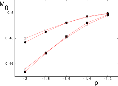
Figure 4: (Color online) Spin lengths of the first four layers at $T=0$ for several values of $p=J_{2}/J_{1}$ with $d=0.1$, $N_{z}=8$. Black circles, void circles, black squares and void squares are for first, second, third and fourth layers, respectively. See text for comments.

IV.3 Layer magnetizations

Let us show two examples of the magnetization, layer by layer, from the film surface in Figs. 5 and 6, for the case where $J_{2}/J_{1}=-1.4$ and -2 in a $N_{z}=8$ film. Let us comment on the case $J_{2}/J_{1}=-1.4$:

(i) the shown result is obtained with a convergence of $1\%$. For temperatures closer to the transition temperature $T_{c}$, we have to lower the precision to a few percents which reduces the clarity because of their close values (not shown).

(ii) the surface magnetization, which has a large value at $T=0$ as seen in Fig. 4, crosses the interior layer magnetizations at $T\simeq 0.42$ to become much smaller than interior magnetizations at higher temperatures. This crossover phenomenon is due to the competition between quantum fluctuations, which dominate low-$T$ behavior, and the low-lying surface spin-wave modes which strongly diminish the surface magnetization at higher $T$. Note that the second-layer magnetization makes also a crossover at $T\simeq 1.3$. Similar crossovers have been observed in quantum antiferromagnetic films DiepTF91 and quantum superlattices DiepSL89 .

Similar remarks can be also made for the case $J_{2}/J_{1}=-2$.

Note that though the layer magnetizations are different at low temperatures, they will tend to zero at a unique transition temperature as seen below. The reason is that as long as an interior layer magnetization is not zero, it will act on the surface spins as an external field, preventing them to become zero.

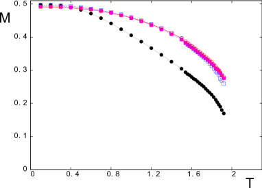
Figure 5: (Color online) Layer magnetizations as functions of $T$ for $J_{2}/J_{1}=-1.4$ with $d=0.1$, $N_{z}=8$ (top). Zoom of the region at low $T$ to show crossover (bottom). Black circles, blue void squares, magenta squares and red void circles are for first, second, third and fourth layers, respectively. See text.

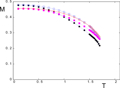
Figure 6: (Color online) Layer magnetizations as functions of $T$ for $J_{2}/J_{1}=-2$ with $d=0.1$, $N_{z}=8$ (top). Zoom of the region at low $T$ to show crossover (bottom). Black circles, blue void squares, magenta squares and red void circles are for first, second, third and fourth layers, respectively. See text.

The temperature where layer magnetizations tend to zero is calculated by Eq. (35). Since all layer magnetizations tend to zero from different values, we have to solve self-consistently $N_{z}$ equations (35) to obtain the transition temperature $T_{c}$. One way to do it is to use the self-consistent layer magnetizations obtained as described above at a temperature as close as possible to $T_{c}$ as input for Eq. (35). As long as the $T$ is far from $T_{c}$ the convergence is not reached: we have four ’pseudo-transition temperatures’ $T_{cs}$ as seen in Fig. 7, one for each layer. The convergence of these $T_{cs}$ can be obtained by a short extrapolation from temperatures when they are rather close to each other. $T_{c}$ is thus obtained with a very small extrapolation error as seen in Fig. 7 for $p=J_{2}/J_{1}=-1.4$: $T_{c}\simeq 2.313\pm 0.010$. The results for several $p=J_{2}/J_{1}$ are shown in Fig. 8.

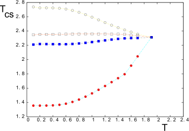
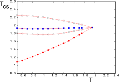
Figure 7: (Color online) Top: Transition temperature is calculated at $p=J_{2}/J_{1}=-1.4$ for $d=0.1$, $N_{z}=8$: at each temperature, using the self-consistent values of layer magnetizations at $T<T_{c}$, Eq.(35) is solved to obtain $T_{cs}$ for each layer. The convergence is reached when $T_{cs}$ tend to a single value $T_{c}$. One has $T_{c}\simeq 2.313\pm 0.010$. Red circles, black void circles, blue squares and blue void squares are $T_{cs}$ obtained from Eq. (35) for first, second, third and fourth layers, respectively, at different temperatures. Bottom: Extrapolation by lines to obtain $T_{c}$ is shown for surface parameter $J_{1}^{s}/J_{1}=0.7$. The precision for self-consistent convergence is $1\%$ for layer magnetizations. See text for comments.

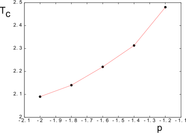
Figure 8: (Color online) Transition temperature versus $p=J_{2}/J_{1}$ for an 8-layer film with $d=0.1$. See text for comments.

IV.4 Effect of anisotropy and surface parameters

The results shown above have been calculated with an in-plane anisotropy interaction $d=0.1$. Let us show now the effect of $d$. Stronger $d$ will enhance all the layer magnetizations and increase $T_{c}$. Figure 9 shows the surface magnetization versus $T$ for several values of $d$ (other layer magnetizations are not shown to preserve the figure clarity).

Figure 9: Surface magnetization versus $T$ for $d=0.05$ (circles), 0.1 (void circles), 0.2 (squares), 0.3 (void squares) and 0.4 (triangles), with $J_{2}/J_{1}=-1.4$, $N_{z}=16$.

The transition temperatures are $2.091\pm 0.010$, $2.313\pm 0.010$, $2.752\pm 0.010$, $3.195\pm 0.010$ and $3.630\pm 0.010$ for $d=0.05$, 0.1, 0.2, 0.3 and 0.4, respectively. These values versus $d$ lie on a remarkable straight line.

Let us examine the effects of the surface anisotropy and exchange parameters $d_{s}$ and $J_{1}^{s}$. As seen above, even in the case where the surface interaction parameters are the same as those in the bulk the surface spin-wave modes exist in the spectrum. These localized modes cause a low surface magnetization observed in Figs. 5 and 6. Here, we show that with a weaker NN exchange interaction between surface spins and the second-layer ones, namely $J_{1}^{s}<J_{1}$, the surface magnetization becomes even much smaller with respect to the magnetizations of interior layers. This is shown in Fig. 10 for several values of $J_{1}^{s}$. We observe again here the crossover of layer magnetizations at low $T$ due to quantum fluctuations as discussed earlier. The transition temperature strongly decreases with $J_{1}^{s}$: we have $T_{c}=2.103\pm 0.010$, $1.951\pm 0.010$, $1.880\pm 0.010$ and $1.841\pm 0.010$ for $J_{1}^{s}=1$, 0.7, 0.5 and 0.3, respectively ($N_{z}=16$, $J_{2}/J_{1}=-2$, $d=d_{s}=0.1$). Note that the value $J_{1}^{s}=0.5$ is a very particular value: the GS configuration is a uniform configuration with all angles equal to $60^{\circ}$, namely there is no surface spin rearrangement. This can be explained if we look at the local field acting on the surface spins: the lack of neighbors is compensated by this weak positive value of $J_{1}^{s}$ so that their local field is equal to that of a bulk spin. There is thus no surface reconstruction. Nevertheless, as $T$ increases, thermal effects will strongly diminish the surface magnetization as seen in Fig. 10 (middle). As for the surface anisotropy parameter $d_{s}$, it affects strongly the layer magnetizations and the transition temperature: we show in Fig. 11 the surface magnetizations and the transition temperature for several values of $d_{s}$.

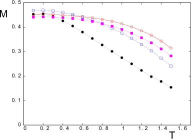
Figure 10: (Color online) Layer magnetizations as functions of $T$ for the surface interaction $J_{1}^{s}=0.3$ (top), 0.5 (middle) and 0.7 (bottom) with $J_{2}/J_{1}=-2$, $d=0.1$ and $N_{z}=16$. Black circles, blue void squares, magenta squares and red void circles are for first, second, third and fourth layers, respectively.

Figure 11: Top: Surface magnetization versus $T$ for $d_{s}=0.01$ (circles), 0.1 (void circles), 0.2 (squares) and 0.3 (void squares), with $J_{1}^{s}=1$, $J_{2}/J_{1}=-2$ and $N_{z}=16$. Bottom: Transition temperature versus $d_{s}$ for $J_{1}^{s}$=0.7, 0.5 and 0.3 (curves from up to down), with $J_{2}/J_{1}=-2$, $d=0.1$ and $N_{z}=16$.

IV.5 Effect of the film thickness

We have performed calculations for $N_{z}=8$, 12 and 16. The results show that the effect of the thickness at these values is not significant: the difference lies within convergence errors. Note that the classical ground state of the first four layers is almost the same: for example, here are the values of cosinus of the angles of the film first half for $N_{z}=16$ which are to be compared with the values for $N_{z}=8$ given in Table I, for $p=J_{2}/J_{1}=-2$ (in parentheses are angles in degree):

0.86737967 (29.844446), 0.41125694 (65.716179), 0.52374715 (58.416061), 0.49363765 (60.420044), 0.50170541 (59.887100), 0.49954081 (60.030373), 0.50013113 (59.991325), 0.49993441 (60.004330).

From the 4th layer, the angle is almost equal to the bulk value ($60^{\circ}$).

At $p=J_{2}/J_{1}=-2$, the transition temperature is $2.090\pm 0.010$ for $N_{z}=8$, $2.093\pm 0.010$ for $N_{z}=12$ and $2.103\pm 0.010$ for $N_{z}=16$. These are the same within errors. At smaller thicknesses, the difference can be seen. However, for helimagnets in the $z$ direction, thicknesses smaller than 8 do not allow to see fully the surface helical reconstruction which covers the first four layers: to study surface helical effects in such a situation would not make sense.

At this stage, it is interesting to note that our result is in excellent agreement with experiments: it has been experimentally observed that the transition temperature does not vary significantly in MnSi films in the thickness range of $11-40$ nm Karhu2011 . One possible explanation is that the helical structure is very stable as seen above: the surface perturbs the bulk helical configuration only at the first four layers, so the bulk ’rigidity’ dominates the transition. This has been experimentally seen in holmium films Leiner .

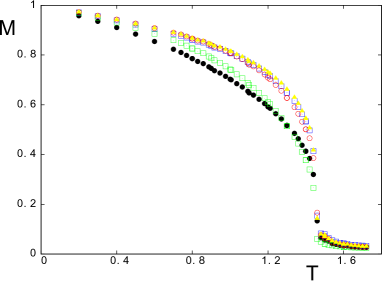
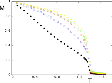
Figure 12: (Color online) Monte Carlo results: Layer magnetizations as functions of $T$ for the surface interaction $J_{1}^{s}=1$ (top) and 0.3 (bottom) with $J_{2}/J_{1}=-2$ and $N_{z}=16$. Black circles, blue void squares, cyan squares and red void circles are for first, second, third and fourth layers, respectively.

IV.6 Classical helimagnetic films: Monte Carlo simulation

To appreciate quantum effects causing crossovers of layer magnetizations presented above at low temperatures, we show here some results of the classical counterpart model: spins are classical XY spins of amplitude $S=1$. We take the XY spins rather than the Heisenberg spins for comparison with the quantum case because in the latter case we have used an in-plane Ising-like anisotropy interaction $d$. Monte Carlo simulations have been carried out over film samples of $100\times 100\times 16$. Periodic boundary conditions are applied in the $xy$ plane. One million of MC steps are discarded to equilibrate the system and another million of MC steps are used for averaging. The layer magnetizations versus $T$ are shown in Fig. 12 for the case where surface interaction $J_{1}^{s}=1$ (top) and 0.3 (bottom) with $J_{2}/J_{1}=-2$ and $N_{z}=16$. One sees that i) by extrapolation there is no spin contraction at $T=0$ and there is no crossover of layer magnetizations at low temperatures, ii) from the intermediate temperature region up to the transition the relative values of layer magnetizations are not always the same as in the quantum case: for example at $T=1.2$, one has $M_{1}<M_{3}<M_{4}<M_{2}$ in Fig. 12 (top) and $M_{1}<M_{2}<M_{4}<M_{3}$ in Fig. 12 (bottom) which are not the same as in the quantum case shown in Fig. 6 (top) and Fig. 10 (top). Our conclusion is that even at temperatures close to the transition, helimagnets may have slightly different behaviors according to their quantum or classical nature. Extensive MC simulations with size effects and detection of the order of the phase transition is not the scope of this present paper.

V Conclusion

We have studied in this paper surface effects in a helimagnet of body-centered cubic lattice with quantum Heisenberg spins. The classical bulk ground-state spin configuration is exactly calculated and is found to be strongly modified near the film surface. The surface spin rearrangement is however limited to the first four layers in our model, regardless of the bulk angle, namely the NNN interaction strength $J_{2}$. The spin-wave excitation is calculated using a general Green’s function technique for non collinear spin configurations. The layer magnetization as a function of temperature as well as the transition temperature are shown for various interaction parameters. Among the striking features found in the present paper, let us mention i) the cross-over of layer magnetizations at low temperatures due to the competition between quantum fluctuations and thermal effects, ii) the existence of low-lying surface spin-wave modes which cause a low surface magnetization, iii) a strong effect of the surface exchange interaction ($J_{1}^{s}$) which drastically modifies the surface spin configuration and gives rise to a very low surface magnetization, iv) the transition temperature varies strongly with the helical angle but it is insensitive to the film thickness in agreement with experiments performed on MnSi films Karhu2011 and holmium Leiner , v) the classical spin model counterpart gives features slightly different from those of the quantum model, both at low and high temperatures.

To conclude, let us emphasize that the general theoretical method proposed here allows us to study at a microscopic level surface spin-waves and their physical consequences at finite temperatures in systems with non collinear spin configurations such as helimagnetic films. It can be used in more complicated situations such as helimagnets with Dzyaloshinskii-Moriya interactions Karhu2012 .

References

• (1) A. Yoshimori, J. Phys. Soc. Jpn 14, 807 (1959).
• (2) J. Villain, Phys. Chem. Solids 11, 303 (1959).
• (3) I. Harada and K. Motizuki, J. Phys. Soc. Jpn 32, 927 (1972).
• (4) E. Rastelli, L. Reatto and A. Tassi, Quantum fluctuations in helimagnets, J. Phys. C 18, 353 (1985).
• (5) H. T. Diep, Low-temperature properties of quantum Heisenberg helimagnets, Phys. Rev. B 40, 741 (1989).
• (6) R. Quartu and H. T. Diep, Phase diagram of body-centered tetragonal Helimagnets, J. Magn. Magn. Mater. 182, 38 (1998).
• (7) S. M. Stishov, A. E. Petrova, S. Khasanov, G. Kh. Panova, A. A. Shikov, J. C. Lashley, D. Wu, and T. A. Lograsso, Magnetic phase transition in the itinerant helimagnet MnSi: Thermodynamic and transport properties, Phys. Rev. B 76, 052405 (2007).
• (8) H. T. Diep, Magnetic transitions in helimagnets, Phys. Rev. B 39, 397 (1989).
• (9) V. Thanh Ngo and H. T. Diep, Stacked triangular XY antiferromagnets: End of a controversial issue on the phase transition, J. Appl. Phys. 103, 07C712 (2007).
• (10) V. Thanh Ngo and H. T. Diep, Phase transition in Heisenberg stacked triangular antiferromagnets: End of a controversy, Phys. Rev. E 78, 031119 (2008).
• (11) H. T. Diep (ed.), Frustrated Spin Systems, 2nd edition, World Scientific (2013).
• (12) Ultrathin Magnetic Structures, vol. I and II, J.A.C. Bland and B. Heinrich (editors), Springer-Verlag (1994).
• (13) A. Zangwill, Physics at Surfaces, Cambridge University Press (1988).
• (14) V. D. Mello, C. V. Chianca, Ana L. Danta, and A. S. Carriç, Magnetic surface phase of thin helimagnetic films, Phys. Rev. B 67, 012401 (2003).
• (15) F. Cinti, A. Cuccoli, and A. Rettori, Exotic magnetic structures in ultrathin helimagnetic holmium films, Phys. Rev. B 78, 020402(R) (2008).
• (16) E. A. Karhu, S. Kahwaji, M. D. Robertson, H. Fritzsche, B. J. Kirby, C. F. Majkrzak, and T. L. Monchesky, Helical magnetic order in MnSi thin films, Phys. Rev. B 84, 060404(R) (2011).
• (17) E. A. Karhu, U. K. Rö$\beta$ler, A. N. Bogdanov, S. Kahwaji, B. J. Kirby, H. Fritzsche, M. D. Robertson, C. F. Majkrzak, and T. L. Monchesky, Chiral modulation and reorientation effects in MnSi thin films, Phys. Rev. B 85, 094429 (2012).
• (18) J. Heurich, J. König, and A. H. MacDonald, Phys. Rev. B 68, 064406 (2003).
• (19) O. Wessely, B. Skubic, and L. Nordstrom, Phys. Rev. B 79, 104433 (2009).
• (20) F. Jonietz, S. Mühlbauer, C. Pfleiderer, A. Neubauer, W. Munzer, A. Bauer, T. Adams, R. Georgii, P. Böni, R. A. Duine, K. Everschor, M. Garst, and A. Risch, Science 330, 1648 (2010).
• (21) D. N. Zubarev, Usp. Fiz. Nauk 187, 71 (1960)[translation: Soviet Phys.-Uspekhi 3, 320 (1960)].
• (22) Diep-The-Hung, J. C. S. Levy and O. Nagai, Effect of surface spin-waves and surface anisotropy in magnetic thin films at finite temperatures, Phys. Stat. Solidi (b) 93, 351 (1979).
• (23) V. Thanh Ngo and H. T. Diep, Effects of frustrated surface in Heisenberg thin films, Phys. Rev. B 75, 035412 (2007), Selected for the Vir. J. Nan. Sci. Tech. 15, 126 (2007).
• (24) V. Thanh Ngo and H. T. Diep, Frustration effects in antiferrormagnetic face-centered cubic Heisenberg films, J. Phys: Condens. Matter. 19, 386202 (2007).
• (25) P. Bak and M. H. Jensen, J. Phys. C 13, L881 (1980).
• (26) M. L. Plumer and M. B. Walker, J. Phys. C 14, 4689 (1981).
• (27) S. V. Maleyev, Phys. Rev. B 73, 174402 (2006).
• (28) V. Leiner, D. Labergerie, R. Siebrecht, Ch. Sutter, and H. Zabel, Physica B 283, 167 (2000).
• (29) N. D. Mermin and H. Wagner, Phys. Rev. Lett. 17, 1133 (1966).
• (30) See for example H. T. Diep, Theory of Magnetism, p. 112, World Scientific, Singapore (2014).
• (31) H. T. Diep, Quantum effects in antiferromagnetic thin films, Phys. Rev. B 43, 8509 (1991).
• (32) H. T. Diep, Theory of antiferromagnetic superlattices at finite temperatures, Phys. Rev. B 40, 4818 (1989).