Differential geometry-based solvation and electrolyte transport models for biomolecular modeling: a review.

Abstract

This chapter reviews the differential geometry-based solvation and electrolyte transport for biomolecular solvation that have been developed over the past decade. A key component of these methods is the differential geometry of surfaces theory, as applied to the solvent-solute boundary. In these approaches, the solvent-solute boundary is determined by a variational principle that determines the major physical observables of interest, for example, biomolecular surface area, enclosed volume, electrostatic potential, ion density, electron density, etc. Recently, differential geometry theory has been used to define the surfaces that separate the microscopic (solute) domains for biomolecules from the macroscopic (solvent) domains. In these approaches, the microscopic domains are modeled with atomistic or quantum mechanical descriptions, while continuum mechanics models (including fluid mechanics, elastic mechanics, and continuum electrostatics) are applied to the macroscopic domains. This multiphysics description is integrated through an energy functional formalism and the resulting Euler-Lagrange equation is employed to derive a variety of governing partial differential equations for different solvation and transport processes; e.g., the Laplace-Beltrami equation for the solvent-solute interface, Poisson or Poisson-Boltzmann equations for electrostatic potentials, the Nernst-Planck equation for ion densities, and the Kohn-Sham equation for solute electron density. Extensive validation of these models has been carried out over hundreds of molecules, including proteins and ion channels, and the experimental data have been compared in terms of solvation energies, voltage-current curves, and density distributions. We also propose a new quantum model for electrolyte transport.

I Background

Solvation is an elementary process in nature and is particularly essential to biology. Physically, the solvation process can be described by a variety of interactions, such as electrostatic, dipolar, induced dipolar, and van der Waals, between the solvent and solute. Due to the ubiquitous nature of electrostatics and the aqueous environment common to most biomolecular systems, molecular solvation and electrostatics analysis is significantly important to research in chemistry, biophysics, and medicine. Such analyses can be classified into two general types: 1) quantitative analysis for thermodynamic or kinetic observables and 2) qualitative analysis for general characteristics of biomolecular solvation.

In general, implicit solvent models describe the solvent as a dielectric continuum, while the solute molecule is modeled with an atomistic description [2, 3, 4, 5, 6, 7]. There are many two-scale implicit solvent models available for electrostatic analysis of solvation, including generalized Born (GB) [8, 9, 10, 11, 12, 13, 14, 15, 16, 17, 18], polarizable continuum [19, 20, 21, 22, 23, 24, 25] and Poisson-Boltzmann (PB) models [26, 27, 4, 3, 28, 29]. GB methods are fast heuristic models for approximating polar solvation energies. PB methods can be formally derived from basic statistical mechanics theories for electrolyte solutions [30, 31, 32] and therefore offer the promise of robust models for computing the polar solvation energy [33, 34, 9]. In many solvation analyses, the total solvation energy is decomposed into polar and nopolar contributions. Although there are many ways to perform this decomposition, many approaches model the nonpolar energy contributions in two stages: the work of displacing solvent when adding a hard-sphere solute to solution and the dispersive nonpolar interactions between the solute atoms and surrounding solvent.

One of the primary quantitative applications of implicit solvent methods in computational biology and chemistry research has involved the calculation of thermodynamic properties. Implicit solvent methods offer the advantage of “pre-equilibrating” the solvent and mobile ions, thus effectively pre-computing the solvent contribution to the configuration integral or partition function for a system [6]. Such pre-equilibration is particularly evident in molecular mechanics/Poisson-Boltzmann surface area (MM/PBSA) models [35, 36, 37, 38, 39] that combine implicit solvent approaches with molecular mechanics models to evaluate biomolecule-ligand binding free energies from an ensemble of biomolecular structures. The calculation and assignment of protein titration states is another important application of implicit solvent methodology [40, 41, 42, 43, 44, 45, 46, 47, 43, 48, 49, 50, 51]. Such methods have been used to interpret experimental titration curves, decompose residue contributions to protein-protein and protein-ligand binding energetics, examine structural/functional consequences of RNA nucleotide protonation, as well as several other applications. Another application area for implicit solvent methods is in the evaluation of biomolecular dynamics, where implicit solvent models generally are used to provide solvation forces for molecular Langevin dynamics [52, 53, 54, 55, 56, 57], Brownian dynamics [58, 59, 60, 61], or continuum diffusion [62, 63, 64, 65, 66] simulations. A major qualitative use of implicit solvent methods in experimental work is the visualization and qualitative analysis of electrostatic potentials on and around biomolecular surfaces [67, 68, 69, 70]. Visualization of electrostatic potentials was popularized by the availability of software, such as Grasp [68], and is now a standard procedure for analyzing biomolecular structures with thousands of examples available in the literature, including ligand-receptor binding and drug design, protein-nucleic acid complexes, protein-protein interactions, macromolecular assembly, and enzymatic mechanism analysis, among others. More complete descriptions of the solvation process, solvation models, and various applications of solvation methods also can be found in the literature [71, 72, 73]. Typically, solvation models are tested against experimental data for solvation free energies, titration and redox behaviors, or spectroscopic measures of local electric fields. However, solvation models can also provide insight into molecular properties which cannot be directly measured experimentally, including solute surface area and enclosed volume, electrostatic potential, and nonpolar solvation behavior. The properties derived from solvation models are used in a variety of applications, including pH and p$K_{a}$ estimation, titration analysis, stability analysis, visualization, docking, and drug and protein design. In addition, sophisticated models for non-equilibrium processes, such as Brownian dynamics, molecular dynamics, kinetic models, and multiscale models, may have a solvation model as a basic component [74, 75, 76].

II Differential geometry-based solvation models

Most implicit solvent models require a definition of the solvent density and/or dielectric coefficient profile around the solute molecule. Often, these definitions take the form of analytic functions [77, 78, 18] or discrete boundary surfaces dividing the solute-solvent regions of the problem domain. The van der Waals surface, solvent accessible surface [79], and molecular surface (MS) [80] are typically used for this purpose and have found many successful applications in biomolecular modeling [81, 82, 83, 84, 85, 86, 87, 88]. Physical properties calculated from implicit solvent models are very sensitive to the definition of the dielectric profile [89, 90, 91, 92]; however, many of these popular profile definitions are ad hoc divisions of the solute and solvent regions of the problem domain based on assumptions about molecular geometry rather than minimization of solute-solvent energetic interactions.

Geometric analysis, which combines differential geometry (DG) and differential equations, has had a tremendous impact in signal and image processing, data analysis, surface construction [93, 94, 95, 96, 97, 98, 99, 100], and surface smoothing [101]. Geometric partial differential equations (PDEs) [102], particularly mean curvature flows, are popular tools in applied mathematics. Computational techniques using the level set theory were devised by Osher and Sethian [103, 104, 99] and have been further developed and applied by many others [105, 106, 107]. An alternative approach is to minimize the mean curvature or energy functional of the hypersurface function in the framework of the Mumford-Shah variational functional [108], and the Euler-Lagrange formulation of surface variation developed by Chan and coworkers, and others [109, 110, 111, 112, 104, 113]. Wei introduced some of the first high-order geometric PDEs for image analysis [114] and, with coworker Jia, also presented the first geometric PDE-based high-pass filters by coupling two nonlinear PDEs [115]. Recently, this approach has been generalized to a more general formalism, the PDE transform, for image and surface analysis [116, 117, 118], including biomolecular surface generation [119].

Geometric PDEs and DG theories of surfaces provide a natural and simple description for a solvent-solute interface. In 2005, Wei and his collaborators, including Michael Feig, pioneered the use of curvature-controlled PDEs for molecular surface construction and solvation analysis [120]. In 2006, based on DG, Wei and coworkers introduced the first variational solvent-solute interface: the minimal molecular surface (MMS), for molecular surface representation [121, 122, 123]. With a constant surface tension, the minimization of surface free energy is equivalent to the minimization of surface area, which can be implemented via the mean curvature flow, or the Laplace-Beltrami flow, and gives rise to the MMS. The MMS approach has been used to calculate both solvation energies and electrostatics [1, 123]. Potential-driven geometric flows, which admit non-curvature-driven terms, have also been proposed for biomolecular surface construction [124]. While our approaches were employed by many others [125, 126, 127, 128] for molecular surface analysis, our curvature-controlled PDEs and the geometric flow-based MMS model proposed in 2005 [120, 121, 123, 124] are, to our knowledge, the first of their kind for biomolecular surface and electrostatics/solvation modeling.

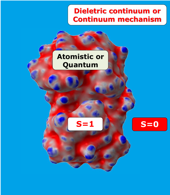
Figure 1: An illustration of differential geometric based solvation models. The minimum curvature is mapped on the Laplace-Beltrami surface of protein penicillopepsin (PDB ID 2web).

Our DG theory of the solvent-solute interface can be extend into a full solvation model by incorporating a variational formulation of the PB theory [129, 130] as well as a model of nonpolar solute-solvent interactions [1] following a similar approach by Dzubiella, Swanson, and McCammon [131]. We have implemented our DG-based solvation models in the Eulerian formulation, where the solute boundary is embedded in the three-dimensional (3D) Euclidean space so evaluation of the electrostatic potential can be carried out directly [71]. We have also implemented our DG-based solvation models in the Lagrangian formulation [72] (see Fig. 1) wherein the solvent-solute interface is extracted as a sharp surface and subsequently used in solving the PB equation for the electrostatic potential. To account for solute response to solvent polarization, we recently introduced a quantum mechanical (QM) treatment of solute charges to our DG-based solvation models using density functional theory (DFT) [132]. Most recently, Wei and coworkers have taken a different treatment of non-electrostatic interactions between the solvent and solute in the DG based solvation models so that the resulting total energy functional and PB equations are consistent with more detailed descriptions of solvent densities at equilibrium [75, 76]. This multiscale approach self-consistently computes the solute charge density distribution which simultaneously minimizes both the DFT energy as well as the solvation energy contributions. The resulting model significantly extends the applicability of our solvation model to a broad class of molecules without the need for force-field parametrized charge terms. The resulting differential geometry implicit solvent model has been tested extensively and shows excellent performance when compared with experimental and explicit solvent reference datasets [71, 72, 132, 1, 133, 134, 75, 135, 136].

As mentioned above, a parallel line of research has been carried out by Dzubiella, Hansen, McCammon, and Li. Early work by Dzubiella and Hansen demonstrated the importance of the self-consistent treatment of polar and nonpolar interactions in solvation models [137, 138]. These observations were then incorporated into a self-consistent variational framework for polar and non-polar solvation behavior by Dzubiella, Swanson, and McCammon [131, 139] which shared many common elements with our earlier geometric flow approach but included an additional term to represent nonpolar energetic contributions from surface curvature. Li and co-workers then developed several mathematical methods for this variational framework based on level-set methods and related approaches [140, 141, 142] which they demonstrated and tested on a variety of systems [143, 144, 145]. Unlike our Eulerian representation [71], level-set methods typically give rise to models with sharp solvent-solute interfaces.

An immediate consequence of our models is that the surfaces generated are free of troublesome geometric singularities that commonly occur in conventional solvent-accessible and solvent-excluded surfaces [146, 147] and impact computational stability of methods (see Fig. 2 for a smooth surface profile). Addition, without using ad hoc molecular surfaces, both our solvation models and the models of Dzubiella et al. significantly reduce the number of free parameters that users must “fit” or adjust in applications to real-world systems [136]. Our recent work shows that physical parameters; i.e., pressure and surface tension, obtained from experimental data can be directly employed in our DG-based solvation models to achieve an accurate prediction of solvation energy [135].

In this chapter, we review a number of DG-based models. Initially, we discuss solvation models, i.e, nonpolar and polar solvation models at equilibrium. To improve the accuracy and make our models robust, quantum mechanics is applied to the solute’s electron structure. As an important extension, we also consider DG-based models for the dynamical processes at non-equilibrium settings, including applied external electrical field gradients and inhomogeneous solvent concentration across membrane proteins.

II.A Nonpolar solvation model

As discussed above, solvation free energy is typically divided into two contributions: polar and nonpolar components. In one popular description, polar portion refers to electrostatic contributions while the nonpolar component includes all other effects. Scaled particle theory (SPT) is often used to describe the hard-sphere interactions between the solute and the solvent by including the surface free energy and mechanical work of creating a cavity of the solute size in the solvent [148, 149].

The SPT model can be used in combination with other solute-solvent nonpolar interactions; e.g. [150, 131, 74, 71]:

$$G^{\rm{NP}}=\gamma A+pV+\int_{\Omega_{s}}Ud{\bf{r}},\quad{\bf r}\in{\mathbb{R}}^{3},$$ (1)

where the first two terms are from SPT and the last term is the free energy due to solvent-solute interactions. Here, $A$ and $V$ are the surface area and volume of the solute, respectively; $\gamma$ is the surface tension; $p$ is the hydrodynamic pressure; $U$ denotes the solvent-solute non-electrostatic interactions; and $\Omega_{s}$ is the solvent domain.

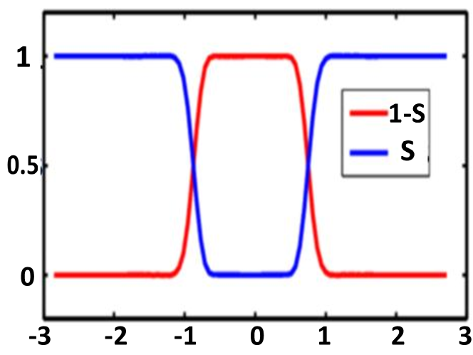
Figure 2: An illustration of the one-dimensional projection of the profiles of $S$ and $1-S$ functions along the $x$-axis.

In our earlier work, we have shown that the surface area in Eq. 1 can be evaluated via a two-dimensional (2D) integral for arbitrarily shaped molecules [123, 124]. For variation purposes, the total free functional must be set up as a 3D integral in ${\mathbb{R}}^{3}$. To this end, we take advantage of geometric measure theory by considering the mean surface area [74] and the coarea formula [151]:

$$A=\int_{0}^{1}\int_{S^{-1}(c)\bigcap\Omega}d\sigma dc=\int_{\Omega}|\nabla S({\bf{r}})|d{\bf{r}},\quad{\bf r}\in{\mathbb{R}}^{3},$$ (2)

where $\Omega$ denotes the whole computational domain and $0\leq S\leq 1$ is a hypersurface or simple surface function that characterizes the solute domain and embeds the 2D surface in ${\mathbb{R}}^{3}$; $1-S$ characterizes the solvent domain [71]. Using the function $S$, the volume in Eq. 1 can be defined as:

$$V=\int_{\Omega_{m}}d{\bf{r}}=\int_{\Omega}S({\bf{r}})d{\bf{r}},$$ (3)

where $\Omega_{m}$ is the solute domain. Note that $\Omega_{s}\cap\Omega_{m}$ is not empty because the surface function $S$ is a smooth function, which leads to overlap between $\Omega_{s}$ and $\Omega_{m}$ domains. The last term in Eq. 1 can be written in terms of $S$ as:

$$\int_{\Omega_{s}}Ud{\bf{r}}=\int_{\Omega}(1-S({\bf{r}}))Ud{\bf{r}}.$$ (4)

Therefore, we have the following nonpolar solvation free energy functional [74, 71, 1]:

$$G^{\rm NP} [S]=\int\left\{\gamma|\nabla S|+pS+(1-S)U\right\}d{\bf{r}}$$ (5)

which is in an appropriate form for variational analysis.

It is important to understand the nature of the solvent-solute non-electrostatic interaction, $U$. Assume that the aqueous environment has multiple species labeled by $\alpha$, and their interactions with each solute atom near the interface can be given by:

$$U = \sum_{\alpha}\rho_{\alpha}U_{\alpha}$$ (6)

$$= \sum_{\alpha}\rho_{\alpha}({\bf r})\sum_{j}U_{\alpha j}({\bf r})$$ (7)

where $\rho_{\alpha}({\bf r})$ is the density of $\alpha$th solution component, which may be charged or uncharged, and $U_{\alpha j}$ is an interaction potential between the $j$th atom of the solute and the $\alpha$th component of the solvent. For water that is free of other species, $\rho_{\alpha}({\bf r})$ is the water molecule density. In our earlier work [71, 72], we represented solvent-solute interactions using the Lennard-Jones potential. The full Lennard-Jones potential is singular and can cause computational difficulties [71]; however, Zhao has proposed a way to improve the integration stability in a realistic setting for proteins [127]. However, further mathematical algorithms are needed for this class of problems. The Weeks-Chandler-Anderson (WCA) decomposition of the potential, which separates the attractive and repulsive components [152], was also found to provide a good account of the attractive dispersion interaction in our earlier work [71, 72].

The interaction potential $U$ can be further modified to consider additional interactions, such as steric effects [153] and alternate descriptions of van der Waals interactions.

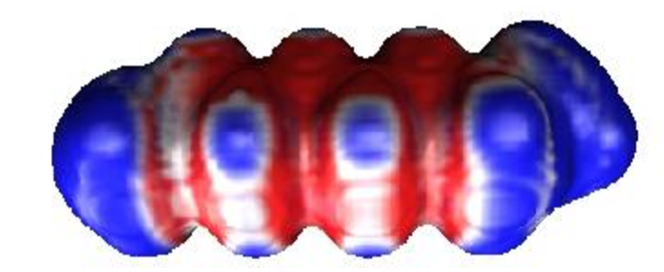
Figure 3: The final isosurfaces of a nonpolar compound projected with the corresponding van der Waals (vdW) potential for glycerol triacetate [1].

Table 1: Solvation energies calculated with the differential geometry nonpolar solvation model for a set of 11 alkanes in comparison with an explicit solvent model [154]. Errors are computed with respect to experimental data [155].

	Rep. part (kcal/mol)		Att. part (kcal/mol)		Total (kcal/mol)		Error (kcal/mol)
Compound	DG-NP	Explicit	DG-NP	Explicit	DG-NP	Explicit	DG-NP	Explicit
methane	4.71	5.72	-2.73	-3.31	1.98	2.41	-0.02	0.41
ethane	6.65	8.07	-4.75	-5.44	1.90	2.63	0.07	0.80
butane	10.30	10.10	-8.18	-7.21	2.12	2.89	0.04	0.81
propane	8.50	12.19	-6.45	-8.98	2.04	3.21	0.08	1.25
pentane	12.19	14.22	-9.82	-10.77	2.37	3.45	0.04	1.12
hexane	14.03	16.17	-11.54	-12.38	2.50	3.78	0.01	1.30
isobutane	10.14	11.91	-7.97	-8.88	2.16	3.03	-0.36	0.51
2-methylbutane	11.73	13.64	-9.35	-10.13	2.38	3.51	0.00	1.13
neopentane	11.81	13.62	-9.20	-10.39	2.61	3.23	0.11	0.73
cyclopentane	10.60	12.79	-9.43	-9.99	1.17	2.80	-0.03	1.60
cyclohexane	12.05	14.00	-10.78	-11.66	1.27	2.34	0.04	1.11

The Euler-Lagrange equation is used in our variational approach. By variation of the energy functional with respect to $S$, we arrive at an elliptic equation

$$\nabla\cdot\left(\gamma\frac{\nabla S}{|\nabla S|}\right)-p+U=0,$$ (8)

where $\nabla\cdot\left(\gamma\frac{\nabla S}{|\nabla S|}\right)$ is a mean curvature term as the surface tension $\gamma$ is treated as a constant. A standard computational procedure used in our earlier work [121, 123, 124] involves converting Eq. 8 into a parabolic equation by introducing an artificial time variable:

$$\frac{\partial S}{\partial t} = |\nabla S|\left[\nabla\cdot\left(\gamma\frac{\nabla S}{|\nabla S|}\right)+V_{\rm NP}\right]$$ (9)

where $V_{\rm NP}=-p+U$ is a potential-driving term for the time-dependent problem. Equation 9 is a generalized Laplace-Beltrami equation whose solution leads to the minimization of the nonpolar solvation free energy with respect to the surface function $S$.

The accuracy of the nonpolar solvation model performance is crucial to the success of other expanded versions of the differential geometry formalism. In particular, as the electrostatic effect and its associated approximation error are excluded, the major factor impacting the nonpolar solvation model is the solvent-solute boundary, which is governed by the DG-based formalism. Therefore, the nonpolar model provides the most direct and essential validation of the DG-based models. In our recent work [1], the DG-based nonpolar solvation (DG-NP) model was tested using a large number of nonpolar compounds. Table 1 presents a small portion of our results [1] compared with an explicit nonpolar model [154] and experimental data [155]. The solvation free energy is decomposed into repulsive and attractive parts, showing dramatic cancellations. The predicted total nonpolar solvation energies are in good agreement with experimental measurements. More extensive validation of our DG-NP model can be found in an earlier paper [1].

II.B Incorporating polar solvation with a Poisson-Boltzmann model

Most biomolecules are either charged or highly polarized; therefore, electrostatic interactions are indispensable in their theoretical description. The energy of electrostatic interactions can be modeled by a number of theoretical approaches, including Poisson-Boltzmann (PB) theory [26, 27, 4, 3], polarizable continuum theory [20, 156], and the generalized Born approximation [8, 9]. In our work, we incorporate PB theory for the polar solvation free energy and optimize the electrostatic solvation energy in our variational procedure.

Using the surface function $S$ and electrostatic potential $\Phi$, a PB model for the polar solvation free energy can be expressed by [74, 71]:

$$G_{\rm{polar}}=\int\left\{S\left[-\frac{\epsilon_{m}}{2}|\nabla\Phi|^{2}+\Phi\ \varrho\right]+(1-S)\left[-\frac{\epsilon_{s}}{2}|\nabla\Phi|^{2}-k_{B}T\sum_{\alpha}\rho_{\alpha 0}\left(e^{-\frac{q_{\alpha}\Phi+U_{\alpha}-\mu_{\alpha 0}}{k_{B}T}}-1\right)\right]\right\}d{\bf{r}},$$ (10)

where $\epsilon_{s}$ and $\epsilon_{m}$ are the dielectric constants of the solvent and solute, respectively, and $\varrho$ represents the fixed charge density of the solute. The charge density is often modeled by a point charge approximation $\varrho=\sum_{j}Q_{j}\delta({\bf{r}}-{\bf{r}}_{j})$, with $Q_{j}$ denoting the partial charge of the $j$th atom in the solute. $k_{B}$ is the Boltzmann constant; $T$ is the temperature; $\rho_{\alpha 0}$ denotes the reference bulk concentration of the $\alpha$th solvent species; and $q_{\alpha}$ denotes the charge valence of the $\alpha$th solvent species, which is zero for an uncharged solvent component. In Eq. 10, the form of the Boltzmann distribution [75] is different from that featured in our earlier work [74, 71].

$$\rho_{\alpha}=\rho_{\alpha 0}e^{-\frac{q_{\alpha}\Phi+U_{\alpha}-\mu_{\alpha 0}}{k_{B}T}}$$ (11)

with $\mu_{\alpha 0}$ being a relative reference chemical potential that reflects differences in the equilibrium activities of the different chemical species, and thus their concentrations. The extra term $e^{-\frac{U_{\alpha}}{k_{B}T}}$ in Eq. 11 describes the solvent-solute interactions near the interface beyond those implicitly represented by $S$. Therefore, $e^{-\frac{U_{\alpha}}{k_{B}T}}$ provides a non-electrostatic correction to the charge density near the interface.

The resulting total free energy functional for the full solvation system was first proposed in 2012 [75]:

$$\begin{aligned} G^{\rm PB}_{\rm{total}}[S,\Phi]&=\int\left\{\gamma|\nabla S|+pS+S\left[-\frac{\epsilon_{m}}{2}|\nabla\Phi|^{2}+\Phi\ \varrho\right]\right.\\ &\left.+(1-S)\left[-\frac{\epsilon_{s}}{2}|\nabla\Phi|^{2}-k_{B}T\sum_{\alpha}\rho_{\alpha 0}\left(e^{-\frac{q_{\alpha}\Phi+U_{\alpha}-\mu_{\alpha 0}}{k_{B}T}}-1\right)\right]\right\}d{\bf{r}}.\end{aligned}$$ (12)

Note that the energy functional (Eq. 12) differs from that in our earlier work [74, 71] and that of Dzubiella et al. [131, 139] not only in terms of the Boltzmann distribution, but also in the solvent-solute interactions $(1-S)U$, which is omitted in the present form. As shown in Section III, the present form is consistent with the DG-based Poisson-Nernst-Planck (PNP) theory at equilibrium. The DG-based PNP model offers a more detailed description of solvent densities based on fundamental laws of physics. As a result, the formalism of the DG-based full solvation model should agree with that of the DG-based PNP model at equilibrium.

The total solvation free energy in Eq. 12 is expressed as a functional of the surface function $S$ and electrostatic potential $\Phi$. Therefore, the total solvation free energy functional can be minimized with respect to $S$ and $\Phi$ via the variational principle. Variation with respect to $S$ leads to:

$$\begin{aligned} -\nabla\cdot\left(\gamma\frac{\nabla S}{|\nabla S|}\right)+p-\frac{\epsilon_{m}}{2}|\nabla\Phi|^{2}+\Phi\ \varrho+\frac{\epsilon_{s}}{2}|\nabla\Phi|^{2}+k_{B}T\sum_{\alpha}\rho_{\alpha 0}\left(e^{-\frac{q_{\alpha}\Phi+U_{\alpha}-\mu_{\alpha 0}}{k_{B}T}}-1\right)=0.\end{aligned}$$ (13)

Using the same procedure discussed earlier, we construct the following generalized Laplace-Beltrami equation:

$$\frac{\partial S}{\partial t} = |\nabla S|\left[\nabla\cdot\left(\gamma\frac{\nabla S}{|\nabla S|}\right)+V_{\rm PB}\right],$$ (14)

where the potential driven term is given by

$$V_{\rm PB}=-p+\frac{\epsilon_{m}}{2}|\nabla\Phi|^{2}-\Phi\ \varrho-\frac{\epsilon_{s}}{2}|\nabla\Phi|^{2}-k_{B}T\sum_{\alpha}\rho_{\alpha 0}\left(e^{-\frac{q_{\alpha}\Phi+U_{\alpha}-\mu_{\alpha 0}}{k_{B}T}}-1\right).$$ (15)

As in the nonpolar case, solving the generalized Laplace-Beltrami equation (14) generates the solvent-solute interface through the function $S$. Variation with respect to $\Phi$ gives the generalized PB (GPB) equation:

$$-\nabla\cdot\left(\epsilon(S)\nabla\Phi\right)=S\varrho+(1-S)\sum_{\alpha}q_{\alpha}\rho_{\alpha 0}e^{-\frac{q_{\alpha}\Phi+U_{\alpha}-\mu_{\alpha 0}}{k_{B}T}},$$ (16)

where $\epsilon(S)=(1-S)\epsilon_{s}+S\epsilon_{m}$ is the generalized permittivity function. As shown in our earlier work [74, 71], $\epsilon(S)$ is a smooth dielectric function gradually varying from $\epsilon_{m}$ to $\epsilon_{s}$. Thus, the solution procedure of the GPB equation avoids many numerical difficulties of solving elliptic equations with discontinuous coefficients [157, 158, 159, 160, 161] in the standard PB equation.

Equations 14 and 16 are solved for the surface function $S$ and electrostatic potential $\Phi$, respectively. These coupled “Laplace-Beltrami and Poisson-Boltzmann” equations are the governing equation for the DG-based solvation model in the Eulerian representation. The Lagrangian representation of the DG-based solvation model has also been derived [72]. Both the Eulerian and Lagrangian solvation models have been shown [71, 72] to be essentially equivalent and provide very good predictions of solvation energies for a diverse range of compounds.

II.C Improving Poisson-Boltzmann model charge distributions with quantum mechanics

While our earlier DG-based solvation models resolved the problem of ad hoc solute-solvent boundaries, they depended on existing force field parameters for atomic partial charge and radius assignments. Most force field models are parametrized for a certain class of molecules or materials which often limits their transferability and applicability. In particular, fixed partial charges do not account for charge rearrangement during the solvation process [162, 163, 164]. Therefore, a quantum solvation model that can self-consistently update the charge density of the solute molecule during solvation offers the promise of improving the accuracy and transferability of our DG-based solvation model.

A quantum mechanical formulation of solute charge density can be pursued in a number of ways. The most accurate treatment is the one that uses quantum mechanical first principle or ab initio approaches. However, the ab initio calculation of the electronic structure of a macromolecule is currently prohibitively expensive due to the large number of degrees of freedom. A variety of elegant theories and algorithms have been developed in the literature to reduce the dimensionality of this many-body problem [165, 166, 167, 168, 169, 170, 171, 172]. In earlier work from the Wei group, a density functional theory (DFT) treatment of solute electron distributions was incorporated into our DG-based solvation model [132]. In this work, we review the basic formulation and present an improved DG-DFT model for solvation analysis. Our goal is to construct a DG-DFT based solvation model that will significantly improve the accuracy of existing solvation models and still be orders of magnitude faster than explicit solvent models.

DFT uses functionals of single-electron distributions to represent multi-electron properties so that the total dimensionality is dramatically reduced. To combine DFT with our DG-based solvation formulation, we define the kinetic energy functional as:

$$G_{\rm kin}[n]=\sum_{j}\int S({\bf r})\frac{\hbar^{2}}{2m}|\nabla\psi_{j}({\bf r})|^{2}d{\bf r}$$ (17)

where $n$ is the total electron density, $m({\bf r})$ is the position-dependent electron mass, $\hbar=\frac{h}{2\pi}$ with $h$ being the Planck constant, and $\psi_{j}({\bf r})$ are the Kohn-Sham orbitals. The total electron density $n$ is obtained by:

$$n({\bf r})=\sum_{i}|\psi_{i}|^{2},$$ (18)

where the summation is over all of the Kohn-Sham orbitals.

In the absence of external potentials, the electrostatic potential energy of nuclei and electrons can be represented by the Coulombic interactions among the electrons and nuclei. There are three groups of electrostatic interactions: interactions between nuclei, interactions between electrons and nuclei, and interactions between electrons. Following the Born-Oppenheimer approximation, we neglect nuclei interactions in our DG-based model. Using Coulomb’s law, the repulsive interaction between electrons can be expressed as the Hartree term:

$$U_{ee}[n]=\frac{1}{2}\int\frac{e_{C}^{2}n({\bf r})n({\bf r}^{\prime})}{\epsilon({\bf r})|{\bf r}-{\bf r}^{\prime}|}d{\bf r}^{\prime},$$ (19)

where $e_{C}$ is the unit charge of an electron; $\epsilon({\bf r})$ is the position-dependent electric permittivity; and ${\bf r}$ and ${\bf r}^{\prime}$ are positions of two interacting electrons. Equation 19 $U_{ee}[n]$ involves nonlinear functions of the electron density $n$ which implies the need for iterative numerical variational methods, even in the absence of solvent density. The attractive interactions between electrons and nuclei are given by:

$$U_{en}[n]=-\sum_{I}\frac{e_{C}^{2}n({\bf r})Z_{I}}{\epsilon({\bf r})|{\bf r}-{\bf R}_{I}|}$$ (20)

where $Z_{I}$ is the charge of the nucleus. The total potential energy functional is then given by

$$G_{\rm potential}=\int_{\Omega}S({\bf r})\left(U_{ee}[n]+U_{ne}[n]+E_{\rm XC}[n]\right)d{\bf r},$$ (21)

where the last term, $E_{\rm XC}$, is the exchange-correlation potential, which approximates the many-particle interactions in the solute molecule.

Intuitively, it appears that the total free energy functional for the DG-based model is the simple summation of the polar, nonpolar, kinetic, and potential energy. However, such a summation will lead to double counting because of the coupling among different energy terms. For example, the electrostatic energy depends on the charge density, which, in turn, depends on the kinetic and potential energies of electrons. Additionally, the electrostatic potential serves as a variable in the polar energy functional and also serves as a known input in the potential energy of electrons through solution of the Poisson equation in vacuum $(\epsilon=1)$

$$-\nabla^{2}\phi_{v}({\bf r})=\rho^{v}_{\rm total}({\bf r}),$$ (22)

where $\phi_{v}$ is the electrostatic potential in vacuum and $\rho^{v}_{\rm total}=n_{v}+n_{n}$ with $n_{v}({\bf r})$ being the electron density in vacuum and $n_{n}$ the density of nuclei. The solution of the Poisson equation in vacuum is:

$$\phi_{v}({\bf r})=\int\frac{e_{C}n_{v}({\bf r}^{\prime})}{|{\bf r}-{\bf r}^{\prime}|}d{\bf r^{\prime}}-\sum_{I}\frac{e_{C}Z_{I}}{|{\bf r}-{\bf R}_{I}|}.$$ (23)

Of note, the solution to Eq. 23 is the exact total Coulombic potential of the electron-electron and electron-nucleus interactions. Therefore, we do not need to include $U_{ee}[n]$ and $U_{en}[n]$ terms in the total free energy functional.

Based on the preceding discussions, we propose a total free energy functional for solutes at equilibrium:

$$G_{\rm total}^{\rm DFT-PB}[S,\phi,n]=\int_{\Omega}\left\{\gamma|\nabla S({\bf r})|+pS({\bf r})+S({\bf r})\left[\rho_{\rm total}\phi-\frac{1}{2}\epsilon_{m}|\nabla\phi|^{2}\right]\right.\\ \left.+(1-S({\bf r}))\left[-\frac{\epsilon_{s}}{2}|\nabla\Phi|^{2}-k_{B}T\sum_{\alpha}\rho_{\alpha 0}\left(e^{-\frac{q_{\alpha}\Phi+U_{\alpha}-\mu_{\alpha 0}}{k_{B}T}}-1\right)\right]\right.\\ +\left.S({\bf r})\left[\sum_{j}\frac{\hbar^{2}}{2m}|\nabla\psi_{j}|^{2}+E_{\rm XC}[n]\right]\right\}d{\bf r},$$ (24)

where the first row is the nonpolar energy functional; the second row is the electrostatic energy functional; and the last row is the electronic energy functional, which is confined to the solute region by $S({\bf r})$. As already discussed, the term $\rho_{\rm total}=n_{v}+n_{n}$ also contributes to the Coulombic potentials of the electron-electron and electron-nucleus interactions. This total free energy functional provides a starting point for the derivation of governing equations for the DG-based solvation models, as well as the basis for evaluation of solvation free energies.

The governing equations for the DG-based solvation model with quantum mechanical charge distributions are determined by the calculus of variations. As before, variation of Eq. 24 with respect to the electrostatic potential $\phi$ gives the generalized Poisson-Boltzmann (GPB) equation [74, 71]:

$$-\nabla\cdot(\epsilon(S)\nabla\phi)=S\rho_{\rm total}+(1-S)\sum_{\alpha=1}^{N_{c}}\rho_{\alpha 0}q_{\alpha}e^{-\frac{q_{\alpha}\Phi+U_{\alpha}-\mu_{\alpha 0}}{k_{B}T}},$$ (25)

where the dielectric function is defined as before: $\epsilon(S)=(1-S)\epsilon_{s}+S\epsilon_{m}$. In a solvent without salt, the GPB equation is simplified to be the Poisson equation:

$$-\nabla\cdot(\epsilon(S)\nabla\phi)=S\rho_{\rm total}.$$ (26)

This equation and Eq. 25 are similar to the model described in the previous section (Sec. II.B). However, in the present multiscale model, the charge source $\rho_{\rm total}$ is determined by solving the Kohn-Sham equations rather than by the fixed charges $\rho_{m}=\sum_{j}Q_{j}\delta({\bf r}-{\bf r}_{j})$.

Variation of Eq. 24 with respect to the surface function $S$ gives a Laplace-Beltrami equation [123, 124, 74, 71]:

$$\frac{\partial S}{\partial t}=|\nabla S|\left[\nabla\cdot\left(\gamma\frac{\nabla S}{|\nabla S|}\right)+V_{\rm DFT-PB}\right],$$ (27)

where

$$V_{\rm DFT-PB}=-p+\frac{1}{2}\epsilon_{m}|\nabla\phi|^{2}-\frac{1}{2}\epsilon_{s}|\nabla\Phi|^{2}-k_{B}T\sum_{\alpha=1}^{N_{c}}\rho_{\alpha 0}\left(e^{-\frac{q_{\alpha}\Phi+U_{\alpha}-\mu_{\alpha 0}}{k_{B}T}}-1\right)\\ -\rho_{\rm total}\Phi-\sum_{j}\frac{\hbar^{2}}{2m}|\nabla\psi_{j}|^{2}-E_{\rm XC}[n]$$ (28)

The electronic potentials in the last row of this equation have relatively small contributions to $V_{\rm DFT-PB}$ at equilibrium due to the fact that they essentially are confined inside the solute molecular domain. Note that Eq. 27 has the same structure as the potential-driven geometric flow equation defined in the models presented in earlier in this chapter. As $t\rightarrow\infty$, the initial profile of $S$ evolves into a steady-state solution, which offers an optimal surface function $S$.

Finally, to derive the equation for the electronic wavefunction, we minimize the energy functional with respect to the wavefunction $\psi_{j}^{*}({\bf r})$, subject to the Lagrange multiplier ($\sum_{i}E_{i}\left(\delta_{ij}-\int S\psi_{i}({\bf r})\psi_{j}^{*}({\bf r})d{\bf r}\right)$) for the orthogonality of wavefunctions to arrive at the Kohn-Sham equation

$$\left(-\frac{\hbar^{2}}{2m}\nabla^{2}+U_{\rm eff}\right)\psi_{j}=E_{j}\psi_{j},\quad{\rm with}\quad U_{\rm eff}({\bf r})=q\Phi+V_{\rm XC}[n],$$ (29)

where the Lagrange multiplier constants $E_{i}$ can be interpreted as energy expectation values, $V_{\rm XC}[n]=\frac{dE_{\rm XC}[n]}{dn}$, and $q\phi$ is the potential contribution from Coulombic interactions. These electrostatic interactions can be calculated by the GPB equation (27) with a given total charge density. Eq. 29 does not directly depend on the solvent characteristic function $S$, so existing DFT packages can be used in our computations with minor modifications.

To integrate our continuum model with standard DFT algorithms, Wei and co-workers introduce the reaction field potential $\Phi_{\rm RF}=\Phi-\Phi_{0}$ with $\Phi_{0}$ being the solution of the Poisson equation in homogeneous media [132]. The reaction field potential is the electric potential induced by the polarized solvent and its incorporation leads to the following effective energy function

$$U_{\rm eff}({\bf r})=q\Phi+V_{\rm XC}[n]=q\Phi_{\rm RF}+U^{0}_{\rm eff}({\bf r})$$ (30)

where $U^{0}_{\rm eff}({\bf r})=q\Phi_{0}+V_{\rm XC}[n]$ is the traditional Kohn-Sham potential available in most DFT algorithms. The reaction field potential also appears in the Hamiltonian of the solute in the quantum calculation [173, 174, 175] and can be obtained from the electrostatic computation in the framework of the continuum models developed above. In summary, the inclusion of quantum mechanical charge distributions in the DG-based continuum model involves two components: 1) the classical electrostatic problem of determining the solvent reaction field potential with the quantum mechanically calculated charge density and 2) the quantum mechanical problem of calculating the electron charge density with fixed nucleus charges in the presence of the reaction field potential. To carry out these computations, an intuitive, self-consistent, iterative procedure can be constructed to solve the quantum equations for the electron distribution and the continuum electrostatic equations for the reaction field potential [173, 176, 20, 174, 175].

After solving the Kohn-Sham equation, the QM-based charge density can be incorporated into the solvation model in two different ways. Our preferred approach is to apply the continuous QM charge density directly to the PB equation as a source term. However, it is also possible to fit the QM charge density into atomic point charges or multipoles for use as the source term [177, 178, 179]. This second approach is most useful when the DG-DFT scheme is used in conjunction with other molecular simulation approaches, such as MM-PBSA or docking.

III Differential geometry-based electrolyte transport models

It is well-known that implicit solvent models use both discrete and continuum representations of molecular systems to reduce the number of degrees of freedom; this philosophy and methodology of implicit solvent models can be extended to more general multiscale formulations. A variety of DG-based multiscale models have been introduced in an earlier paper of Wei [74]. Theory for the differential geometry of surfaces provides a natural means to separate the microscopic solute domain from the macroscopic solvent domain so that appropriate physical laws are applied to applicable domains. This portion of the chapter focuses specifically on the extension of the equilibrium electrostatics models described above to non-equilibrium transport problems which are relevant to a variety of chemical and biological systems, such as molecular motors, ion channels, fuel cells and nanofluidics, with chemically or biologically relevant behavior that occurs far from equilibrium [74, 75, 76].

Another class of DG-based multiscale models involves the dynamics and transport of ion channels, transmembrane transporters and nanofluidics. In new multiscale models developed by the Wei group, the total energy functionals are modified with additional chemical energies to account for spatially inhomogeneous ion density distribution and charge fluxes due to applied external field gradients and inhomogeneous solvent concentrations across membranes. The Nernst-Planck equation is constructed using Fick’s law via a generalized chemical potential governed by the variational principle. Together with the Laplace-Beltrami equation for the surface function and Poisson equation for electrostatic potential, the resulting DG-based PNP theory reduces to our PB theory at equilibrium [75]. The PNP equation has been thoroughly studied in the biophysical literature [180, 181, 182, 183, 184, 185, 186, 187]; however, a DG-based formulation of the PNP offers many of the advantages that DG-based solvation models described above provide: elimination of several ad hoc parameters from the model and a framework in which to incorporate more complicated solution phenomena such as strong correlations between ions and confinement-induced ion steric effects. Additionally, compared with conventional PNP models [180, 181, 182, 183, 184, 185, 186, 187], the DG-based PNP models include nonpolar solvation free energy and thus can be used to predict the full solvation energy against experimental data, in addition to the usual current-voltage curves [75].

III.A A differential geometry-based Poisson-Nernst-Planck model

The GPB and Laplace-Beltrami models discussed in the previous section were obtained from a variational principle applied to equilibrium systems. For chemical and biological systems far from equilibrium, it is necessary to incorporate additional equations (e.g., the Nernst-Planck equation) to describe the dynamics of charged particles. Various DG-based Nernst-Planck equations have derived from mass conservation laws in earlier work by Wei and co-workers [74, 75]. We outline the basic derivation here. For simplicity in derivation, we assume that the flow stream velocity vanishes ($|{\bf v}|=0$) and we omit the chemical reactions in our present discussion.

The chemical potential contribution to the free energy consists a homogeneous reference term and the entropy of mixing [188]:

$$G_{\rm{chem}}=\int\sum_{\alpha}\left\{\left(\mu^{0}_{\alpha}-\mu_{\alpha 0}\right)\rho_{\alpha}+k_{B}T\rho_{\alpha}{\rm{ln}}\ \frac{\rho_{\alpha}}{\rho_{\alpha 0}}-k_{B}T\left(\rho_{\alpha}-\rho_{\alpha 0}\right)\right\}d{\bf{r}},$$ (31)

where $\mu^{0}_{\alpha}$ is the reference chemical potential of the $\alpha$th species at which the associated ion concentration is $\rho_{0\alpha}$ in a homogeneous system (e.g., $\Phi=U_{\alpha}=\mu_{\alpha 0}=0$). Here, $k_{B}T\rho_{\alpha}{\rm{ln}}\ \frac{\rho_{\alpha}}{\rho_{\alpha 0}}$ is the entropy of mixing, and $-k_{B}T\left(\rho_{\alpha}-\rho_{\alpha 0}\right)$ is a relative osmotic term [189]. The chemical potential of species $\alpha$ can be obtained by variation with respect to $\rho_{\alpha}$:

$$\frac{\delta G_{\rm{chem}}}{\delta\rho_{\alpha}}\Rightarrow\mu^{\rm chem}_{\alpha}=\mu^{0}_{\alpha}-\mu_{\alpha 0}+k_{B}T{\rm{ln}}\ \frac{\rho_{\alpha}}{\rho_{\alpha 0}}.$$ (32)

Note that at equilibrium, $\mu^{\rm chem}_{\alpha}\neq 0$ and $\rho_{\alpha}\neq\rho_{\alpha 0}$ because of possible external electrical potentials, charged solutes, solvent-solute interactions, and charged species interactions. This chemical potential energy term can be combined with the polar and and nonpolar contributions discussed in the previous sections to give a total system free energy of

$$G^{\rm PNP}_{\rm{total}}[S,\Phi,\{\rho_{\alpha}\}]=\int\left\{\gamma|\nabla S|+pS+(1-S)U\right.\\ \left.+S\left[-\frac{\epsilon_{m}}{2}|\nabla\Phi|^{2}+\Phi\ \varrho\right]+(1-S)\left[-\frac{\epsilon_{s}}{2}|\nabla\Phi|^{2}+\Phi\sum_{\alpha}\rho_{\alpha}q_{\alpha}\right]\right.\\ \left.+(1-S)\sum_{\alpha}\left[\left(\mu^{0}_{\alpha}-\mu_{\alpha 0}\right)\rho_{\alpha}+k_{B}T\rho_{\alpha}{\rm{ln}}\ \frac{\rho_{\alpha}}{\rho_{\alpha 0}}-k_{B}T\left(\rho_{\alpha}-\rho_{\alpha 0}\right)+\lambda_{\alpha}\rho_{\alpha}\right]\right\}d{\bf{r}},$$ (33)

where $\lambda_{\alpha}$ is a Lagrange multiplier, which is required to ensure appropriate physical properties at equilibrium [188]. In this functional, the first row is the nonpolar solvation free energy contribution, the second row is the polar solvation free energy contribution, and the third row is chemical potential energy contribution. A unique aspect of this PNP formulation is the inclusion of nonpolar solvation free energy contribution to the functional (see Eq. 1).

While electrostatic interactions provide a strong driving force for many biomolecular phenomena, they are not the only source of ion-ion and ion-solute interactions. In the heterogeneous environment where biomolecules interact with a range of aqueous ions, counterions, and other solvent molecules, electrostatic interactions often manifest themselves in a variety of different forms related to polarization, hyperpolarization, vibrational and rotational averages, screening effects, etc. For example, size effects have been shown to play an important role in macromolecular interactions [190, 134, 191, 192, 193, 194]. Another important effect is the change of ion-water interactions due to geometric confinement, which is commonly believed to result in channel selectivity for sodium and/or potassium ions [134]. In past papers by Wei and co-workers, these types of interactions are called “non-electrostatic interactions” or “generalized correlations” [134, 75] and are incorporated into the DG-based models by modifying Eqs. 6 and 7:

$$U = \sum_{\alpha}\rho_{\alpha}U_{\alpha}$$

$$U_{\alpha} = \sum_{j}U_{\alpha j}({\bf r})+\sum_{\beta}U_{\alpha\beta}({\bf r}),$$ (34)

where the subscript $\beta$ runs over all solvent components, including ions and water. In general, we denote $U_{\alpha}$ as any possible non-electrostatic interactions in the system. The inclusion of these non-electrostatic interactions does not change the derivation or the form of other expressions presented in the preceding section. The total free energy functional (Eq. 33) is a function of the surface function $S$, electrostatic potential $\Phi$, and the ion concentration $\rho_{\alpha}$. The governing equations for the system are derived using the variational principle.

We first derive the generalized Poisson equation by the variation of the total free energy functional with respect to the electrostatic potential $\Phi$. The resulting generalized Poisson equation is:

$$-\nabla\cdot\left(\epsilon(S)\nabla\Phi\right)=S\varrho+(1-S)\sum_{\alpha}\rho_{\alpha}q_{\alpha},$$ (35)

where $\epsilon(S)=(1-S)\epsilon_{s}+S\epsilon_{m}$ is an interface-dependent dielectric profile. The generalized Poisson equation (Eq. 35) involves the surface function $S$ and the densities of ions $\rho_{\alpha}$, which are to be determined. Variation with respect to the ion density $\rho_{\alpha}$ leads to the relative generalized potential $\mu^{\rm gen}_{\alpha}$

$$\frac{\delta G^{\rm PNP}_{\rm{total}}}{\delta\rho_{\alpha}}\Rightarrow\mu^{\rm gen}_{\alpha}=\mu^{0}_{\alpha}-\mu_{\alpha 0}+k_{B}T{\rm{ln}}\ \frac{\rho_{\alpha}}{\rho_{\alpha 0}}+q_{\alpha}\Phi+U_{\alpha}+\lambda_{\alpha}=\mu^{\rm chem}_{\alpha}+q_{\alpha}\Phi+U_{\alpha}+\lambda_{\alpha}.$$ (36)

We require $\mu^{\rm gen}_{\alpha}$, rather than $\mu^{\rm chem}_{\alpha}$, to vanish at equilibrium. Therefore, we require:

$$\lambda_{\alpha} = -\mu^{0}_{\alpha}$$

$$\rho_{\alpha} = \rho_{\alpha 0}e^{-\frac{q_{\alpha}\Phi+U_{\alpha}-\mu_{\alpha 0}}{k_{B}T}}.$$ (37)

Using these relations, the relative generalized chemical potential $\mu^{\rm gen}_{\alpha}$ can be rewritten as:

$$\mu^{\rm gen}_{\alpha}=k_{B}T{\rm{ln}}\ \frac{\rho_{\alpha}}{\rho_{\alpha 0}}\ +q_{\alpha}\Phi+U_{\alpha}-\mu_{\alpha 0}.$$ (38)

Wei and co-workers derived a similar quantity from a slightly different perspective in an earlier paper [195]. Note that this chemical potential consists of contributions from the entropy of mixing, electrostatic potential, solvent-solute interaction, and the position-independent reference chemical potential. For many biomolecular transport problems, diffusion is the major mechanism for transport and relaxation to equilibrium. By Fick’s first law, the diffusive ion flux is ${\bf J}_{\alpha}=-D_{\alpha}\rho_{\alpha}\nabla\frac{\mu^{\rm gen}_{\alpha}}{k_{B}T}$ with $D_{\alpha}$ being the diffusion coefficient of species $\alpha$. The diffusion equation for the mass conservation of species $\alpha$ at the absence of steam velocity is $\frac{\partial\rho_{\alpha}}{\partial t}=-\nabla\cdot{\bf J}_{\alpha}$, which results in the generalized Nernst-Planck equation:

$$\frac{\partial\rho_{\alpha}}{\partial t}=\nabla\cdot\left[D_{\alpha}\left(\nabla\rho_{\alpha}+\frac{\rho_{\alpha}}{k_{B}T}\nabla(q_{\alpha}\Phi+U_{\alpha})\right)\right],$$ (39)

where $q_{\alpha}\Phi+U_{\alpha}$ is a form of the mean field potential. In the absence of solvent-solute interactions, Eq. 39 reduces to the standard Nernst-Planck equation.

Using the Euler-Lagrange equation, one can derive an elliptic equation for the surface function $S$ and, introducing an artificial time as discussed earlier in this chapter, this can be transformed into a parabolic equation:

$$\frac{\partial S}{\partial t} = |\nabla S|\left[\nabla\cdot\left(\gamma\frac{\nabla S}{|\nabla S|}\right)+V_{\rm PNP}\right],$$ (40)

where the driving term is

$$V_{\rm PNP} = -p+U+\frac{\epsilon_{m}}{2}|\nabla\Phi|^{2}-\Phi\ \varrho-\frac{\epsilon_{s}}{2}|\nabla\Phi|^{2}+\Phi\sum_{\alpha}\rho_{\alpha}q_{\alpha}$$

$$+\sum_{\alpha}\left[k_{B}T\left(\rho_{\alpha}{\rm{ln}}\ \frac{\rho_{\alpha}}{\rho_{\alpha 0}}-\rho_{\alpha}+\rho_{\alpha 0}\right)-\mu_{\alpha 0}\rho_{\alpha}\right].$$

Equations 39, 35, and 40 form a coupled system of equations describing the surface function $S$, charge concentrations $\rho_{\alpha}$, and electrostatic potential $\Phi$. This coupled system differs from the original PNP equations through the coupling of the surface definition are to charge concentrations and electrostatics. We call this DG-based system the “Laplace-Beltrami Poisson-Nernst-Planck” (LB-PNP) model.

In general, the total free energy functional of the DG-based PNP model in Eq. 33 differs from that of the DG-based PB model in Eq. 12. The difference also exists between the surface-driven term $V_{\rm PNP}$ in the charge transport model and $V_{\rm BP}$ in the solvation model. Moreover, $\rho_{\alpha}$ in the charge transport model is determined by the Nernst-Planck equation (39) rather than the Boltzmann factor. However, if the charge flux is zero for the electrodiffusion system, the PNP model is known to be equivalent to the PB model [196]. Note that at equilibrium, the relative generalized potential vanishes everywhere, and the result is the equilibrium constraint given in Eq. 37. Therefore, by using the equilibrium constraint, the total free energy functional in Eq. 33 becomes [75]:

$$G^{\rm PNP}_{\rm{total}}\longrightarrow G^{\rm PB}_{\rm{total}},\quad~{}{\rm as}~{}\rho_{\alpha}\longrightarrow\rho_{\alpha 0}e^{-\frac{q_{\alpha}\Phi+U_{\alpha}-\mu_{\alpha 0}}{k_{B}T}}.$$ (42)

This relationship shows that, under the equilibrium assumption, the total free energy functional for the charge transport model reduces to the equilibrium solvation model presented earlier (Eq. 12). Furthermore, for the surface-driven functions of the generalized LB equation, it is easy to show [75] that under the equilibrium constraint, one has:

$$V_{\rm PNP}\longrightarrow V_{\rm BP},\quad~{}{\rm as}~{}\rho_{\alpha}\longrightarrow\rho_{\alpha 0}e^{-\frac{q_{\alpha}\Phi+U_{\alpha}-\mu_{\alpha 0}}{k_{B}T}}.$$ (43)

This consistency between the DG-based PNP and PB models is a crucial aspect of this non-equilibrium theory of charge transport. Numerical simulations in Wei’s group have confirmed this consistency [75].

III.B Quantum mechanical charge distributions in the Poisson-Nernst-Planck model

As with the equilibrium solvation models introduced earlier, it is also possible to incorporate quantum mechanical effects into the non-equilibrium transport model. Our motivation is to account for non-equilibrium ion fluxes and induced response in the electronic structure of the solute or membrane protein. To this end, we combine our DG-based DFT model with our DG-based PNP model as illustrated in Fig. 4 to develop a free energy functional and derive the associated governing equations.

The free energy functional is a combination of four models (nonpolar, PB, PNP, and DFT) in a manner which avoids energetic double-counting. Four variables are used ($S,\Phi,\{\rho_{\alpha}\}$, and $n$) to minimize the total energy. The resulting free energy functional has the form:

$$G^{\rm DFT-PNP}_{\rm{total}}[S,\Phi,\{\rho_{\alpha}\},n]=\int\left\{\gamma|\nabla S|+pS+(1-S)U\right.\\ \left.+S\left[-\frac{\epsilon_{m}}{2}|\nabla\Phi|^{2}+\rho_{\rm total}\Phi\right]+(1-S)\left[-\frac{\epsilon_{s}}{2}|\nabla\Phi|^{2}+\Phi\sum_{\alpha}\rho_{\alpha}q_{\alpha}\right]\right.\\ \left.+(1-S)\sum_{\alpha}\left[\left(\mu^{0}_{\alpha}-\mu_{\alpha 0}\right)\rho_{\alpha}+k_{B}T\rho_{\alpha}{\rm{ln}}\ \frac{\rho_{\alpha}}{\rho_{\alpha 0}}-k_{B}T\left(\rho_{\alpha}-\rho_{\alpha 0}\right)+\lambda_{\alpha}\rho_{\alpha}\right]\right.\\ +\left.S\left[\sum_{j}\frac{\hbar^{2}}{2m}|\nabla\psi_{j}|^{2}+E_{\rm XC}[n]\right]\right\}d{\bf r},$$ (44)

where the first row is the nonpolar solvation energy functional, the second row is electrostatic energy density of solvation, the third row is the chemical energy functional of solvent ions, and the last row is the energy density of solute electrons in the DFT representation, as explained in earlier sections. Note that this coupled form places some restrictions on the potential $U$: in particular, care must be taken to avoid double-counting dispersive and repulsive interactions that are already accounted for in the quantum mechanical treatment. Using this function, the derivation of governing equations is straightforward. For the sake of completeness, we discuss all of the governing equations of this new model (as follows).

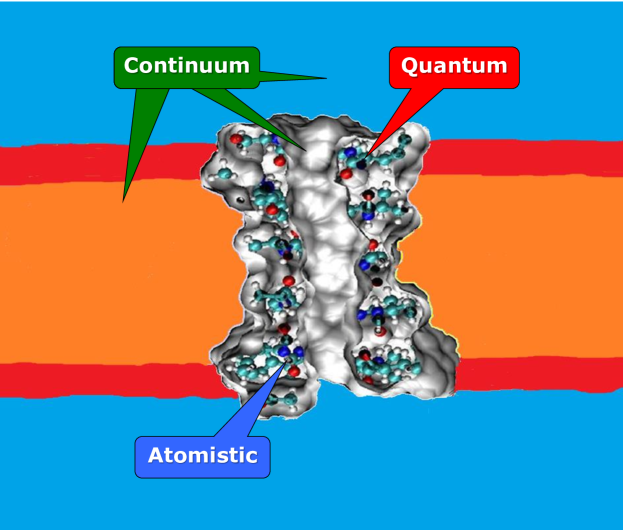
Figure 4: An illustration of the differential geometry-based DFT-PNP model for ion channels.

As before, variation of the total free energy functional with respect to the electrostatic potential $\Phi$ gives rise to the generalized Poisson equation:

$$-\nabla\cdot\left(\epsilon(S)\nabla\Phi\right)=S\rho_{\rm total}+(1-S)\sum_{\alpha}\rho_{\alpha}q_{\alpha},$$ (45)

where $\epsilon(S)=(1-S)\epsilon_{s}+S\epsilon_{m}$ is an interface-dependent dielectric profile. The charge sources in Eq. 45 are the total charge density $\rho_{\rm total}$ of the solute molecule and the ionic density $\sum_{\alpha}\rho_{\alpha}q_{\alpha}$ of aqueous species. The former is determined by DFT, while the latter is estimated by the Nernst-Planck theory. At equilibrium (37), the generalized Poisson equation (45) reduces to the GPB equation given in Eq. 25.

The procedure for deriving the Nernst-Planck equation is the same as discussed in the previous section. We first carry out the variation with respect to $\rho_{\alpha}$ to obtain the relative generalized potential. Next, Fick’s laws of diffusion are employed to construct the generalized Nernst-Planck equation:

$$\frac{\partial\rho_{\alpha}}{\partial t}=\nabla\cdot\left[D_{\alpha}\left(\nabla\rho_{\alpha}+\frac{\rho_{\alpha}}{k_{B}T}\nabla(q_{\alpha}\Phi+U_{\alpha})\right)\right].$$ (46)

Formally, this equation has the same form as the generalized Nernst-Planck equation in the last section. However, to evaluate $U_{\alpha}$, possible effects stemming from the quantum mechanical representation of the electronic structure must be considered.

As discussed previously, variation with respect to the surface function $S$ leads to a generalized Laplace-Beltrami equation after the introduction of an artificial time:

$$\frac{\partial S}{\partial t} = |\nabla S|\left[\nabla\cdot\left(\gamma\frac{\nabla S}{|\nabla S|}\right)+V_{\rm DFT-PNP}\right],$$ (47)

where the potential driving term is given by

$$V_{\rm DFT-PNP}=-p+U+\frac{\epsilon_{m}}{2}|\nabla\Phi|^{2}-\Phi\ \varrho-\frac{\epsilon_{s}}{2}|\nabla\Phi|^{2}+\Phi\sum_{\alpha}\rho_{\alpha}q_{\alpha}\\ +\sum_{\alpha}\left[k_{B}T\left(\rho_{\alpha}{\rm{ln}}\ \frac{\rho_{\alpha}}{\rho_{\alpha 0}}-\rho_{\alpha}+\rho_{\alpha 0}\right)-\mu_{\alpha 0}\rho_{\alpha}\right]-\sum_{j}\frac{\hbar^{2}}{2m}|\nabla\psi_{j}|^{2}-E_{\rm XC}[n].$$ (48)

At equilibrium (Eq. 37) $V_{\rm DFT-PNP}$ becomes $V_{\rm DFT-PB}$. Eq. 47 is coupled to all other quantities, $\Phi,\rho_{\alpha}$ and $n$. Fast solutions to this type of equation remains an active research issue [124, 71, 197].

In the present multiscale DFT formalism, the governing Kohn-Sham equation is obtained via the minimization of the energy functional with respect to $\psi_{j}^{*}({\bf r})$, subject to the Lagrange multiplier ($\sum_{i}E_{i}\left(\delta_{ij}-\int S\psi_{i}({\bf r})\psi_{j}^{*}({\bf r})d{\bf r}\right)$),

$$\left(-\frac{\hbar^{2}}{2m}\nabla^{2}+q\Phi+V_{\rm XC}[n]\right)\psi_{j}=E_{j}\psi_{j}.$$ (49)

Although the Kohn-Sham equation does not explicitly involve the surface function and ion densities, the electrostatic potential energy $q\Phi$ is calculated by the GPB equation (45) which is coupled with solvent charge density and surface function. As such, electronic response to ion fluxes in the ion channel is included in the present model.

Equations 45, 46, 47, and 49 form a complete set of governing equations which are strongly coupled to each other. Therefore, these equations can be solved by nonlinear iterative procedures [198, 133, 134] and efficient second-order algorithms [71, 72, 132, 1].

IV Concluding remarks

Geometric analysis, which combines differential geometry (DG) with partial differential equations (PDEs), has generated great successes in the physical sciences and engineering. In the past decade, DG-based solvation models have been introduced for biomolecular modeling. This new methodology has been tested over hundreds of molecular test cases, ranging from nonpolar molecules to large proteins. Our DG-based solvation models use the differential geometry of surfaces theory as a natural means to separate microscopic domains for biomolecules from macroscopic domains for solvents and to couple continuum descriptions with discrete atomistic or quantum representations. The goal of our DG-based formalism is to achieve an accurate prediction of essential physical observables while efficiently reducing the dimensionality of complex biomolecular systems. An important technique used in our approach is the construction of total free energy functionals for various biomolecular systems, which enables us to put various scales into an equal footing. Variational principles are applied to the total energy functional to derive coupled governing PDEs for biomolecular systems.

This chapter has focused on equilibrium and non-equilibrium models of electrolyte solutions around biomolecules. However, the Wei group has also extended this formalism to the multiscale modeling of other systems and biological processes. One class of multiscale models developed in the Wei group is a DG-based quantum treatment of proton transport [133, 134]. Proton transport underpins the molecular mechanisms in a variety of systems, including transmembrane ATPases as well as other proton pumps and translocators [199]. The significant quantum effects in proton permeation require quantum mechanical models, while the large number of degrees of freedom demands a multiscale treatment [200, 201]. In the multiscale approach developed by the Wei group, a new DFT is formulated based on Boltzmann statistics, rather than Fermi-Dirac statistics, for protons in the solvent while treating water molecules as a dielectric continuum. The membrane protein is described in atomistic detail and densities of other ions in the solvent are approximated via Boltzmann distributions, following an approach introduced in our earlier Poisson-Boltzmann-Nernst-Planck theory [195]. The resulting multiscale proton model provides excellent predictions of experimental current-voltage relationships [133, 134]. Another class of DG-based multiscale models has been proposed by Wei et al. for alternative MM and/or continuum elasticity (CE) description of solute molecules, as well as continuum fluid mechanics formulation of the solvent [74, 75, 76, 202]. The idea is to endow the DG-based multiscale paradigm with the ability to handle excessively large macromolecules by elasticity description, manage conformational changes with MM, and deal with macromolecular-flow interaction via fluid mechanics. The theory of continuum elasticity with atomic rigidity (CEWAR) also has been introduced [202] and treats the molecular shear modulus as a continuous function of atomic rigidity. Thus, the dynamic complexity of integrating time-dependent governing equations for a macromolecular system is separated from the static complexity of determining the flexibility at given time step. In CEWAR, the more time-consuming dynamics is approximated using continuum elasticity theory while the less-time-consuming static analysis is pursued with atomic description. A recent multidomain formulation by Wei and co-workers allows each different part of a macromolecule to have a different physical description [76]. Efficient geometric modeling strategies associated with DG-based multiscale models have been developed in both Lagrangian-Eulerian [203, 204] and Eulerian representations [205]. Algorithms for curvature evaluation and volumetric and surface meshing have been developed for organelles, subcellular structures, and multiprotein complexes [203] and have been combined with electrostatic analysis for the prediction of protein-ligand binding sites [205].

Literature cited

Literature cited

- [1] Z. Chen, Shan Zhao, J. Chun, D. G. Thomas, N. A. Baker, P. B. Bates, and G. W. Wei. Variational approach for nonpolar solvation analysis. Journal of Chemical Physics, 137(084101), 2012.
- [2] N. A. Baker. Biomolecular applications of Poisson-Boltzmann methods. In K. B. Lipkowitz, R. Larter, and T. R. Cundari, editors, Reviews in Computational Chemistry, volume 21. John Wiley and Sons, Hoboken, NJ, 2005.
- [3] M. E. Davis and J. A. McCammon. Electrostatics in biomolecular structure and dynamics. Chemical Reviews, 94:509–21, 1990.
- [4] K. A. Sharp and B. Honig. Electrostatic interactions in macromolecules - theory and applications. Annual Review of Biophysics and Biophysical Chemistry, 19:301–332, 1990.
- [5] B. Honig and A. Nicholls. Classical electrostatics in biology and chemistry. Science, 268(5214):1144–9, 1995.
- [6] B. Roux and T. Simonson. Implicit solvent models. Biophysical Chemistry, 78(1-2):1–20, 1999.
- [7] R. Jinnouchi and A. B. Anderson. Electronic structure calculations of liquid-solid interfaces: Combination of density functional theory and modified Poisson-Boltzmann theory. PHYSICAL REVIEW B, 77(245417), 2008.
- [8] B. N. Dominy and C. L. Brooks, III. Development of a generalized Born model parameterization for proteins and nucleic acids. Journal of Physical Chemistry B, 103(18):3765–3773, 1999.
- [9] D. Bashford and D. A. Case. Generalized Born models of macromolecular solvation effects. Annual Review of Physical Chemistry, 51:129–152, 2000.
- [10] V. Tsui and D. A. Case. Molecular dynamics simulations of nucleic acids with a generalized Born solvation model. Journal of the American Chemical Society, 122(11):2489–2498, 2000.
- [11] A. Onufriev, D. A. Case, and D. Bashford. Effective Born radii in the generalized Born approximation: the importance of being perfect. Journal of Computational Chemistry, 23(14):1297–304, 2002.
- [12] E. Gallicchio, L. Y. Zhang, and R. M. Levy. The SGB/NP hydration free energy model based on the surface generalized Born solvent reaction field and novel nonpolar hydration free energy estimators. Journal of Computational Chemistry, 23(5):517–29, 2002.
- [13] J. Zhu, E. Alexov, and B. Honig. Comparative study of generalized Born models: Born radii and peptide folding. Journal of Physical Chemistry B, 109(7):3008–22, 2005.
- [14] P. Koehl. Electrostatics calculations: latest methodological advances. Current Opinion in Structural Biology, 16(2):142–51, 2006.
- [15] H. Tjong and H. X. Zhou. GBr6NL: A generalized Born method for accurately reproducing solvation energy of the nonlinear Poisson-Boltzmann equation. Journal of Chemical Physics, 126:195102, 2007.
- [16] J. Mongan, C. Simmerling, J. A. McCammon, D. A. Case, and A. Onufriev. Generalized Born model with a simple, robust molecular volume correction. Journal of Chemical Theory and Computation, 3(1):159–69, 2007.
- [17] D. Chen, G. W. Wei, X. Cong, and G. Wang. Computational methods for optical molecular imaging. Communications in Numerical Methods in Engineering, 25:1137–1161, 2009.
- [18] J. A. Grant, B. T. Pickup, M. T. Sykes, C. A. Kitchen, and A. Nicholls. The Gaussian Generalized Born model: application to small molecules. Physical Chemistry Chemical Physics, 9:4913–22, 2007.
- [19] Mahito Chiba, Dmitri G. Fedorov, and Kazuo Kitaura. Polarizable continuum model with the fragment molecular orbital-based time-dependent density functional theory. Journal of Computational Chemistry, 29:2667–2676, 2008.
- [20] Jacopo Tomasi, Benedetta Mennucci, and Roberto Cammi. Quantum mechanical continuum solvation models. Chem. Rev., 105:2999–3093, 2005.
- [21] R. Improta, V. Barone, G. Scalmani, and M. J. Frisch. A state-specific polarizable continuum model time dependent density functional theory method for excited state calculations in solution. Journal of Chemical Physics, 125(054103), 2006.
- [22] Y. Takano and K. N. Houk. Benchmarking the conductor-like polarizable continuum model (cpcm) for aqueous solvation free energies of neutral and ionic organic molecules. Journal of Chemical Theory and Computation, 1(1):70–77, 2005.
- [23] E. Cances, B. Mennucci, and J. Tomasi. A new integral equation formalism for the polarizable continuum model: Theoretical background and applications to isotropic and anisotropic dielectrics. Journal of Chemical Physics, 107:3032 – 3041, 1997.
- [24] V Barone, M. Cossi, and J. Tomasi. A new definition of cavities for the computation of solvation free energies by the polarizable continuum model. Journal of Chemical Physics, 107:3210–3221, 1997.
- [25] M. Cossi, V. Barone, R. Cammi, and J. Tomasi. Ab initio study of solvated molecules: A new implementation of the polarizable continuum model. Chemical Physics Letters, 255:327–335, 1996.
- [26] G. Lamm. The Poisson-Boltzmann equation. In K. B. Lipkowitz, R. Larter, and T. R. Cundari, editors, Reviews in Computational Chemistry, pages 147–366. John Wiley and Sons, Inc., Hoboken, N.J., 2003.
- [27] F. Fogolari, A. Brigo, and H. Molinari. The Poisson-Boltzmann equation for biomolecular electrostatics: a tool for structural biology. Journal of Molecular Recognition, 15(6):377–92, 2002.
- [28] Y. C. Zhou, M. Feig, and G. W. Wei. Highly accurate biomolecular electrostatics in continuum dielectric environments. Journal of Computational Chemistry, 29:87–97, 2008.
- [29] N. A. Baker. Improving implicit solvent simulations: a Poisson-centric view. Current Opinion in Structural Biology, 15(2):137–43, 2005.
- [30] D. Beglov and B. Roux. Solvation of complex molecules in a polar liquid: an integral equation theory. Journal of Chemical Physics, 104(21):8678–8689, 1996.
- [31] R. R. Netz and H. Orland. Beyond Poisson-Boltzmann: Fluctuation effects and correlation functions. European Physical Journal E, 1(2-3):203–14, 2000.
- [32] Christian Holm, Patrick Kekicheff, and Rudolf Podgornik. Electrostatic effects in soft matter and biophysics; NATO Science Series. Kluwer Academic Publishers, Boston, 2001.
- [33] L. David, R. Luo, and M. K. Gilson. Comparison of generalized Born and Poisson models: Energetics and dynamics of HIV protease. Journal of Computational Chemistry, 21(4):295–309, 2000.
- [34] A. Onufriev, D. Bashford, and D. A. Case. Modification of the generalized Born model suitable for macromolecules. Journal of Physical Chemistry B, 104(15):3712–3720, 2000.
- [35] Philip Weinzinger, Sup Hannongbua, and Pete Wolschann. Molecular mechanics PBSA ligand binding energy and interaction of efavirenz derivatives with HIV-1 reverse transcriptase. Journal of Enzyme Inhibition and Medicinal Chemistry, 20(2):129–134, 2005.
- [36] J. M. J. Swanson, R. H. Henchman, and J. A. McCammon. Revisiting free energy calculations: A theoretical connection to MM/PBSA and direct calculation of the association free energy. Biophysical Journal, 86(1):67–74, 2004.
- [37] Christopher S. Page and Paul A. Bates. Can MM-PBSA calculations predict the specificities of protein kinase inhibitors? Journal of Computational Chemistry, 27(16):1990–2007, 2006.
- [38] Jian J. Tan, Wei Z. Chen, and Cun X. Wang. Investigating interactions between HIV-1 gp41 and inhibitors by molecular dynamics simulation and MM-PBSA/GBSA calculations. Journal of Molecular Structure: Theochem., 766(2-3):77–82, 2006.
- [39] I. Massova and P. A. Kollman. Computational Alanine Scanning To Probe Protein-Protein Interactions: A Novel Approach To Evaluate Binding Free Energies. Journal of the American Chemical Society, 121(36):8133–43, 1999.
- [40] D. Bashford and M. Karplus. p’s of ionizable groups in proteins: atomic detail from a continuum electrostatic model. Biochemistry, 29(44):10219–25, 1990.
- [41] J. Antosiewicz, J. A. McCammon, and M. K. Gilson. The determinants of ps in proteins. Biochemistry, 35(24):7819–7833, 1996.
- [42] J. Li, C. L. Fisher, J. L. Chen, D. Bashford, and L. Noodleman. Calculation of redox potentials and pKa values of hydrated transition metal cations by a combined density functional and continuum dielectric theory. Inorganic Chemistry, 35(16):4694–702, 1996.
- [43] J. E. Nielsen and G. Vriend. Optimizing the hydrogen-bond network in Poisson-Boltzmann equation-based pK(a) calculations. Proteins, 43(4):403–412, 2001.
- [44] C. M. MacDermaid and G. A. Kaminski. Electrostatic polarization is crucial for reproducing pKa shifts of carboxylic residues in turkey ovomucoid third domain. Journal of Physical Chemistry B, 111(30):9036–44, 2007.
- [45] C. L. Tang, E. Alexov, A. M. Pyle, and B. Honig. Calculation of pKas in RNA: On the structural origins and functional roles of protonated nucleotides. Journal of Molecular Biology, 366(5):1475–96, 2007.
- [46] J. E. Nielsen, K. V. Andersen, B. Honig, R. W. W. Hooft, G. Klebe, G. Vriend, and R. C. Wade. Improving macromolecular electrostatics calculations. Protein Engineering, 12(8):657–662, 1999.
- [47] A. S. Yang, M. R. Gunner, R. Sampogna, K. Sharp, and B. Honig. On the calculation of pK(a)s in proteins. Proteins-Structure Function and Genetics, 15(3):252–265, 1993.
- [48] R. E. Georgescu, E. G. Alexov, and M. R. Gunner. Combining conformational flexibility and continuum electrostatics for calculating pKas in proteins. Biophysical Journal, 83(4):1731–1748, 2002.
- [49] William M. Matousek, Barbara Ciani, Carolyn A. Fitch, Bertrand E. Garcia-Moreno, Richard A. Kammerer, and Andrei T. Alexandrescu. Electrostatic contributions to the stability of the GCN4 leucine zipper structure. Journal of Molecular Biology, 374(1):206–19, 2007.
- [50] H. Li, A. D. Robertson, and J. H. Jensen. Very fast empirical prediction and rationalization of protein pka values. Proteins, 61(4):704–21, 2005.
- [51] H. Li, A. D. Robertson, and J. H. Jensen. The determinants of carboxyl pKa values in turkey ovomucoid third domain. Proteins, 55(3):689–704, 2004.
- [52] C. Tan, L. Yang, and R. Luo. How well does Poisson-Boltzmann implicit solvent agree with explicit solvent? A quantitative analysis. Journal of Physical Chemistry B, 110(37):18680–18687, 2006.
- [53] N. V. Prabhu, M. Panda, Q. Y. Yang, and K. A. Sharp. Explicit ion, implicit water solvation for molecular dynamics of nucleic acids and highly charged molecules. J. Comput. Chem., 29:1113–1130, 2008.
- [54] N. V. Prabhu, P. Zhu, and K. A. Sharp. Implementation and testing of stable, fast implicit solvation in molecular dynamics using the smooth-permittivity finite difference Poisson-Boltzmann method. Journal of Computational Chemistry, 25(16):2049–2064, 2004.
- [55] R. Luo, L. David, and M. K. Gilson. Accelerated Poisson-Boltzmann calculations for static and dynamic systems. Journal of Computational Chemistry, 23(13):1244–53, 2002.
- [56] Q. Lu and R. Luo. A Poisson-Boltzmann dynamics method with nonperiodic boundary condition. Journal of Chemical Physics, 119(21):11035–11047, 2003.
- [57] W. Geng and G. W. Wei. Multiscale molecular dynamics using the matched interface and boundary method. J Comput. Phys., 230(2):435–457, 2011.
- [58] J. D. Madura, J. M. Briggs, R. C. Wade, M. E. Davis, B. A. Luty, A. Ilin, J. Antosiewicz, M. K. Gilson, B. Bagheri, L. R. Scott, and J. A. McCammon. Electrostatics and diffusion of molecules in solution - simulations with the University of Houston Brownian Dynamics program. Computer Physics Communications, 91(1-3):57–95, 1995.
- [59] R. R. Gabdoulline and R. C. Wade. Brownian dynamics simulation of protein-protein diffusional encounter. Methods-a Companion to Methods in Enzymology, 14(3):329–341, 1998.
- [60] A. H. Elcock, R. R. Gabdoulline, R. C. Wade, and J. A. McCammon. Computer simulation of protein-protein association kinetics: Acetylcholinesterase-fasciculin. Journal of Molecular Biology, 291(1):149–162, 1999.
- [61] D. Sept, A. H. Elcock, and J. A. McCammon. Computer simulations of actin polymerization can explain the barbed-pointed end asymmetry. Journal of Molecular Biology, 294(5):1181–1189, 1999.
- [62] Y. Cheng, J. K. Suen, RadiÄ-Z., S. D. Bond, M. J. Holst, and J. A. McCammon. Continuum simulations of acetylcholine diffusion with reaction-determined boundaries in neuromuscular junction models. Biophysical Chemistry, 127(3):129–39, 2007.
- [63] Y. Cheng, J. K. Suen, D. Zhang, S. D. Bond, Y. Zhang, Y. Song, N. A. Baker, C. L. Bajaj, M. J. Holst, and J. A. McCammon. Finite element analysis of the time-dependent Smoluchowski equation for acetylcholinesterase reaction rate calculations. Biophysical Journal, 92(10):3397–406, 2007.
- [64] D. Zhang, J. Suen, Y. Zhang, Z. Radic, P. Taylor, M. Holst, C. Bajaj, N. A. Baker, and J. A. McCammon. Tetrameric mouse acetylcholinesterase: Continuum diffusion rate calculations by solving the steady-state Smoluchowski equation using finite element methods. Biophysical Journal, 88(3):1659–65, 2005.
- [65] Y. Song, Y. Zhang, C. L. Bajaj, and N. A. Baker. Continuum diffusion reaction rate calculations of wild-type and mutant mouse acetylcholinesterase: Adaptive finite element analysis. Biophysical Journal, 87(3):1558–66, 2004.
- [66] Y. Song, Y. Zhang, T. Shen, C. L. Bajaj, J. A. McCammon, and N. A. Baker. Finite element solution of the steady-state Smoluchowksi equation for rate constant calculations. Biophysical Journal, 86(4):2017–2029, 2004.
- [67] J. Warwicker and H. C. Watson. Calculation of the electric potential in the active site cleft due to alpha-helix dipoles. Journal of Molecular Biology, 157(4):671–9, 1982.
- [68] D. Petrey and B. Honig. GRASP2: Visualization, surface properties, and electrostatics of macromolecular structures and sequences. Methods in Enzymology, 374:492–509, 2003.
- [69] N. A. Baker and J. A. McCammon. Electrostatic interactions. In P. Bourne and H. Weissig, editors, Structural Bioinformatics, pages 427–440. John Wiley & Sons, Inc., New York, 2003.
- [70] N. A. Baker. Poisson-Boltzmann methods for biomolecular electrostatics. Methods in Enzymology, 383:94–118, 2004.
- [71] Z. Chen, N. A. Baker, and G. W. Wei. Differential geometry based solvation models I: Eulerian formulation. J. Comput. Phys., 229:8231–8258, 2010.
- [72] Z. Chen, N. A. Baker, and G. W. Wei. Differential geometry based solvation models II: Lagrangian formulation. J. Math. Biol., 63:1139– 1200, 2011.
- [73] P. Ren, J. Chun, D. G. Thomas, M. J. Schnieders, M. Marucho, J. Zhang, and N. A. Baker. Biomolecular electrostatics and solvation: a computational perspective. Quart. Rev. Biophys., 2013.
- [74] G. W. Wei. Differential geometry based multiscale models. Bulletin of Mathematical Biology, 72:1562 – 1622, 2010.
- [75] Guo-Wei Wei, Qiong Zheng, Zhan Chen, and Kelin Xia. Variational multiscale models for charge transport. SIAM Review, 54(4):699 – 754, 2012.
- [76] Guo-Wei Wei. Multiscale, multiphysics and multidomain models I: Basic theory. Journal of Theoretical and Computational Chemistry, 12(8):1341006, 2013.
- [77] J. Andrew Grant, Barry T. Pickup, and Anthony Nicholls. A smooth permittivity function for Poisson-Boltzmann solvation methods. Journal of Computational Chemistry, 22(6):608–640, 2001.
- [78] J. Grant and B. Pickup. A gaussian description of molecular shape. Journal of Physical Chemistry, 99:3503–3510, 1995.
- [79] B. Lee and F. M. Richards. The interpretation of protein structures: estimation of static accessibility. J Mol Biol, 55(3):379–400, 1971.
- [80] F. M. Richards. Areas, volumes, packing, and protein structure. Annual Review of Biophysics and Bioengineering, 6(1):151–176, 1977.
- [81] R. S. Spolar, J. H. Ha, and M. T. Record Jr. Hydrophobic effect in protein folding and other noncovalent processes involving proteins. Proceedings of the National Academy of Sciences of the United States of America, 86(21):8382–8385, 1989.
- [82] J. R. Livingstone, R. S. Spolar, and M. T. Record Jr. Contribution to the thermodynamics of protein folding from the reduction in water-accessible nonpolar surface area. Biochemistry, 30(17):4237–44, 1991.
- [83] Peter B. Crowley and Adel Golovin. Cation-pi interactions in protein-protein interfaces. Proteins: Structure, Function, and Bioinformatics, 59(2):231–239, 2005.
- [84] Leslie A. Kuhn, Michael A. Siani, Michael E. Pique, Cindy L. Fisher, Elizabeth D. Getzoff, and John A. Tainer. The interdependence of protein surface topography and bound water molecules revealed by surface accessibility and fractal density measures. Journal of Molecular Biology, 228(1):13–22, 1992.
- [85] C. A. S. Bergstrom, M. Strafford, L. Lazorova, A. Avdeef, K. Luthman, and P. Artursson. Absorption classification of oral drugs based on molecular surface properties. Journal of Medicinal Chemistry, 46(4):558–570, 2003.
- [86] Anatoly I. Dragan, Christopher M. Read, Elena N. Makeyeva, Ekaterina I. Milgotina, Mair E. Churchill, Colyn Crane-Robinson, and Peter L. Privalov. DNA binding and bending by HMG boxes: Energetic determinants of specificity. Journal of Molecular Biology, 343(2):371–393, 2004.
- [87] Richard M. Jackson and Michael J. Sternberg. A continuum model for protein-protein interactions: Application to the docking problem. Journal of Molecular Biology, 250(2):258–275, 1995.
- [88] V. J. Licata and N. M. Allewell. Functionally linked hydration changes in escherichia coli aspartate transcarbamylase and its catalytic subunit. Biochemistry, 36(33):10161–10167, 1997.
- [89] F. Dong, M. Vijaykumar, and H. X. Zhou. Comparison of calculation and experiment implicates significant electrostatic contributions to the binding stability of barnase and barstar. Biophysical Journal, 85(1):49–60, 2003.
- [90] F. Dong and H. X. Zhou. Electrostatic contribution to the binding stability of protein-protein complexes. Proteins, 65(1):87–102, 2006.
- [91] M. Nina, W. Im, and B. Roux. Optimized atomic radii for protein continuum electrostatics solvation forces. Biophysical Chemistry, 78(1-2):89–96, 1999.
- [92] J. M. J. Swanson, J. Mongan, and J. A. McCammon. Limitations of atom-centered dielectric functions in implicit solvent models. Journal of Physical Chemistry B, 109(31):14769–72, 2005.
- [93] X. Feng and A. Prohl. Analysis of a fully discrete finite element method for the phase field model and approximation of its sharp interface limits. Mathematics of Computation, 73:541–567, 2004.
- [94] J. Gomes and O. D. Faugeras. Using the vector distance functions to evolve manifolds of arbitrary codimension. Lecture Notes in Computer Science, 2106:1–13, 2001.
- [95] Karol Mikula and Daniel Sevcovic. A direct method for solving an anisotropic mean curvature flow of plane curves with an external force. Mathematical Methods in the Applied Sciences, 27(13):1545–1565, 2004.
- [96] Stanley Osher and Ronald P. Fedkiw. Level set methods: An overview and some recent results. J. Comput. Phys., 169(2):463–502, 2001.
- [97] A. Sarti, R. Malladi, and J. A. Sethian. Subjective surfaces: A geometric model for boundary completion. International Journal of Computer Vision, 46(3):201–221, 2002.
- [98] Catalina Sbert and Andreas F. Solé. 3d curves reconstruction based on deformable models. Journal of Mathematical Imaging and Vision, 18(3):211–223, 2003.
- [99] J. A. Sethian. Evolution, implementation, and application of level set and fast marching methods for advancing fronts. J. Comput. Phys., 169(2):503–555, 2001.
- [100] N. Sochen, R. Kimmel, and R. Malladi. A general framework for low level vision. Image Processing, IEEE Transactions on, 7(3):310–318, 1998.
- [101] Y. Zhang, G. Xu, and C. Bajaj. Quality meshing of implicit solvation models of biomolecular structures. Computer Aided Geometric Design, 23(6):510–30, 2006.
- [102] T. J. Willmore. Riemannian Geometry. Oxford University Press, USA, 1997.
- [103] S. Osher and J.A. Sethian. Fronts propagating with curvature-dependent speed: algorithms based on Hamilton-Jacobi formulations. Journal of computational physics, 79(1):12–49, 1988.
- [104] Leonid I. Rudin, Stanley Osher, and Emad Fatemi. Nonlinear total variation based noise removal algorithms. In Proceedings of the eleventh annual international conference of the Center for Nonlinear Studies on Experimental mathematics : computational issues in nonlinear science, pages 259–268, Amsterdam, The Netherlands, The Netherlands, 1992. Elsevier North-Holland, Inc.
- [105] Thomas Cecil. A numerical method for computing minimal surfaces in arbitrary dimension. J. Comput. Phys., 206(2):650–660, 2005.
- [106] David L. Chopp. Computing minimal surfaces via level set curvature flow. J. Comput. Phys., 106(1):77–91, 1993.
- [107] Peter Smereka. Semi-implicit level set methods for curvature and surface diffusion motion. Journal of Scientific Computing, 19(1):439–456, 2003.
- [108] David Mumford and Jayant Shah. Optimal approximations by piecewise smooth functions and associated variational problems. Communications on Pure and Applied Mathematics, 42(5):577–685, 1989.
- [109] P. Blomgren and T.F. Chan. Color TV: total variation methods for restoration of vector-valued images. Image Processing, IEEE Transactions on, 7(3):304–309, 1998.
- [110] V. Carstensen, R. Kimmel, and G. Sapiro. Geodesic active contours. International Journal of Computer Vision, 22:61–79, 1997.
- [111] Y. Li and F. Santosa. A computational algorithm for minimizing total variation in image restoration. IEEE Transactions on Image Processing, 5(6):987–95, 1996.
- [112] Stanley Osher and Leonid I. Rudin. Feature-oriented image enhancement using shock filters. SIAM Journal on Numerical Analysis, 27(4):919–940, 1990.
- [113] G. Sapiro and D. L. Ringach. Anisotropic diffusion of multivalued images with applications to color filtering. Image Processing, IEEE Transactions on, 5(11):1582–1586, 1996.
- [114] G. W. Wei. Generalized Perona-Malik equation for image restoration. IEEE Signal Processing Lett., 6:165–167, 1999.
- [115] G. W. Wei and Y. Q. Jia. Synchronization-based image edge detection. Europhysics Letters, 59(6):814–819, 2002.
- [116] Y. Wang, G. W. Wei, and Si-Yang Yang. Mode decomposition evolution equations. Journal of Scientific Computing, 50:495–518, 2012.
- [117] Y. Wang, G. W. Wei, and Si-Yang Yang. Partial differential equation transform – Variational formulation and Fourier analysis. International Journal for Numerical Methods in Biomedical Engineering, 27:1996–2020, 2011.
- [118] Y. Wang, G. W. Wei, and Si-Yang Yang. Selective extraction of entangled textures via adaptive pde transform. International Journal in Biomedical Imaging, 2012:Article ID 958142, 2012.
- [119] Q. Zheng, S. Y. Yang, and G. W. Wei. Molecular surface generation using PDE transform. International Journal for Numerical Methods in Biomedical Engineering, 28:291–316, 2012.
- [120] G. W. Wei, Y. H. Sun, Y. C. Zhou, and M. Feig. Molecular multiresolution surfaces. arXiv:math-ph/0511001v1, pages 1 – 11, 2005.
- [121] P. W. Bates, G. W. Wei, and S. Zhao. The minimal molecular surface. arXiv:q-bio/0610038v1, [q-bio.BM], 2006.
- [122] P. W. Bates, G. W. Wei, and S. Zhao. The minimal molecular surface. Midwest Quantitative Biology Conference, Mission Point Resort, Mackinac Island, MI:September 29 – October 1, 2006.
- [123] P. W. Bates, G. W. Wei, and Shan Zhao. Minimal molecular surfaces and their applications. Journal of Computational Chemistry, 29(3):380–91, 2008.
- [124] P. W. Bates, Z. Chen, Y. H. Sun, G. W. Wei, and S. Zhao. Geometric and potential driving formation and evolution of biomolecular surfaces. J. Math. Biol., 59:193–231, 2009.
- [125] L. T. Cheng, Joachim Dzubiella, Andrew J. McCammon, and B. Li. Application of the level-set method to the implicit solvation of nonpolar molecules. Journal of Chemical Physics, 127(8), 2007.
- [126] Z. Y. Yu and C. Bajaj. Computational approaches for automatic structural analysis of large biomolecular complexes. IEEE/ACM Trans Comput Biol Bioinform, 5:568–582, 2008.
- [127] Shan Zhao. Pseudo-time-coupled nonlinear models for biomolecular surface representation and solvation analysis. International Journal for Numerical Methods in Biomedical Engineering, 27:1964–1981, 2011.
- [128] Shan Zhao. Operator splitting adi schemes for pseudo-time coupled nonlinear solvation simulations. Journal of Computational Physics, 257:1000 – 1021, 2014.
- [129] K. A. Sharp and B. Honig. Calculating total electrostatic energies with the nonlinear Poisson-Boltzmann equation. Journal of Physical Chemistry, 94:7684–7692, 1990.
- [130] M. K. Gilson, M. E. Davis, B. A. Luty, and J. A. McCammon. Computation of electrostatic forces on solvated molecules using the Poisson-Boltzmann equation. Journal of Physical Chemistry, 97(14):3591–3600, 1993.
- [131] J. Dzubiella, J. M. J. Swanson, and J. A. McCammon. Coupling hydrophobicity, dispersion, and electrostatics in continuum solvent models. Physical Review Letters, 96:087802, 2006.
- [132] Z. Chen and G. W. Wei. Differential geometry based solvation models III: Quantum formulation. J. Chem. Phys., 135(194108), 2011.
- [133] Duan Chen, Zhan Chen, and G. W. Wei. Quantum dynamics in continuum for proton transport II: Variational solvent-solute interface. International Journal for Numerical Methods in Biomedical Engineering, 28:25 – 51, 2012.
- [134] Duan Chen and G. W. Wei. Quantum dynamics in continuum for proton transport—Generalized correlation. J Chem. Phys., 136:134109, 2012.
- [135] M. Daily, J. Chun, A. Heredia-Langner, G. W. Wei, and N. A. Baker. Origin of parameter degeneracy and molecular shape relationships in geometric-flow calculations of solvation free energies. Journal of Chemical Physics,, 139:204108, 2013.
- [136] D.G. Thomas, J. Chun, Z. Chen, G. W. Wei, and N. A. Baker. Parameterization of a geometric flow implicit solvation model. J. Comput. Chem., 24:687–695, 2013.
- [137] J. Dzubiella and J. P. Hansen. Reduction of the hydrophobic attraction between charged solutes in water. The Journal of Chemical Physics, 119(23):12049–12052, 2003.
- [138] J. Dzubiella and J.-P. Hansen. Competition of hydrophobic and coulombic interactions between nanosized solutes. The Journal of Chemical Physics, 121(11):5514–5530, September 2004.
- [139] J. Dzubiella, J. M. J. Swanson, and J. A. McCammon. Coupling nonpolar and polar solvation free energies in implicit solvent models. Journal of Chemical Physics, 124:084905, 2006.
- [140] J. Che, J. Dzubiella, B. Li, and J. A. McCammon. Electrostatic free energy and its variations in implicit solvent models. Journal of Physical Chemistry B, 112(10):3058–69, 2008.
- [141] Li-Tien Cheng, Yang Xie, Joachim Dzubiella, J. Andrew McCammon, Jianwei Che, and Bo Li. Coupling the level-set method with molecular mechanics for variational implicit solvation of nonpolar molecules. J. Chem. Theory Comput., 5:257–266, 2009.
- [142] Bo Li and Yanxiang Zhao. Variational implicit solvation with solute molecular mechanics: From Diffuse-Interface to Sharp-Interface models. SIAM journal on applied mathematics, 73(1):1–23, 2013.
- [143] P. Setny, Z. Wang, L. T. Cheng, B. Li, J. A. McCammon, and J. Dzubiella. Dewetting-Controlled binding of ligands to hydrophobic pockets. Physical Review Letters, 103(18):187801+, October 2009.
- [144] Li-Tien Cheng, Zhongming Wang, Piotr Setny, Joachim Dzubiella, Bo Li, and J. Andrew McCammon. Interfaces and hydrophobic interactions in receptor-ligand systems: A level-set variational implicit solvent approach. The Journal of Chemical Physics, 131(14):144102+, October 2009.
- [145] Shenggao Zhou, Kathleen E. Rogers, César A. de Oliveira, Riccardo Baron, Li-Tien Cheng, Joachim Dzubiella, Bo Li, and J. Andrew McCammon. Variational Implicit-Solvent modeling of Host–Guest binding: A case study on cucurbit[7]uril—. J. Chem. Theory Comput., 9(9):4195–4204, August 2013.
- [146] M. L. Connolly. Depth buffer algorithms for molecular modeling. J. Mol. Graphics, 3:19–24, 1985.
- [147] M. F. Sanner, A. J. Olson, and J. C. Spehner. Reduced surface: An efficient way to compute molecular surfaces. Biopolymers, 38:305–320, 1996.
- [148] F. H. Stillinger. Structure in aqueous solutions of nonpolar solutes from the standpoint of scaled-particle theory. J. Solution Chem., 2:141 – 158, 1973.
- [149] R. A. Pierotti. A scaled particle theory of aqueous and nonaqeous solutions. Chemical Reviews, 76(6):717–726, 1976.
- [150] J. A. Wagoner and N. A. Baker. Assessing implicit models for nonpolar mean solvation forces: the importance of dispersion and volume terms. Proceedings of the National Academy of Sciences of the United States of America, 103(22):8331–6, 2006.
- [151] H. Federer. Curvature Measures. Trans. Amer. Math. Soc., 93:418–491, 1959.
- [152] J. D. Weeks, D. Chandler, and H. C. Andersen. Role of repulsive forces in determining the equilibrium structure of simple liquids. Journal of Chemical Physics, 54(12):5237–47, 1971.
- [153] I. Borukhov and D. Andelman. Steric effects in electrolytes: A modified poisson-boltzmann equation. Phys. Rev. Lett., 79(3):435–438, 1997.
- [154] E. Gallicchio, M. M. Kubo, and R. M. Levy. Enthalpy-entropy and cavity decomposition of alkane hydration free energies: Numerical results and implications for theories of hydrophobic solvation. Journal of Physical Chemistry B, 104(26):6271–85, 2000.
- [155] S. Cabani, P. Gianni, V Mollica, and L Lepori. Group Contributions to the Thermodynamic Properties of Non-Ionic Organic Solutes in Dilute Aqueous Solution. Journal of Solution Chemistry, 10(8):563–595, 1981.
- [156] Y. Mei, C. G. Ji, and J. Z. H. Zhang. A new quantum method for electrostatic solvation energy of protein. J. Chem. Phys., 125(094906), 2006.
- [157] Shan Zhao and G. W. Wei. High-order FDTD methods via derivative matching for Maxwell’s equations with material interfaces. J. Comput. Phys., 200(1):60–103, 2004.
- [158] Y. C. Zhou, Shan Zhao, Michael Feig, and G. W. Wei. High order matched interface and boundary method for elliptic equations with discontinuous coefficients and singular sources. J. Comput. Phys., 213(1):1–30, 2006.
- [159] Y. C. Zhou and G. W. Wei. On the fictitious-domain and interpolation formulations of the matched interface and boundary (MIB) method. J. Comput. Phys., 219(1):228–246, 2006.
- [160] S. N. Yu, Y. C. Zhou, and G. W. Wei. Matched interface and boundary (MIB) method for elliptic problems with sharp-edged interfaces. J. Comput. Phys., 224(2):729–756, 2007.
- [161] S. N. Yu and G. W. Wei. Three-dimensional matched interface and boundary (MIB) method for treating geometric singularities. J. Comput. Phys., 227:602–632, 2007.
- [162] J. W. Ponder, C. J. Wu, P. Y. Ren, V. S. Pande, J. D. Chodera, M. J. Schnieders, I. Haque, D. L. Mobley, D. S. Lambrecht, R. A. DiStasio, M. Head-Gordon, G. N. I. Clark, M. E. Johnson, and T. Head-Gordon. Current status of the amoeba polarizable force field. J. Phys. Chem. B, 114:2549 – 2564, 2010.
- [163] A. Grossfield, P. Y. Ren, and J. W. Ponder. Ion solvation thermodynamics from simulation with a polarizable force field. J. Amer. Chem. Soc., 125:15671–15682, 2003.
- [164] M. J. Schnieders, N. A. Baker, P. Ren, and J. W. Ponder. Polarizable atomic multipole solutes in a Poisson-Boltzmann continuum. Journal of Chemical Physics, 126:124114, 2007.
- [165] Tai S. Lee, Darrin M. York, and Weitao Yang. Linear-scaling semiempirical quantum calculations for macromolecules. The Journal of Chemical Physics, 105(7):2744–2750, 1996.
- [166] W. T. Yang. Gradient correction in thomas-fermi theory. Physical Review A, 34(6):4575–4585, Dec 1986.
- [167] W. T. Yang. Direct calculation of electron density in density-functional theory. Physical Review Letters, 66:1438 – 1441, 1991.
- [168] W. T. Yang. A local projection method for the linear combination of atomic orbital implementation of density-functional theory. Journal of Chemical Physics, 94(2):1208–1214, Jan 1991.
- [169] W. T. Yang. Direct calculation of electron-density in density-functional theory. Physical Review Letters, 66(11):1438–1441, Mar 1991.
- [170] W. T. Yang. Abinitio approach for many-electron systems without invoking orbitals - an integral formulation of density-functional theory. Physical Review Letters, 59(14):1569–1572, Oct 1987.
- [171] S. Goedecker. Linear scaling electronic structure methods. Rev. Mod. Phys., 71:1085– 1123, 1999.
- [172] W. T. Yang. Abinitio approach for many-electron systems without invoking orbitals - an integral formulation of density-functional theory. Physical Review A, 38(11):5494–5503, Dec 1988.
- [173] D. J. Tannor, B. Marten, R. Murphy, R. A. Friesner, D. Sitkoff, A. Nicholls, M. Ringnalda, W. A. Goddard, and B. Honig. Accurate first principles calcualtion of molecular charge distribution and solvation energies from ab initio quantum mechanics and continuum dielectric theory. J. Am. Chem. Soc., 116:11875 – 11882, 1994.
- [174] M. L. Wang and C. F. Wong. Calculation of solvation free energy from quantum mechanical charge density and continuum dielectric theory. J. Phys. Chem. A, 110:4873–4879, 2006.
- [175] J.L. Chen, L. Noodleman, D.A. Case, and D. Bashford. Incorporating solvation effects into density functional electronic structure calculations. J. Phys. Chem., 98:11059– 11068, 1994.
- [176] V. Gogonea and K. M. Merz. Fully quantum mechanical description of proteins in solution. combining linear scaling quantum mechanical methodologies with the poisson-boltzmann equation. J. Phys. Chem. A, 103:5171–5188, 1999.
- [177] Weihua Geng, Sining Yu, and G. W. Wei. Treatment of charge singularities in implicit solvent models. Journal of Chemical Physics, 127:114106, 2007.
- [178] E. Sigfridsson and U. Ryde. Comparison of methods for deriving atomic charges from the electrostatic potential and moments. J. Comput. Chem., 19(4):377–395, 1998.
- [179] H Hu, Z. Y. Lu, and W. T. Yang. Fitting molecular electrostatic potentials from quantum mechanical calculations. Journal of Chemical Theory and Computation, 3:1004 – 1013, 2007.
- [180] W. Im and B. Roux. Ion permeation and selectivity of ompf porin:a theoretical study based on molecular dynamics, Brownian dynamics, and continuum electrodiffusion theory. J. Mol. Biol., 322:851–869, 2002.
- [181] D. Gillespie, W. Nonner, and R.S. Eisenberg. Density functional theory of charged, hard-sphere fluids. Phys. Rev. E, 68:031503, 2003.
- [182] B. S. Eisenberg and D Chen. Poisson-Nernst-Planck (PNP) theory of an open ionic channel. Biophysical Journal, 64:A22, 1993.
- [183] M. G. Kurnikova, R. D. Coalson, P. Graf, and A. Nitzan. A lattice relaxation algorithm for Three-Dimensional Poisson-Nernst-Planck theory with application to ion transport through the Gramicidin A channel. Biophysical Journal, 76:642–656, 1999.
- [184] Hirofumi Daiguji, Peidong Yang, and Arun Majumdar. Ion transport in nanofluidic channels. Nano Letters, 4(1):137–142, 2004.
- [185] J Cervera, B Schiedt, and P Ramirez. A poisson/nernst-planck model for ionic transport through synthetic conical nanopores. EPL (Europhysics Letters), 71(1):35, 2005.
- [186] U. Hollerbach, D. P. Chen, and R. S. Eisenberg. Two- and three-dimensional Poisson–Nernst–Planck simulations of current flow through gramicidin A. Journal of Scientific Computing, 16(4):373–409, 2001.
- [187] R. D. Coalson and M. G. Kurnikova. Poisson-Nernst-Planck theory approach to the calculation of current through biological ion channels. NanoBioscience, IEEE Transactions on, 4(1):81–93, 2005.
- [188] F. Fogolari and J. M. Briggs. On the variational approach to Poisson-Boltzmann free energies. Chemical Physics Letters, 281:135–139, 1997.
- [189] M. Manciu and E. Ruckenstein. On the chemical free energy of the electrical double layer. Langmuir, 19(4):1114– 1120, 2003.
- [190] Y. Hyon, B. S. Eisenberg, and Chun Liu. A mathematical model for the hard sphere repulsion in ionic solution. Commun. Math. Sci., 9:459 – 475, 2011.
- [191] M. Z. Bazant, M. S. Kilic, B. D. Storey, and A. Ajdari. Towards an understanding of induced-charge electrokinetics at large applied voltages in concentrated solutions. Advances in Colloid and Interface Science, 152:48–88, 2009.
- [192] Y. Levin. Electrostatic correlations: from plasma to biology. Rep. Prog. Phys., 65:1577–1632., 2002.
- [193] P. Grochowski and J Trylska. Continuum molecular electrostatics, salt effects, and counterion binding a review of the poisson cboltzmann theory and its modifications. Biopolymers, 89(2):93–113., 2008.
- [194] V. Vlachy. Ionic effects beyond poisson-boltzmann theory. Annu. Rev. Phys. Chem., 50:145–165., 1999.
- [195] Qiong Zheng and G. W. Wei. Poisson-Boltzmann-Nernst-Planck model. Journal of Chemical Physics, 134:194101, 2011.
- [196] Benoit Roux, Toby Allen, Simon Berneche, and Wonpil Im. Theoretical and computational models of biological ionchannels. Quarterly Reviews of Biophysics, 7(1):1–103, 2004.
- [197] W. F. Tian and Shan Zhao. A fast adi algorithm for geometric flow equations in biomolecular surface generations. International Journal for Numerical Methods in Biomedical Engineering, 2014.
- [198] Duan Chen and G. W. Wei. Quantum dynamics in continuum for proton transport I: Basic formulation. Commun. Comput. Phys., 13:285–324, 2013.
- [199] H. N. Chen, Y. J. Wu, and G. A. Voth. Proton transport behavior through the influenza A M2 channel: Insights from molecular simulation. Biophys J., 93:3470–3479, 2007.
- [200] J. F. Nagle and H. J. Morowitz. Molecular mechanisms for proton transport in membranes. Proc. Natl. Acad. Sci. U.S.A, 1458(72):298–302, 1978.
- [201] Regis Pomes and Benoit Roux. Structure and Dynamics of a Proton Wire: A Theoretical Study of H+ Translocation along the Single-File Water Chain in the Gramicidin A Channel. Biophysical Journal, 71:19–39, 2002.
- [202] K. L. Xia, K. Opron, and G. W. Wei. Multiscale multiphysics and multidomain models — Flexibility and rigidity. Journal of Chemical Physics, 139:194109, 2013.
- [203] Xin Feng, Kelin Xia, Yiying Tong, and Guo-Wei Wei. Geometric modeling of subcellular structures, organelles and large multiprotein complexes. International Journal for Numerical Methods in Biomedical Engineering, 28:1198–1223, 2012.
- [204] X. Feng, K. L. Xia, Y. Y. Tong, and G. W. Wei. Multiscale geometric modeling of macromolecules II: lagrangian representation. Journal of Computational Chemistry, 34:2100–2120, 2013.
- [205] K. L. Xia, X. Feng, Y. Y. Tong, and G. W. Wei. Multiscale geometric modeling of macromolecules. Journal of Computational Physics, 275:912–936, 2014.