Walsh Figure of Merit for Digital Nets: An Easy Measure for Higher Order Convergent QMC

Abstract

Fix an integer $s$. Let $f:[0,1)^{s}\rightarrow\mathbb{R}$ be an integrable function. Let $P\subset[0,1]^{s}$ be a finite point set. Quasi-Monte Carlo integration of $f$ by $P$ is the average value of $f$ over $P$ that approximates the integration of $f$ over the $s$-dimensional cube. Koksma-Hlawka inequality tells that, by a smart choice of $P$, one may expect that the error decreases roughly $O(N^{-1}(\log N)^{s})$. For any $\alpha\geq 1$, J. Dick gave a construction of point sets such that for $\alpha$-smooth $f$, convergence rate $O(N^{-\alpha}(\log N)^{s\alpha})$ is assured. As a coarse version of his theory, M-Saito-Matoba introduced Walsh figure of Merit (WAFOM), which gives the convergence rate $O(N^{-C\log N/s})$. WAFOM is efficiently computable. By a brute-force search of low WAFOM point sets, we observe a convergence rate of order $N^{-\alpha}$ with $\alpha>1$, for several test integrands for $s=4$ and $8$.

1 Quasi-Monte Carlo and Higher Order Convergence

Fix an integer $s$. Let $f:[0,1)^{s}\rightarrow\mathbb{R}$ be an integrable function. Our goal is to have a good approximation of the value

$$I(f):=\int_{[0,1)^{s}}f(x)\mathrm{d}x.$$

We choose a finite point set $\mathcal{P}\subset[0,1)^{s}$, whose cardinality is called the sample size and denoted by $N$. The quasi-Monte Carlo (QMC) integration of $f$ by $\mathcal{P}$ is the value

$$I(f;\mathcal{P}):=\frac{1}{N}\sum_{x\in\mathcal{P}}f(x),$$

i.e., the average of $f$ over the finite points $\mathcal{P}$ that approximates $I(f)$. The QMC integration error is defined by

$${{\mathrm{Error}}}(f;\mathcal{P}):=|I(f)-I(f;\mathcal{P})|.$$

If $\mathcal{P}$ consists of $N$ independently, uniformly and randomly chosen points, the QMC integration is nothing but the classical Monte Carlo (MC) integration, where the integration error is expected to decrease with the order of $N^{-1/2}$ when $N$ increases, if $f$ has a finite variance.

The main purpose of QMC integration is to choose good point sets so that the integration error decreases faster than MC. There are enormous studies in diverse directions, see for examples DICK-PILL-BOOK niederreiter:book .

In applications, often we know little on the integrand $f$, so we want point sets which work well for a wide class of $f$. An inequality of the form

$${{\mathrm{Error}}}(f;\mathcal{P})\leq V(f)D(\mathcal{P}),$$ (1)

called of Koksma-Hlawka type, is often useful. Here, $V(f)$ is a value independent of $\mathcal{P}$ which measures some kind of variance of $f$, and $D(\mathcal{P})$ is a value independent of $f$ which measures some kind of discrepancy of $\mathcal{P}$ from an “ideal” uniform distribution. Under such an inequality, we may prepare point sets with small values of $D(\mathcal{P})$, and use them for QMC-integration if $V(f)$ is expected to be not too large.

In the case of the original Koksma-Hlawka inequality, (niederreiter:book, , Chapters 2 and 3), $V(f)$ is the total variation of $f$ in the sense of Hardy and Krause, and $D(\mathcal{P})$ is the star discrepancy of the point set. In this case the inequality is known to be sharp. It is a conjecture that there is a constant $c_{s}$ depending only on $s$ such that $D^{*}(\mathcal{P})>c_{s}(\log N)^{s-1}/N$, and there are constructions of point sets with $D^{*}(\mathcal{P})<C_{s}(\log N)^{s}/N$. Thus, to obtain a better convergence rate, one needs to assume some restriction on $f$. If for a function class $\mathcal{F}$, there are $V(f)$ $(f\in\mathcal{F})$ and $D(\mathcal{P})$ with the inequality (1) with a sequence of point sets $\mathcal{P}_{1},\mathcal{P}_{2},\ldots$ with $D(\mathcal{P}_{i})$ decreases faster than the order $1/N_{i}$, then it is natural to call the point sets as higher order QMC point sets for the function class $\mathcal{F}$.

It is known that this is possible if we assume some smoothness on $f$. Dick Dick-Walsh Dick-MCQMC DICK-PILL-BOOK showed that for any positive integer $\alpha$, there is a function class named $\alpha$-smooth such that the inequality

$${{\mathrm{Error}}}(f;\mathcal{P})\leq C(\alpha,s)||f||_{\alpha}W_{\alpha}(\mathcal{P})$$

holds, where point sets with $W_{\alpha}(\mathcal{P})=O(N^{-\alpha}(\log N)^{s\alpha})$ are constructible from $(t,m,s)$-nets (named higher order digital net). The definition of $W_{\alpha}(\mathcal{P})$ is given later in §5.3. We omit the definition of $||f||_{\alpha}$, which depends on all partial mixed derivatives up to the $\alpha$-th order in each variable; when $s=1$, it is defined by

$$\|f\|^{2}_{\alpha}:=\sum_{i=0}^{\alpha}\Big{|}\int_{0}^{1}f^{(i)}(x)\,dx\Big{|}^{2}+\int_{0}^{1}\Big{|}f^{(\alpha)}(x)\Big{|}^{2}\,dx.$$

2 Digital net, Discretization and WAFOM

In WAFOM , Saito, Matoba and the first author introduced Walsh figure of merit (WAFOM) ${{\mathrm{WF}}}(P)$ of a digital net $P$. This may be regarded as a simplified special case of Dick’s $W_{\alpha}$ with some discretization. WAFOM satisfies a Koksma-Hlawka type inequality, and the value ${{\mathrm{WF}}}(P)$ decreases in the order $O(N^{-C(\log_{2}N)/s+D})$ for some constant $C,D>0$ independent of $s,N$. Thus, the order of the convergence is faster than $O(N^{-\alpha})$ for any $\alpha>0$.

2.1 Discretization

Although the following notions are naturally extended to $\mathbb{Z}/b$ or even any finite abelian groups SUZUKI2014 , we treat only the case when base $b=2$ for simplicity.

Let ${\mathbb{F}_{2}}:=\{0,1\}=\mathbb{Z}/2$ be the two-element field. Take $n$ large enough, and approximate the unit interval $I=[0,1)$ by the set of $n$-bit integers $I_{n}:={\mathbb{F}_{2}}^{n}$ through the inclusion $I_{n}\to I$, $x(\mbox{considered as an $n$-bit integer})\mapsto x/2^{n}+1/2^{n+1}$.

More precisely, we identify the finite set $I_{n}$ with the set of half open intervals obtained by partitioning $[0,1)$ into $2^{n}$ pieces; namely

$$\mathcal{I}_{n}:=\{[i2^{-n},(i+1)2^{-n})\ |\ 0\leq i\leq 2^{n}-1\}.$$

Example 1

In the case $n=3$ and $I_{3}=\{0,1\}^{3}$, $\mathcal{I}_{3}$ is the set of 8 intervals in Figure 1.

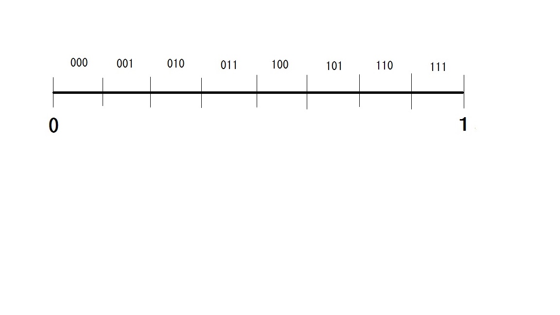
Figure 1: $\{0,1\}^{3}$ is identified with the set of 8 segments $\mathcal{I}_{3}$.

The $s$-dimensional hypercube $I^{s}$ is approximated by the set $\mathcal{I}_{n}^{s}$ of $2^{ns}$ hypercubes, which is identified with $I_{n}^{s}=({\mathbb{F}_{2}}^{n})^{s}=M_{s,n}({\mathbb{F}_{2}})=:V$. In sum,

Definition 1

Let $V:=M_{s,n}({\mathbb{F}_{2}})$ be the set of $(s\times n)$-matrices with coefficients in ${\mathbb{F}_{2}}=\{0,1\}$. An element $B=(b_{ij})\in V$ is identified with an $s$-dimensional hypercube in $\mathcal{I}_{n}^{s}$, consisting of elements $(x_{1},\ldots,x_{s})\in\mathbb{R}^{s}$ where, for each $i$, the binary expansion of $x_{i}$ coincides with $0.b_{i1}b_{i2}\cdots b_{in}$ up to the $n$-th digit below the decimal point. By abuse of the language, the notation $B$ is used for the corresponding hypercube.

Example 2

In the case $n=3$ and $s=2$, for example,

$$B=\left(\begin{array}[]{c}100\\ 011\end{array}\right)\mbox{ corresponds to }[0.100,0.101)\times[0.011,0.100).$$

As an approximation of $f:I^{s}\to\mathbb{R}$, define

$$f_{n}:\mathcal{I}_{n}^{S}=V\to\mathbb{R},\quad B\mapsto f_{n}(B):=\frac{1}{{{\mathrm{Vol}}}(B)}\int_{B}f\,\mathrm{d}x$$

by mapping a small hypercube $B$ of edge length $2^{-n}$ to the average of $f$ over this small hypercube. Thus, $f_{n}$ is the discretization (with $n$-bit precision) of $f$ by taking the average over each small hypercube.

In the following, we do not compute $f_{n}$, but consider as if we are given $f_{n}$. More precisely saying, let $\bm{x}_{B}$ denote the mid point of the hypercube $B$, and we approximate $f_{n}(B)$ by $f(\bm{x}_{B})$. For sufficiently large $n$, say, $n=32$, the approximation error $|f_{n}(B)-f(\bm{x}_{B})|$ (which we call the discretization error of $f$ at $B$ ) would be small enough: if $f$ is Lipschitz continuous, then the error has order $\sqrt{s}2^{-n}$.

From now on, we assume that $n$ is taken large enough, so that this discretization error is negligible in practice for the QMC integration considered. A justification is that we have only finite precision computation in digital computers, so a function $f$ has discretized domain with some finite precision. This assumption is somewhat cheating, but seems to work well in many practical uses.

By definition of the above discretization, we have an equality

$$\int_{[0,1)^{s}}f(x)\,\mathrm{d}x=\frac{1}{|V|}\sum_{B\in V}f_{n}(B).$$

2.2 Discrete Fourier transform

For $A,B\in V$, we define its inner product by

$$(A,B):=\mbox{trace}(^{t}AB)=\sum_{1\leq i\leq s,1\leq j\leq n}a_{ij}b_{ij}\in{\mathbb{F}_{2}}\quad(\bmod 2).$$

For a function $g:V\to\mathbb{R},$ its discrete Fourier transform $\hat{g}:V\to\mathbb{R}$ is defined by

$$\hat{g}(A):=\frac{1}{|V|}\sum_{B\in V}g(B)(-1)^{(B,A)}.$$

Thus

$$\hat{f_{n}}(0)=\frac{1}{|V|}\sum_{B\in V}f_{n}(B)=I(f).$$

Remark 1

The value $\hat{f_{n}}(A)$ coincides with the $A$-th Walsh coefficient of the function $f$ defined as follows. Let $A=(a_{ij})$. Define an integer $c_{i}:=\sum_{j=1}^{n}a_{ij}2^{j}$ for each $i=1,\ldots,s$. Then the $A$-th Walsh coefficient of $f$ is defined as the standard multi-indexed Walsh coefficient $\hat{f}_{c_{1},\ldots,c_{s}}$.

2.3 Digital nets, and QMC-error in terms of Walsh coefficients

Definition 2

Let $P\subset V$ be an ${\mathbb{F}_{2}}$-linear subspace (namely, $P$ is closed under componentwise addition modulo 2). Then, $P$ can be regarded as a set of small hypercubes in $\mathcal{I}_{n}^{s}$, or, a finite point set $\mathcal{P}\subset I^{s}$ by taking the mid point of each hypercubes. Such a point set $\mathcal{P}$ (or even $P$) is called a digital net with base 2.

This notion goes back to Sobol’ and Niederreiter; see for example (DICK-PILL-BOOK, , Definition 4.47). For such an ${\mathbb{F}_{2}}$-subspace $P$, let us define its perpendicular space by

$$P^{\perp}:=\{A\in V\ |\ (B,A)=0\ (\forall B\in P)\}.$$

QMC integration of $f_{n}$ by $P$ is by definition

$$I(f_{n};P):=\frac{1}{|P|}\sum_{B\in P}f_{n}(B)=\sum_{A\in P^{\perp}}\hat{f_{n}}(A),$$ (2)

where the right equality (called Poisson summation formula) follows from

$$\begin{array}[]{rcl}\sum_{A\in P^{\perp}}\hat{f_{n}}(A)&=&\sum_{A\in P^{\perp}}\frac{1}{|V|}(\sum_{B\in V}f_{n}(B)(-1)^{(B,A)})\\ &=&\frac{1}{|V|}\sum_{B\in V}f_{n}(B)\sum_{A\in P^{\perp}}(-1)^{(B,A)}\\ &=&\frac{1}{|V|}\sum_{B\in P}f_{n}(B)|P^{\perp}|\\ &=&\frac{1}{|P|}\sum_{B\in P}f_{n}(B).\\ \end{array}$$

2.4 Koksma-Hlawka type inequality by Dick

From (2), we have a QMC integration error bound by Walsh coefficients

$${{\mathrm{Error}}}(f_{n};P)=|I(f_{n};P)-\hat{f_{n}}(0)|\\ =\left|\sum_{A\in P^{\perp}-\{0\}}\hat{f_{n}}(A)\right|\leq\sum_{A\in P^{\perp}-\{0\}}|\hat{f_{n}}(A)|.\\$$ (3)

Thus, to bound the error, it suffices to bound $|\hat{f_{n}}(A)|$.

Theorem 2.1 (Decay of Walsh coefficients, Dick-Decay )

For an $n$-smooth function $f$, there is a notion of $n$-norm $||f||_{n}$ and a constant $C(s,n)$ independent of $f$ and $A$ with

$$|\hat{f_{n}}(A)|\leq C(s,n)||f||_{n}2^{-\mu(A)}.$$

(See (DICK-PILL-BOOK, , Theorem 14.23) for a general statement.) Here, $\mu(A)$ is defined as follows:

Definition 3

For $A=(a_{ij})_{1\leq i\leq s,1\leq j\leq n}\in V$, its Dick weight $\mu(A)$ is defined by

$$\mu(A):=\sum_{1\leq i\leq s,1\leq j\leq n}ja_{ij},$$

where $a_{ij}\in\{0,1\}$ are considered as integers (without modulo 2).

Example 3

In the case of $s=3,n=4$, for example,

$$A=\left(\begin{array}[]{c}1001\\ 0111\\ 0010\end{array}\right)\stackrel{{\scriptstyle ja_{ij}}}{{\to}}\left(\begin{array}[]{c}1004\\ 0234\\ 0030\end{array}\right)\to\mu(A)=\begin{array}[]{r}(1+0+0+4)\\ +(0+2+3+4)\\ +(0+0+3+0)\end{array}=17.$$

Walsh figure of merit of $P$ is defined as follows WAFOM :

Definition 4 (WAFOM)

Let $P\subset V$. WAFOM of $P$ is defined by

$${{\mathrm{WF}}}(P):=\sum_{A\in P^{\perp}-\{0\}}2^{-\mu(A)}.$$

By plugging this definition and Dick’s Theorem 2.1 into (3), we have an inequality of Koksma-Hlawka type:

$${{\mathrm{Error}}}(f_{n};P)\leq C(s,n)||f||_{n}{{\mathrm{WF}}}(P).$$ (4)

2.5 A toy experiment on ${{\mathrm{WF}}}(P)$

We shall see how WAFOM works for a toy case of $n=3$-digit precision and $s=1$ dimension. In Figure 1, the unit interval $I$ is divided into 8 intervals, each of which corresponds to a $(1\times 3)$-matrix in ${\mathbb{F}_{2}}^{3}=V$. Table1 lists the seven subspaces of dimension 2, selection of four of them, and their WAFOM and QMC error for the integrand $f(x)=x,x^{2}$ and $x^{3}$.

Table 1: Toy examples for WAFOM for 3-digit discretization for integrated $x,x^{2}$ and $x^{3}$

$$\begin{array}[]{rccccccl}V=\{000&001&010&011&100&101&110&111\}\\ (100)^{\perp}=\{000&001&010&011&\phantom{000}&\phantom{000}&\phantom{000}&\phantom{000}\}\\ (010)^{\perp}=\{000&001&\phantom{000}&\phantom{000}&100&101&\phantom{000}&\phantom{000}\}\\ (110)^{\perp}=\{000&001&\phantom{000}&\phantom{000}&\phantom{000}&\phantom{000}&110&111\}\\ (001)^{\perp}=\{000&\phantom{000}&010&\phantom{000}&100&\phantom{000}&110&\phantom{000}\}\\ (101)^{\perp}=\{000&\phantom{000}&010&\phantom{000}&\phantom{000}&101&\phantom{000}&111\}\\ (011)^{\perp}=\{000&\phantom{000}&\phantom{000}&011&100&\phantom{000}&\phantom{000}&111\}\\ (111)^{\perp}=\{000&\phantom{000}&\phantom{000}&011&\phantom{000}&101&110&\phantom{000}\}\\ \end{array}$$

$P$	$\begin{array}[]{l}\mu(A)\mbox{ for}\\ A\in P^{\perp}\setminus 0\end{array}$	WF($P$)	Error for $x$	Error for $x^{2}$	Error for $x^{3}$
$V$	$\emptyset$	0	0	$-$0.0013	$-$0.0020
$001^{\perp}$	0+0+3	$2^{-3}$	$-$0.0625	$-$0.0638	$-$0.0637
$101^{\perp}$	1+0+3	$2^{-4}$	0	$-$0.0299	$-$0.0449
$011^{\perp}$	0+2+3	$2^{-5}$	0	+0.0143	+0.0215
$111^{\perp}$	1+2+3	$2^{-6}$	0	$-$0.0013	$-$0.0137

The first line in Table 1 shows the 8-element set $V={\mathbb{F}_{2}}^{3}$, corresponding to the 8 intervals in Figure 1. The next line $(100)^{\perp}$ denotes the 2-dimensional subspace of $V$ consisting of the elements perpendicular to $(100)$, that is, the four vectors whose first digit is 0. In the same manner, all 2-dimensional subspaces of $V$ are listed. The last one is $(111)^{\perp}$, consisting of the four vectors $(x_{1},x_{2},x_{3})$ with $x_{1}+x_{2}+x_{3}=0(\bmod 2)$.

Our aim is to decide which is the best (or most “uniform”) among the seven 2-dimensional sub-vector spaces for QMC integration. Intuitively, $(100)^{\perp}$ is not a good choice since all the four intervals cluster in $[0,1/2]$. Similarly, we exclude $(010)^{\perp}$ and $(110)^{\perp}$. We compare the remaining four candidates by two methods: computing WAFOM, and computing QMC integration errors with test integrand functions $x,x^{2}$ and $x^{3}$.

The results are shown in the latter part of Table 1. The first line corresponds to the case of $P=V$. Since $P^{\perp}-\{0\}$ is empty, ${{\mathrm{WF}}}(P)=0$. For the remaining four cases $P=(x_{1},x_{2},x_{3})^{\perp}$, note that $\{(x_{1},x_{2},x_{3})^{\perp}\}^{\perp}=\{(000),(x_{1},x_{2},x_{3})\}$ and $P^{\perp}-\{0\}=\{(x_{1},x_{2},x_{3})\}$, thus we have ${{\mathrm{WF}}}(P)=2^{-\mu((x_{1},x_{2},x_{3}))}.$ The third column in the latter table shows WAFOM for five different choices of $P$. The three columns “Error for $x^{i}$” with $i=1,2,3$ show the QMC integration error by $P$ for integrating $x^{i}$ over $[0,1]$. We used the mid point of each segment (of length 1/8) to evaluate $f$. Thus, the listed errors include both the discretization errors and QMC-integration errors for $f_{n}$. For the first line, $P=V$ implies no QMC integration error for $f_{n}$ ($n=3$), so the values show the discretization error exactly. The error bound (4) is proportional to ${{\mathrm{WF}}}(P)$ for a fixed integrand. The table shows that, for these test functions, the actual errors are well reflected in WAFOM values.

Here is a loose interpretation of ${{\mathrm{WF}}}(P)$. For an ${\mathbb{F}_{2}}$-linear $P$,

• $A\in P^{\perp}\setminus\{0\}$ is a linear relation satisfied by $P$.

• $\mu(A)$ measures “complexity” of $A$.

• ${{\mathrm{WF}}}(P)=\sum_{A\in P^{\perp}\setminus\{0\}}2^{-\mu(A)}$ is small if all relations have high complexity, and hence $P$ is close to “uniform.”

The weight $j$ in the sum $\sum ja_{ij}$ in the definition of $\mu(A)$ denotes that the $j$-th digit below the decimal point is counted with complexity $2^{-j}$.

3 Point sets with low WAFOM values

3.1 Existence and non-existence of low WAFOM point sets

Theorem 3.1

There are absolute (i.e. independent of $s,n$ and $d$) positive constants $C,D,E$ such that for any positive integer $s,n$ and $d\geq 9s$, there exists a $P\subset V$ of ${\mathbb{F}_{2}}$-dimension $d$ (hence cardinality $N=2^{d}$) satisfying

$$\begin{array}[]{rlc}{{\mathrm{WF}}}(P)&\leq&E\cdot 2^{-Cd^{2}/s+Dd}=E\cdot N^{-C\log_{2}N/s+D}.\end{array}$$

Since the exponent $-C\log_{2}N/s+D$ goes to $-\infty$ when $N\to\infty$, this shows that there exist point sets with “higher order convergence” having this order of WAFOM. There are two independent proofs: M-Yoshiki YOSHIKI-MATSUMOTO shows the positivity of the probability to have low-WAFOM point sets under a random choice of its basis (hence non-constructive), and K.Suzuki SUZUKI2012 shows a construction using Dick’s interleaving method (DICK-PILL-BOOK, , §15) for Niederreiter-Xing sequence niederreiter:xing . Suzuki SUZUKI2014 generalizes YOSHIKI-MATSUMOTO and YOSHIKI2014 for arbitrary base $b$. Theorem 3.1 is similar to the Dick’s construction of point sets with $W_{\alpha}(\mathcal{P})=O(N^{-\alpha}(logN)^{s\alpha})$ for arbitrary high $\alpha\geq 1$, but there seems no implication between his result and this theorem.

On the other side, Yoshiki YOSHIKI2014 proved the following theorem that the order of the exponent $d^{2}/s$ is sharp, namely, WAFOM can not be so small:

Theorem 3.2

Let $C^{\prime}>1/2$ be any constant. For any positive integer $s,n$ and $d\geq s\times(\sqrt{C^{\prime}+1/16}+3/4)/(C^{\prime}-1/2)$, any linear subspace $P\subset V$ of ${\mathbb{F}_{2}}$-dimension $d$ satisfies

$$\begin{array}[]{rlc}{{\mathrm{WF}}}(P)&\geq&2^{-C^{\prime}d^{2}/s}.\\ \end{array}$$

3.2 An efficient computation method of WAFOM

Since $P$ is intended for a QMC integration where the enumeration of $P$ is necessary, $|P|=2^{\dim_{{\mathbb{F}_{2}}}P}$ can not be huge. On the other hand, $|V|=2^{ns}$ would be huge, say, for $n=32$ and $s>2$. Since $\dim_{{\mathbb{F}_{2}}}P+\dim_{{\mathbb{F}_{2}}}P^{\perp}=\dim_{{\mathbb{F}_{2}}}V$, $|P^{\perp}|$ must be huge. Thus, a direct computation of ${{\mathrm{WF}}}(P)$ using Definition 4 would be too costly. In WAFOM , the following formula is given by a Fourier inversion. Put $B=(b_{i,j})$, then we have

$${{\mathrm{WF}}}(P)=\frac{1}{|P|}\sum_{B\in P}\left\{\prod_{1\leq i\leq s,1\leq j\leq n}[(1+(-1)^{b_{i,j}}2^{-j})]-1\right\}.$$

This is computable in $O(nsN)$ steps of arithmetic operations in real numbers, where $N=|P|$. Compared with most of other discrepancies, this is relatively easily computable. This allows us to do a random search for low-WAFOM point sets.

Remark 2

1. The above equality holds only for an ${\mathbb{F}_{2}}$-linear $P$. Since the left hand side is non-negative, so is the right sum in this case. It seems impossible to define WAFOM for a general point set by using this formula, since for a general (i.e. non-linear) $P$, the sum at the right hand side is sometimes negative and thus will never give a bound on the integration error.

2. The right sum may be interpreted as the QMC integration of a function (whose definition is given in the right hand side of the equality) by $P$. The integration of the function over total space $V$ is zero. Hence, the above equality indicates that, to have a best ${\mathbb{F}_{2}}$-linear $P$ from the viewpoint of WAFOM, it suffices to have a best $P$ for QMC integration for a single specified function. This is in contrast to the definition of star-discrepancy, where all the rectangle characteristic functions are used as the test functions, and the supremum of their QMC integration errors is taken.

3. Harase-OhoriHARASE-OHORI gives a method to accelerate this computation by a factor of 30, using a look-up table. Ohori-YoshikiOHORI-YOSHIKI gives a faster and simpler method to compute a good approximation of WAFOM, using that Walsh coefficients of exponential function approximates the Dick weight $\mu$. More precisely, ${{\mathrm{WF}}}(P)$ is well-approximated by the QMC-error of the function $\exp(-2\sum_{i=1}^{s}x_{i})$, whose value is easy to evaluate in modern CPUs.

4 Experimental results

4.1 Random search for low WAFOM point sets

We fix the precision $n=30$. We consider two cases of the dimension $s=4$ and $s=8$. For each $d=8,9,10,\ldots,16$, we generate $d$-dimensional subspace $P\subset V=({\mathbb{F}_{2}}^{30})^{s}$ 10000 times, by the uniformly random choice of $d$ elements as its basis. Let $P_{d,s}$ be the point set with the lowest WAFOM among them. For the comparison, $Q_{d,s}$ be the point set of the 100th lowest WAFOM.

4.2 Comparison of QMC rules by WAFOM

For a comparison, we use two other QMC quadrature rules, namely, Sobol’ sequence improved by Joe and Kuo JOE-KUO , and Niederreiter-Xing sequence (NX) implemented by Pirsic PIRSIC and by Dirk Nuyens (NUYENS, , item nxmats) (downloaded from the latter). Figure 2 shows the WAFOM values for these four kinds of point sets, with size $2^{8}$ to $2^{16}$.

Figure 2: WAFOM values for: (1) best WAFOM among 10000, (2) the 100th best WAFOM, (3) Niederreiter-Xing, (4) Sobol’, of size $2^{d}$ with $d=8,9,\ldots,16$. The vertical axis is for $\log_{2}$ of their WAFOM, and the horizontal for $\log_{2}$ of the size of point sets. The left figure is for dimension $s=4$, the right $s=8$.

For $s=4$, Sobol’ has largest WAFOM value, while NX has small WAFOM comparable to the 100th best $Q_{d,s}$ selected by WAFOM. In $d=14$, NX has much larger WAFOM than that of $Q_{14,s}$, while in $d=15$ the converse occurs. Note that this seems to be reflected in the following experiments. For $s=8$, the four kinds of point sets show small differences in values of their WAFOM. Indeed, NX has smaller WAFOM value than the best point set among randomly generated 10000 for each $d$, while Sobol’ has larger WAFOM values. A mathematical analysis on this good grade of NX would be interesting.

4.3 Comparison by numerical integration

In addition to the above four kinds of QMC rules, Monte Carlo method is used for comparison (using Mersenne Twister MT pseudorandom number generator). For the test functions, we use 6 Genz functions GENZ1987 :

Oscillatory

$f_{1}(\bm{x})=\cos(2\pi u_{1}+\sum_{i=1}^{s}a_{i}x_{i})$,

Product Peak

$f_{2}(\bm{x})=\prod_{i=1}^{s}[1/(a_{i}^{2}+(x_{i}-u_{i})^{2})]$,

Corner Peak

$f_{3}(\bm{x})=(1+\sum_{i=1}^{s}a_{i}x_{i})^{-(s+1)}$

Gaussian

$f_{4}(\bm{x})=\exp(-\sum_{i=1}^{s}a_{i}^{2}(x_{i}-u_{i})^{2})$

Continuous

$f_{5}(\bm{x})=\exp(-\sum_{i=1}^{s}a_{i}|x_{i}-u_{i}|)$

Discontinuous

$f_{6}(\bm{x})=\begin{cases}0&\mbox{ if }x_{1}>u_{1}\mbox{ or }x_{2}>u_{2},\\ \exp(\sum_{i=1}^{s}a_{i}x_{i}))&\mbox{otherwise.}\end{cases}$

This selection is copied from (NOVAK-RITTER, , P.91) HARASE-OHORI . The parameters $a_{1},\ldots,a_{s}$ are selected so that (1) they are in an arithmetic progression (2) $a_{s}=2a_{1}$ (3) the average of $a_{1},\ldots,a_{s}$ coincides with the average of $c_{1},\ldots,c_{10}$ in (NOVAK-RITTER, , Equation (10)) for each test function. The parameters $u_{i}$ are generated randomly by MT .

Figure 3: QMC integration errors for (1) best WAFOM among 10000, (2) the 100th best WAFOM, (3) Niederreiter-Xing, (4) Sobol’, (5) Monte Carlo, using six Genz functions on the 4-dimensional unit cube. The vertical axis is for $\log_{2}$ of the errors, and the horizontal for $\log_{2}$ of the size of point sets. The error is the mean square error for 100 randomly digital shifted point sets.

Figure 3 shows the QMC integration errors for six test functions with five methods, for dimension $s=4$. The error for Monte Carlo is of order $N^{-1/2}$. The best WAFOM point sets (WAFOM) and Niederreiter-Xing (NX) are comparable. For the function Oscillatory, where its higher derivatives grow relatively slowly, WAFOM point sets perform better than NX and Sobol’, and the convergence rate seems of order $N^{-2}$. For Product peak and Gaussian, WAFOM and NX are comparable; this coincides with the fact that higher derivatives of these test functions rapidly grow, but still we observe convergence rate $N^{-1.6}$. For Corner peak, WAFOM performs better than NX. It is somewhat surprising that the convergence rate is almost $N^{-1.8}$ for WAFOM point sets. For Continuous, NX performs better than WAFOM. Since the test functions are not differentiable, $||f||_{n}$ is unbounded and hence the inequality (4) has no meaning. Still, for Continuous, the convergence rate of WAFOM is almost $N^{-1.2}$. For Discontinuous, NX and Sobol’ perform better than WAFOM. Note that except Discontinuous, the large/small value of WAFOM of NX for $d=14,15$ observed in the left of Figure 2 seems to be reflected in the five graphs.

We conducted similar experiments for $s=8$ dimension, but we omit the results, since their difference in WAFOM is small, and the QMC rules show not much difference. We report that still we observe convergence rate with $N^{-\alpha}$ with $\alpha>1.05$ for the five test functions except Discontinuous, for WAFOM selected points and NX.

Remark 3

1. Convergence rate for the integration error is even faster than that of WAFOM values, for WAFOM selected point sets and NX for $s=4$, while Sobol’ sequence converging with rate $N^{-1}$. We feel that these go against our intuition, so checked the code and compared with MC. We do not know why NX and WAFOM work so well.

2. As a referee pointed out, it is hard to observe converging rate $N^{-C\log_{2}N/s+D}$ in Theorem 3.1 from the graphs.

5 WAFOM versus other figure of merits

Niederreiter’s $t$-value niederreiter:book is a most established figure of merit of a digital net. Using test functions, we compare the effect of $t$-value and WAFOM for QMC integration.

5.1 $t$-value

Let $\mathcal{P}\subset I^{S}=[0,1)^{s}$ be a finite set of cardinality $2^{m}$. Let $n_{1},n_{2},\ldots,n_{s}\geq 0$ be integers. Recall that $\mathcal{I}_{n_{i}}$ is the set of $2^{n_{i}}$ intervals partitioning $I$. Then, $\prod_{i=1}^{s}\mathcal{I}_{n_{i}}$ is a set of $2^{n_{1}+n_{2}+\cdots+n_{s}}$ intervals. We want to make the QMC integration error 0 in computing the volume of every such interval. A trivial bound is $n_{1}+n_{2}+\cdots+n_{s}\leq m$, since at least one point must fall in each interval. The point set $\mathcal{P}$ is called a $(t,m,s)$-net if the QMC integration error for each interval is zero, for any tuple $(n_{1},\ldots,n_{s})$ with

$$n_{1}+n_{2}+\cdots+n_{s}\leq m-t.$$

Thus, smaller $t$-value is more preferable.

5.2 Experiments on WAFOM versus $t$-value

We fix the dimension $s=4$ and the precision $n=32$, and generate $10^{6}$ (${\mathbb{F}_{2}}$-linear) point sets of cardinality $2^{12}$ by uniform random choices of their ${\mathbb{F}_{2}}$ basis consisting of 12 vectors. We sort these $10^{6}$ point sets, according to their $t$-values. It turns out that $3\leq t\leq 12$, and the frequency of the point sets for a given $t$-value is as follows.

$t$	3	4	5	6	7	8	9	10	11	12
freq.	63	6589	29594	32403	18632	8203	2994	1059	365	98

Then, we sort the same $10^{6}$ point sets by WAFOM. We categorize them into 10 classes from the smallest WAFOM, so that $i$-th class has the same frequency with the $i$-th class by $t$-value. Thus, the same $10^{6}$ point sets are categorized in two ways. For a given test integrand function, compute the mean square error of QMC integral in each category, for those graded by $t$-value and those graded by WAFOM.

Figure 4: Left: Hellekalek’s function $f(\bm{x})=(x_{1}^{1.1}-\frac{1}{1+1.1})(x_{2}^{1.7}-\frac{1}{1+1.7})(x_{3}^{2.3}-\frac{1}{1+2.3})(x_{4}^{2.9}-\frac{1}{1+2.9})$, right: Hamukazu’s function $f(\bm{x})=2^{4}\{5x_{1}\}\{7x_{2}\}\{11x_{3}\}\{13x_{4}\}$, where $\{x\}:=x-[x]$. Horizontal axis for category, vertical for the $\log_{2}$ of error. $\Box$:WAFOM, $+\times$:$t$-value.

Figure 4 shows $\log_{2}$ of the mean square integration error, for each category corresponding to $3\leq t\leq 12$ for $t$-value ($+\times$), and for the category sorted by WAFOM value ($\Box$). The smooth test function in the left hand side comes from Hellekalek HELEKALLEK1998 , and the non-continuous function in the right hand side was communicated from Kimikazu Kato (refered to as “Hamukazu” according to his established twitter handle). From the left figure, for $t=3$, the average error for the best 63 point sets with the smallest $t$-value 3 is much larger than the average from the best 63 point sets selected by WAFOM. Thus, the experiments show that for this test function, WAFOM seems to work better than $t$-value in selecting good point set. We have no explanation why the error decreases for $t\geq 9$. In the right figure, for Hamukazu’s non-continuous test function, $t$-value works better in selecting good points.

Thus, it is expected that digital nets that have small $t$-value and small WAFOM would work well for smooth functions and robust to non-smooth functions. Harase HARASE-HYBRID noticed that Owen linear scrambling (DICK-PILL-BOOK, , §13)OWEN-SCRAMBLING preserves $t$-value, but changes WAFOM. Starting from a Niederreiter-Xing sequence with small $t$, he applied Owen linear scrambling to find a point set with low WAFOM and small $t$-value. He obtained good results for wide range of integrands.

5.3 Dick’s $\mu_{\alpha}$, and non-discretized case

Let $\alpha>0$ be an integer. For $A\in M_{S,n}({\mathbb{F}_{2}})$, the Dick’s $\alpha$-weight $\mu_{\alpha}(A)$ is defined as follows. It is a part of summation appeared in Definition 3 of $\mu(A)$: the sum is taken up to $\alpha$ nonzero entries from the right in each row.

Example 4

Suppose $\alpha=2$.

$$A=\begin{array}[]{c}1001\\ 0111\\ 0010\end{array}\stackrel{{\scriptstyle ja_{ij}}}{{\to}}\begin{array}[]{c}\mathbf{1}00\mathbf{4}\\ 02\mathbf{3}\mathbf{4}\\ 00\mathbf{3}0\end{array}\to\mu_{\alpha}(A)=\begin{array}[]{r}(1+0+0+4)\\ +(0+0+3+4)\\ +(0+0+3+0)\end{array}=15.$$

For ${\mathbb{F}_{2}}$-linear $P\subset M_{S,n}({\mathbb{F}_{2}})$,

$$W_{\alpha}(P):=\sum_{A\in P^{\perp}-\{0\}}2^{-\mu_{\alpha}(A)}.$$ (5)

To be precise, we need to take $n\to\infty$, as follows. We identify $I=[0,1]$ with the product $W:={\mathbb{F}_{2}}^{\mathbb{N}}$ via binary fractional expansion (neglecting a measure-zero set). Let $K:={\mathbb{F}_{2}}^{\oplus\mathbb{N}}\subset W$ be the subspace consisting of vectors with finite number of nonzero components (this is usually identified with $\mathbb{N}\cup\{0\}$ via binary expansion and reversing the digits). We define inner product $W\times K\to{\mathbb{F}_{2}}$ as usual. Then, for a finite subgroup $P\subset W^{s}$, its perpendicular space $P^{\perp}\subset K^{s}$ is defined and is countable. For $A\in K^{s}$, $\mu_{\alpha}(A)$ is analogously defined, and the right hand side of (5) is absolutely converging. Dick Dick-Decay proved

$${{\mathrm{Error}}}(f;P)\leq C(s,\alpha)||f||_{\alpha}W_{\alpha}(P),$$

and constructed a sequence of $P$ with $W_{\alpha}(P)=O(N^{-\alpha}(\log N)^{S\alpha})$ called higher order digital nets. (See DICK-PILL-BOOK for a comprehensive explanation.) Existence results and search algorithms for higher order polynomial lattice rules are studied in BARDEAUX-DICK DICK-KRITZER-PILL-SCH .

WAFOM is an $n$-digit discretized version of $W_{\alpha}$ where $\alpha=n$. WAFOM loses freedom to choose $\alpha$, but it might be a merit since we do not need to choose $\alpha$.

Remark 4

In Dick’s theory, $\alpha$ is fixed. In fact, setting $\alpha=\log N$ does not yield useful bound, since $C(s,\log N)W_{\log N}(P)\to\infty\ (N\to\infty)$.

The above experiments show that, to have a small QMC-error by low WAFOM point sets, the integrand should have high order partial derivatives with small norms (see a preceding research HARASE-OHORI , too). However, WAFOM seems to work with some non-differentiable functions (such as Continuous in the previous section).

5.4 $t$-value again

Niederreiter-Pirsic NIEDERREITER-PIRSIC showed that for a digital net $P$, the strict $t$-value of $P$ as a $(t,m,s)$-net is expressed as

$$m-t+1=\min_{A\in P^{\perp}-\{0\}}\mu_{1}(A).$$ (6)

Here $\mu_{1}$ is Dick’s $\alpha$-weight for $\alpha=1$, which is known as the Niederreiter-Rosenbloom-Tsfasman weight.

There is a strong resemblance between (6) and Definition 4. Again in (6), high complexity of all elements in $P^{\perp}-\{0\}$ gives strong uniformity (i.e., small $t$-value). The right hand side of (6) is efficiently computable by a MacWilliams-type identity in $O(sN\log N)$ steps of integer operation DICK-MATSUMOTO .

Question 1

The formula (6) for $t$-value uses the minimum over $P$, while Definition 4 of WAFOM and (5) use the summation over $P$. Can we connect $t$-value in (6) with WAFOM in Definition 4? It may perhaps relate with ultra-discretization ULTRA-DISCRETIZATION .

6 Randomization by digital shift

Let $P\subset M_{s,n}({\mathbb{F}_{2}})$ be a linear subspace. Choose $\sigma\in M_{s,n}({\mathbb{F}_{2}})$. The point set $P+\sigma:=\{B+\sigma|B\in P\}$ is called the digital shift of $P$ by $\sigma$. Since $P+\sigma$ is not an ${\mathbb{F}_{2}}$-linear subspace, one can not define ${{\mathrm{WF}}}(P+\sigma)$. Nevertheless, the same error bound holds as $P$. Under a uniform random choice of $\sigma$, $P+\sigma$ becomes unbiased. Moreover, the mean square error is bounded as follows:

Theorem 6.1

(Goda-Ohori-Suzuki-Yoshiki GOSY )

$${{\mathrm{Error}}}(f_{n};P+\sigma)\leq C(s,n)||f||_{n}{{\mathrm{WF}}}(P),\mbox{ and}$$

$$\sqrt{{\mathbb{E}}({{\mathrm{Error}}}(f_{n};P+\sigma)^{2})}\leq C(s,n)||f||_{n}{{\mathrm{WF}}}^{\mbox{r.m.s.}}(P),$$

$$\mbox{where }{{\mathrm{WF}}}^{\mbox{r.m.s.}}(P):=\sqrt{\sum_{A\in P^{\perp}-\{0\}}2^{-{2}\mu(A)}}.$$

7 Variants of WAFOM

As mentioned in the previous section, GOSY defined ${{\mathrm{WF}}}^{\mbox{r.m.s.}}(P)$. As another direction, the following generalization of WAFOM is proposed by Yoshiki YOSHIKIBOUND and Ohori OHORI-MASTER : in Definition 3, the function $\mu(A)$ might be generalized by:

$$\mu_{\delta}(A):=\sum_{1\leq i\leq s,1\leq j\leq n}(j+\delta)a_{ij}$$

for any (even negative) real number $\delta$ (note that this definition is different from that of $\mu_{\alpha}$, but we could not find a better notation). Then Definition 4 gives ${{\mathrm{WF}}}_{\delta}(P)$. The case where $\delta=1$ is dealt in YOSHIKIBOUND . A weak point of the original WAFOM is that WAFOM value does not vary enough and consequently it is not useful in grading point sets for a large $s$, see Figure 2, the $s=8$ case. By choosing a suitable $\delta$, we obtain ${{\mathrm{WF}}}_{\delta}(P)$ that varies for large $s$ (even for $s=16$) and useful in choosing a good point set OHORI-MASTER . A table of bases of such point sets is available from Ohori’s GitHub Pages: http://majiang.github.io/qmc/index.html. These point sets are obtained by Ohori, using Harase’s method based on linear scrambling, from NX sequences. Thus, they have small $t$-values and small WAFOM values. Experiments show their good performance MORI-MULTI .

8 Conclusion

Walsh figure of merit (WAFOM) WAFOM for ${\mathbb{F}_{2}}$-linear point sets as a quality measure for a QMC rule is discussed. Since WAFOM satisfies a Koksma-Hlawka type inequality (4), its effectiveness for very smooth functions is assured. Through the experiments on QMC integration, we observed that the low WAFOM point sets show higher order convergence such as $O(N^{-1.2})$ for several test functions (including non-smooth one) in dimension four, and $O(N^{-1.05})$ for dimension eight.

- (1) Bardeaux, J., Dick, J., Leobacher, G., Nuyens, D., Pillichshammer, F.: Efficient calculation of the worst-case error and (fast) component-by-component construction of higher order polynomial lattice rules. Numer. Algorithms 59, 403–431 (2012)
- (2) Dick, J.: Walsh spaces containing smooth functions and quasi-monte carlo rules of arbitrary high order. SIAM J. Numer. Anal. 46, 1519–1553 (2008)
- (3) Dick, J.: The decay of the walsh coefficients of smooth functions. Bull. Austral. Math. Soc. 80, 430–453 (2009)
- (4) Dick, J.: On quasi-Monte Carlo rules achieving higher order convergence. In: Monte Carlo and Quasi-Monte Carlo Methods 2008, pp. 73–96. Springer (2009)
- (5) Dick, J., Kritzer, P., Pillichshammer, F., Schmid, W.: On the existence of higher order polynomial lattices based on a generalized figure of merit. J. Complex 23, 581–593 (2007)
- (6) Dick, J., Matsumoto, M.: On the fast computation of the weight enumerator polynomial and the value of digital nets over finite abelian groups. SIAM J. Discrete Math. 27, 1335–1359 (2013)
- (7) Dick, J., Pillichshammer, F.: Digital Nets and Sequences. Discrepancy Theory and Quasi-Monte Carlo Integration. Cambridge University Press, Cambridge (2010)
- (8) Genz, A.: A package for testing multiple integration subroutines. In: Numerical Integration: Recent Developments, Software and Applications, pp. 337–340. Springer (1987)
- (9) Goda, T., Ohori, R., Suzuki, K., Yoshiki, T.: The mean square quasi-Monte Carlo error for digitally shifted digital nets. ArXiv:1412.0783
- (10) Harase, S.: Quasi-Monte Carlo point sets with small t-values and WAFOM. Applied Mathematics and Computation 254, 318–326 (2015). ArXiv:1406.1967
- (11) Harase, S., Ohori, R.: A search for extensible low-WAFOM point sets. ArXiv:1309.7828
- (12) Hellekalek, P.: On the assessment of random and quasi-random point sets. In: Random and Quasi-Random Point Sets, pp. 49–108. Springer (1998)
- (13) Joe, S., Kuo, F.: Constructing sobol’ sequences with better two-dimensional projections. SIAM J. Sci. Comput. 30, 2635–2654 (2008). URL http://web.maths.unsw.edu.au/~fkuo/sobol/new-joe-kuo-6.21201
- (14) Kakei, S.: Development in discrete integrable systems - ultra-discretization, quantization. RIMS, Kyoto, Japan (2001)
- (15) Matsumoto, M., Nishimura, T.: Mersenne twister: A 623-dimensionally equidistributed uniform pseudorandom number generator. ACM Trans. on Modeling and Computer Simulation 8(1), 3–30 (1998). http://www.math.sci.hiroshima-u.ac.jp/~m-mat/MT/emt.html
- (16) Matsumoto, M., Saito, M., Matoba, K.: A computable figure of merit for quasi-Monte Carlo point sets. Math. Comp. 83, 1233–1250 (2014)
- (17) Matsumoto, M., Yoshiki, T.: Existence of Higher Order Convergent Quasi-Monte Carlo Rules via Walsh Figure of Merit. In: Monte Carlo and Quasi-Monte Carlo Methods 2012, pp. 569–579. Springer (2013)
- (18) Mori, S.: A fast qmc computation by low-wafom point sets. In preparation
- (19) Niederreiter, H.: Random Number Generation and Quasi-Monte Carlo Methods. CBMS-NSF, Philadelphia, Pennsylvania (1992)
- (20) Niederreiter, H., Pirsic, G.: Duality for digital nets and its applications. Acta Arith. 97, 173–182 (2001)
- (21) Niederreiter, H., Xing, C.P.: Low-discrepancy sequences and global function fields with many rational places. Finite Fields and Their Applications 2, 241–273 (1996)
- (22) Novak, E., Ritter, K.: High-dimensional integration of smooth functions over cubes. Numer. Math. 75, 79–97 (1996)
- (23) Nuyens, D.: The magic point shop of qmc point generators and generating vectors. URL http://people.cs.kuleuven.be/~dirk.nuyens/qmc-generators/. Home page
- (24) Ohori, R.: Efficient quasi-monte carlo integration by adjusting the derivation-sensitivity parameter of walsh figure of merit (2015). Master’s Thesis
- (25) Ohori, R., Yoshiki, T.: Walsh figure of merit is efficiently approximable. In preparation
- (26) Owen, A.B.: Randomly permuted -nets and -sequences. In: Monte Carlo and Quasi-Monte Carlo Methods 1994, pp. 299–317. Springer (1995)
- (27) Pirsic, G.: A software implementation of niederreiter-xing sequences. In: Monte Carlo and quasi-Monte Carlo methods, 2000 (Hong Kong), pp. 434–445 (2002)
- (28) Suzuki, K.: An explicit construction of point sets with large minimum Dick weight. Journal of Complexity 30, 347–354 (2014)
- (29) Suzuki, K.: WAFOM on abelian groups for quasi-Monte Carlo point sets. Hiroshima Mathematical Journal (2015). To appear. arXiv:1403.7276
- (30) Yoshiki, T.: Bounds on walsh coefficients by dyadic difference and a new Koksma-Hlawka type inequality for quasi-monte carlo integration quasi-Monte Carlo integration. ArXiv:1504.03175
- (31) Yoshiki, T.: A lower bound on WAFOM. Hiroshima Mathematical Journal 44, 261–266 (2014)