Locality of connective constants

Abstract.

The connective constant $\mu(G)$ of a quasi-transitive graph $G$ is the exponential growth rate of the number of self-avoiding walks from a given origin. We prove a locality theorem for connective constants, namely, that the connective constants of two graphs are close in value whenever the graphs agree on a large ball around the origin (and a further condition is satisfied). The proof is based on a generalized bridge decomposition of self-avoiding walks, which is valid subject to the assumption that the underlying graph is quasi-transitive and possesses a so-called unimodular graph height function.

1. Introduction, and summary of results

There is a rich theory of interacting systems on infinite graphs. The probability measure governing a process has, typically, a continuously varying parameter, $z$ say, and there is a singularity at some ‘critical point’ $z_{\text{\rm c}}$. The numerical value of $z_{\text{\rm c}}$ depends in general on the choice of underlying graph $G$, and a significant part of the associated literature is directed towards estimates of $z_{\text{\rm c}}$ for different graphs. In most cases of interest, the value of $z_{\text{\rm c}}$ depends on more than the geometry of some bounded domain only. This observation provokes the question of ‘locality’: to what degree is the value of $z_{\text{\rm c}}$ determined by the knowledge of a bounded domain of $G$?

The purpose of the current paper is to present a locality theorem (namely, Theorem 5.1) for the connective constant $\mu(G)$ of the graph $G$. A self-avoiding walk (SAW) is a path that visits no vertex more than once. SAWs were introduced in the study of long-chain polymers in chemistry (see, for example, the 1953 volume of Flory, [14]), and their theory has been much developed since (see the book of Madras and Slade, [28], and the recent review [2]). If the underlying graph $G$ has some periodicity, the number of $n$-step SAWs from a given origin grows exponentially with some growth rate $\mu(G)$ called the connective constant of the graph $G$.

There are only few graphs $G$ for which the numerical value of $\mu(G)$ is known exactly (detailed references for a number of such cases may be found in [17]), and a substantial part of the literature on SAWs is devoted to inequalities for $\mu(G)$. The current paper may be viewed in this light, as a continuation of the series of papers on the broad topic of connective constants of transitive graphs by the same authors, see [15, 16, 17, 20].

The main result (Theorem 5.1) of this paper is as follows. Let $G$, $G^{\prime}$ be infinite, vertex-transitive graphs, and write $S_{K}(v,G)$ for the $K$-ball around the vertex $v$ in $G$. If $S_{K}(v,G)$ and $S_{K}(v^{\prime},G^{\prime})$ are isomorphic as rooted graphs, then

(1.1) $$|\mu(G)-\mu(G^{\prime})|\leq\epsilon_{K}(G),$$

where $\epsilon_{K}(G)\to 0$ as $K\to\infty$. (A related result holds for quasi-transitive graphs.) This is proved subject to certain conditions on the graphs $G$, $G^{\prime}$, of which the primary condition is that they support so-called ‘unimodular graph height functions’ (see Section 3 for the definition of a graph height function). The existence of unimodular graph height functions permits the use of a ‘bridge decomposition’ of SAWs (in the style of the work of Hammersley and Welsh [24]), and this leads in turn to computable sequences that converge to $\mu(G)$ from above and below, respectively. The locality result of (1.1) may be viewed as a partial answer to a question of Benjamini, [3, Conj. 2.3], made independently of the work reported here.

A class of vertex-transitive graphs of special interest is provided by the Cayley graphs of finitely generated groups. Cayley graphs have algebraic as well as geometric structure, and this allows a deeper investigation of locality and of graph height functions. The corresponding investigation is reported in the companion paper [18] where, in particular, we present a method for the construction of a graph height function via a suitable harmonic function on the graph.

The locality question for percolation was approached by Benjamini, Nachmias, and Peres [4] for tree-like graphs. Let $G$ be vertex-transitive with degree $d+1$. It is elementary that the percolation critical point satisfies $p_{\text{\rm c}}\geq 1/d$ (see [7, Thm 7]), and an asymptotically equivalent upper bound for $p_{\text{\rm c}}$ was developed in [4] for a certain family of graphs which are (in a certain sense) locally tree-like. In recent work of Martineau and Tassion [29], a locality result has been proved for percolation on abelian graphs. The proof extends the methods and conclusions of [21], where it is proved that the slab critical points converge to $p_{\text{\rm c}}({\mathbb{Z}}^{d})$, in the limit as the slabs become infinitely ‘fat’. (A related result for connective constants is included here at Example 5.3.)

We are unaware of a locality theorem for the critical temperature $T_{\text{\rm c}}$ of the Ising model. Of the potentially relevant work on the Ising model to date, we mention [6, 8, 10, 11, 26, 31].

This paper is organized as follows. Relevant background and notation is described in Section 2. The concept of a graph height function  is presented in Section 3, where examples are included of infinite graphs with graph height functions. Bridges and the bridge constant are defined in Section 4, and it is proved in Theorem 4.3 that the bridge constant equals the connective constant whenever there exists a unimodular graph height function. The main ‘locality theorem’ is given at Theorem 5.1. Theorem 5.2 is an application of the locality theorem in the context of a sequence of quotient graphs; this parallels the Grimmett–Marstrand theorem [21] for percolation on (periodic) slabs, but with the underlying lattice replaced by a transitive graph with a unimodular graph height function. Sections 6 and 7 contain the proofs of Theorem 4.3.

2. Notation and background

The graphs $G=(V,E)$ considered here are generally assumed to be infinite, connected, locally finite, undirected, and also simple, in that they have neither loops nor multiple edges. An edge $e$ with endpoints $u$, $v$ is written as $e=\langle u,v\rangle$. If $\langle u,v\rangle\in E$, we call $u$ and $v$ adjacent, and we write $u\sim v$. The set of neighbours of $v$ is written as $\partial v=\{u\in V:\langle u,v\rangle\in E\}$.

Loops and multiple edges have been excluded for cosmetic reasons only. A SAW can traverse no loop, and thus loops may be removed without changing the connective constant. The same proofs are valid in the presence of multiple edges. When there are multiple edges, we are effectively considering SAWs on a weighted simple graph, and indeed our results are valid for edge-weighted graphs with strictly positive weights, and for counts of SAWs in which the contribution of a given SAW is the product of the weights of the edges therein.

The degree of vertex $v$ is the number of edges incident to $v$, denoted $\deg_{G}(v)$ or $\deg(v)$, and $G=(V,E)$ is called locally finite if every vertex-degree is finite. The maximum vertex-degree is denoted $\delta_{G}=\sup\{\deg_{G}(v):v\in V\}$. The graph-distance between two vertices $u$, $v$ is the number of edges in the shortest path from $u$ to $v$, denoted $d_{G}(u,v)$. We denote by $S_{k}(v)=S_{k}(v,G)$ the ball of $G$ with centre $v$ and radius $k$.

The automorphism group of the graph $G=(V,E)$ is denoted $\mathrm{Aut}(G)$. A subgroup $\Gamma\leq\mathrm{Aut}(G)$ is said to act transitively on $G$ (or on its vertex-set $V$) if, for $v,w\in V$, there exists $\gamma\in\Gamma$ with $\gamma v=w$. It is said to act quasi-transitively if there is a finite set $W$ of vertices such that, for $v\in V$, there exist $w\in W$ and $\gamma\in\Gamma$ with $\gamma v=w$. The graph is called (vertex-)transitive (respectively, quasi-transitive) if $\mathrm{Aut}(G)$ acts transitively (respectively, quasi-transitively). For a subgroup ${\mathcal{H}}\leq\mathrm{Aut}(G)$ and a vertex $v\in V$, the orbit of $v$ under ${\mathcal{H}}$ is written ${\mathcal{H}}v$. The number of such orbits is written as $M({\mathcal{H}})=|G/{\mathcal{H}}|$.

A walk $w$ on $G$ is an (ordered) alternating sequence $(w_{0},e_{0},w_{1},e_{1},\dots,e_{n-1},w_{n})$ of vertices $w_{i}$ and edges $e_{i}=\langle w_{i},w_{i+1}\rangle$, with $n\geq 0$. We write $|w|=n$ for the length of $w$, that is, the number of edges in $w$. The walk $w$ is called closed if $w_{0}=w_{n}$. We note that $w$ is directed from $w_{0}$ to $w_{n}$. When, as generally assumed, $G$ is simple, we may abbreviate $w$ to the sequence $(w_{0},w_{1},\dots,w_{n})$ of vertices visited.

A cycle is a closed walk $w$ traversing three or more distinct edges, and satisfying $w_{i}\neq w_{j}$ for $1\leq i<j\leq n$. Strictly speaking, cycles (thus defined) have orientations derived from the underlying walk, and for this reason we may refer to them sometimes as directed cycles of $G$.

An $n$-step self-avoiding walk (SAW) on $G$ is a walk containing $n$ edges no vertex of which appears more than once. Let $\Sigma_{n}(v)$ be the set of $n$-step SAWs starting at $v$, with cardinality $\sigma_{n}(v):=|\Sigma_{n}(v)|$, and let

(2.1) $$\sigma_{n}=\sigma_{n}(G):=\sup\{\sigma_{n}(v):v\in V\}.$$

We have in the usual way (see [23, 28]) that

(2.2) $$\sigma_{m+n}\leq\sigma_{m}\sigma_{n},$$

whence the connective constant

$$\mu=\mu(G):=\lim_{n\to\infty}\sigma_{n}^{1/n}$$

exists, and furthermore

(2.3) $$\sigma_{n}\geq\mu^{n},\qquad n\geq 0.$$

Hammersley [22] proved that, if $G$ is quasi-transitive,

(2.4) $$\lim_{n\to\infty}\sigma_{n}(v)^{1/n}=\mu,\qquad v\in V.$$

We select a vertex of $G$ and call it the identity or origin, denoted ${\bf 1}$. Further notation concerning SAWs will be introduced when needed. The concept of a ‘graph height function’ is explained in the next section, and that leads in Section 4 to the definition of a ‘bridge’.

Let $\Gamma\leq\mathrm{Aut}(G)$ act transitively, and let ${\mathcal{H}}\leq\mathcal{A}$. We define the (simple) quotient graph $G/{\mathcal{H}}=(\overline{V},\overline{E})$ as follows. The vertex-set $\overline{V}$ comprises the orbits $\overline{v}:={\mathcal{H}}v$ as $v$ ranges over $V$. For $v,w\in V$, we place an edge between $\overline{v}$ and $\overline{w}$ if and only if $\partial v\cap\overline{w}\neq\varnothing$ (if $\overline{v}=\overline{w}$, such an edge is a loop). Further detaills of quotient graphs may be found in, for example, [16, Sect. 3.4].

The set of integers is written as ${\mathbb{Z}}=\{\dots,-1,0,-1,\dots\}$, the natural numbers as ${\mathbb{N}}=\{1,2,3\dots\}$, and the rationals as ${\mathbb{Q}}$.

3. Quasi-transitive graphs and graph height functions

Let $G=(V,E)$ be an infinite, connected, quasi-transitive, locally finite, simple graph.

Definition 3.1.

A graph height function on $G$ is a pair $(h,{\mathcal{H}})$ such that:

• $h:V\to{\mathbb{Z}}$, and $h({\bf 1})=0$,

• ${\mathcal{H}}$ is a subgroup of $\mathrm{Aut}(G)$ acting quasi-transitively on $G$ such that $h$ is ${\mathcal{H}}$-difference-invariant in the sense that

  $$h(\alpha v)-h(\alpha u)=h(v)-h(u),\qquad\alpha\in{\mathcal{H}},\ u,v\in V,$$

• for $v\in V$, there exist $u,w\in\partial v$ such that $h(u)<h(v)<h(w)$.

A unimodular graph height function is a graph height function $(h,{\mathcal{H}})$ with the action of ${\mathcal{H}}$ being unimodular.

The expression ‘graph height function’ is in contrast to the ‘group height function’ of [18]. It is explained in [18] that a group height function of a finitely generated group is a (unimodular) graph height function on its Cayley graph, but not necessarily vice versa.

We remind the reader of the definition of unimodularity. Let $G=(V,E)$ be an infinite graph and ${\mathcal{H}}\leq\mathrm{Aut}(G)$. The (${\mathcal{H}}$-)stabilizer $\textrm{Stab}_{v}$ ($=\textrm{Stab}_{v}^{\mathcal{H}}$) of $v\in V$ is the set of $\gamma\in{\mathcal{H}}$ for which $\gamma(v)=v$. The group ${\mathcal{H}}$ is said to act freely if $\textrm{Stab}_{v}$ contains only the identity map. The action of ${\mathcal{H}}$ (or the group ${\mathcal{H}}$ itself) is called unimodular if and only if

(3.1) $$|\textrm{Stab}_{u}v|=|\textrm{Stab}_{v}u|,\qquad v\in V,\ u\in{\mathcal{H}}v.$$

Further details of unimodularity may be found in [27, Chap. 8]. The assumption of unimodularity is necessary in the Bridge Theorem 4.3 (see Remark 4.4).

Associated with a graph height function $(h,{\mathcal{H}})$ are two integers $d$, $r$ which will play roles in the following sections and which we define next. Let

(3.2) $$d=d(h)=\max\bigl{\{}|h(u)-h(v)|:u,v\in V,\ u\sim v\bigr{\}}.$$

If ${\mathcal{H}}$ acts transitively, we set $r=0$. Assume ${\mathcal{H}}$ does not act transitively, and let $r=r(h,{\mathcal{H}})$ be the infimum of all $r$ such that the following holds. Let $o_{1},o_{2},\dots,o_{M}$ be representatives of the orbits of ${\mathcal{H}}$. For $i\neq j$, there exists $v_{j}\in{\mathcal{H}}o_{j}$ such that $h(o_{i})<h(v_{j})$, and a SAW $\nu(o_{i},v_{j})$ from $o_{i}$ to $v_{j}$, with length $r$ or less, all of whose vertices $x$, other than its endvertices, satisfy $h(o_{i})<h(x)<h(v_{j})$. We fix such a SAW, and denote it as above. We set $\nu(o_{i},o_{i})=\{o_{i}\}$. Such SAWs will be used in Section 7. The following proposition is proved at the end of this section.

Proposition 3.2.

Let $(h,{\mathcal{H}})$ be a graph height function  on the graph $G$. Then $r=r(h,{\mathcal{H}})$ satisfies

(3.3) $$0\leq r\leq(M-1)(2d+1)+2,$$

(3.4) $$M\leq|S_{r}({\bf 1},G)|\leq\frac{\delta_{G}^{r+1}-1}{\delta_{G}-1},$$

where $M=|G/{\mathcal{H}}|$ and $d$ is given by (3.2).

Not every quasi-transitive graph has a graph height function. For example, condition (c), above, fails if $G$ has a cut-vertex whose removal breaks $G$ into an infinite and a finite part. We do not have a useful necessary and sufficient condition for the existence of a graph height function.

Remark 3.3.

There exist infinite Cayley graphs that support no graph height function. Examples are provided in the paper [19], which postdates the current work.

Here are several examples of transitive graphs with graph height functions.

• The hypercubic lattice ${\mathbb{Z}}^{n}$ with, say, $h(x_{1},x_{2},\dots,x_{n})=x_{1}$. With ${\mathcal{H}}$ the set of translations of ${\mathbb{Z}}^{n}$, we have $d(h)=1$ and $r(h)=0$.

• The $2n$-regular tree $T$ with $n\geq 1$ is the Cayley graph of the free group $\Gamma$ with $n$ generators $a_{1},a_{2},\dots,a_{n}$. Each vertex $v$ is labelled as a product of the form $a_{i_{1}}^{j_{1}}a_{i_{2}}^{j_{2}}\cdots a_{i_{m}}^{j_{m}}$, where $j_{r}\in\{-1,1\}$. We set $h(v)$ equal to the sum of the $j_{r}$ such that $i_{r}=1$, and let ${\mathcal{H}}$ be the action of $\Gamma$ by left-multiplication. Since $\Gamma$ acts freely, it is unimodular. We have $d=1$ and $r=0$.

  A similar construction applies to the $n$-regular tree with $n\geq 3$ odd, by choosing $a_{1}$ to be a generator with infinite order.

  

  Figure 3.1. The $3$-regular tree with the ‘horocyclic’ height function.

  Let $m\geq 3$. The $m$-regular tree $T$ possesses also a non-unimodular graph height function, as follows. Let $\omega$ be a ray of $T$, and ‘suspend’ $T$ from $\omega$ as in Figure 3.1. A given vertex on $\omega$ is designated as identity ${\bf 1}$ and is given height $0$, and other vertices have ‘horocyclic’ heights as indicated in the figure. The set ${\mathcal{H}}$ is the subgroup of automorphisms that fix the end of $T$ determined by $\omega$, and ${\mathcal{H}}$ acts transitively but is not unimodular (see [27, 30]). We have $d=1$ and $r=0$.

  Using the last pair $T$, ${\mathcal{H}}$, we may construct a graph possessing a graph height function but no unimodular graph height function. Consider the ‘grandparent’ graph $G$ derived from $T$ by adding an edge between each vertex and its grandparent in the direction of $\omega$ (see [30]). Its automorphism group may be taken as ${\mathcal{H}}$. Suppose $G$ has a unimodular graph height function $(h,\mathcal{A})$. By [27, Cor. 8.11, Prop. 8.12] and the fact that $\mathcal{A}\leq{\mathcal{H}}$, we have that ${\mathcal{H}}$ is unimodular, which is not true.

  Remark 3.4.

  More generally, if $\mathcal{A}$ is a quasi-transitive, unimodular group of automorphisms on a graph $G$, and $\mathcal{A}\leq{\mathcal{H}}\leq\mathrm{Aut}(G)$, then ${\mathcal{H}}$ is unimodular. In particular, if $\mathrm{Aut}(G)$ is non-unimodular, then $G$ has no unimodular graph height function.

• There follow three examples of Cayley graphs of finitely presented groups (readers are referred to [18] for further information on Cayley graphs). The discrete Heisenberg group

  $$\Gamma=\left\{\left(\begin{array}[]{ccc}1&x&z\\ 0&1&y\\ 0&0&1\end{array}\right):x,y,z\in{\mathbb{Z}}\right\},$$

  has generator set $S=\{s_{1},s_{2},s_{3},s_{1}^{\prime},s_{2}^{\prime},s_{3}^{\prime}\}$ where

  $$s_{1}=\left(\begin{array}[]{ccc}1&1&0\\ 0&1&0\\ 0&0&1\end{array}\right),\quad s_{2}=\left(\begin{array}[]{ccc}1&0&0\\ 0&1&1\\ 0&0&1\end{array}\right),\quad s_{3}=\left(\begin{array}[]{ccc}1&0&1\\ 0&1&0\\ 0&0&1\end{array}\right),$$

  and relator set

  $$R=\{s_{1}s_{1}^{\prime},s_{2}s_{2}^{\prime},s_{3}s_{3}^{\prime}\}\cup\{s_{1}s_{2}s_{1}^{\prime}s_{2}^{\prime}s_{3}^{\prime},s_{1}s_{3}s_{1}^{\prime}s_{3}^{\prime},s_{2}s_{3}s_{2}^{\prime}s_{3}^{\prime}\}.$$

  Consider its Cayley graph. To a directed edge of the form $[v,vs_{1}\rangle$ (respectively, $[v,vs_{1}^{\prime}\rangle$) we associate the height difference $1$ (respectively, $-1$), and to all other edges height difference $0$. The height $h(v)$ of vertex $v$ is given by adding the height differences along any directed path from the identity ${\bf 1}$ to $v$, which is to say that

  $$h\left[\left(\begin{array}[]{ccc}1&x&z\\ 0&1&y\\ 0&0&1\end{array}\right)\right]=x.$$

  The function $h$ is well defined because the sum of the height differences around any cycle arising from a relator is $0$. We take ${\mathcal{H}}$ to be the Heisenberg group, acting by left-multiplication, and we have $d=1$ and $r=0$.

• The square/octagon lattice of Figure 3.2 is the Cayley graph of the group with generators $s_{1}$, $s_{2}$, $s_{3}$ and relators $\{s_{1}^{2},s_{2}^{2},s_{3}^{2},s_{1}s_{2}s_{1}s_{2},s_{1}s_{3}s_{2}s_{3}s_{1}s_{3}s_{2}s_{3}\}$. It has no graph height function  with ${\mathcal{H}}$ acting transitively. There are numerous ways to define a height function with quasi-transitive ${\mathcal{H}}$, of which we mention one. Let ${\mathcal{H}}$ be the automorphism subgroup generated by the shifts that map ${\bf 1}$ to ${\bf 1}^{\prime}$ and ${\bf 1}^{\prime\prime}$, respectively, and let the graph height function be as in the figure. Since ${\mathcal{H}}$ acts freely, it is unimodular. We have $d=1$ and $r=6$.

  

  
  

  Figure 3.2. The square/octagon lattice. The subgroup ${\mathcal{H}}$ is generated by the shifts $\tau^{\prime}$, $\tau^{\prime\prime}$ that map ${\bf 1}$ to ${\bf 1}^{\prime}$ and ${\bf 1}^{\prime\prime}$, respectively, and the heights of vertices are as marked.

• The hexagonal lattice of Figure 3.3 is the Cayley graph of a finitely presented group. It possesses a unimodular graph height function  $h$ with ${\mathcal{H}}$ acting quasi-transitively, as follows. Let ${\mathcal{H}}$ be the set of automorphisms of the lattice that act by translation of the figure, and let the heights be as given in the figure. We have $d=1$ and $r=1$.

  

  Figure 3.3. The hexagonal lattice. The heights of vertices are as marked.

• The Diestel–Leader graphs DL$(m,n)$ with $m,n\geq 2$ and $m\neq n$ were proposed in [9] as candidates for transitive graphs that are quasi-isometric to no Cayley graph, and this conjecture was proved in [13] (see [12] for a further example). They arise through a certain combination (details of which are omitted here) of an $(m+1)$-regular tree and an $(n+1)$-regular tree. The horocyclic graph height function of either tree provides a graph height function for the combination, which is unimodular if and only if $m=n$. When $m\neq n$, by Remark 3.4, there exists no unimodular graph height function.

Proof of Proposition 3.2.

Let $(h,{\mathcal{H}})$ be as in Definition 3.1, and assume that ${\mathcal{H}}$ acts quasi-transitively but not transitively. For $v,w\in V$, we write $v\to w$ if there exist $v^{\prime}\in{\mathcal{H}}v$, $w^{\prime}\in{\mathcal{H}}w$ such that (i) $h(v^{\prime})<h(w^{\prime})$, and (ii) there is a SAW $\nu=(\nu_{0},\nu_{1},\dots,\nu_{m})$ with $\nu_{0}=v^{\prime}$, $\nu_{m}=w^{\prime}$, and $h(v^{\prime})<h(\nu_{j})<h(w^{\prime})$ for $1\leq j<m$. We prove next that $v\to w$ for all pairs $v$, $w$ lying in distinct orbits of $V$. Since ${\mathcal{H}}$ has only finitely many orbits, this will imply that $r(h,{\mathcal{H}})<\infty$.

Let $u\in V$, and let $T_{u}$ be a sub-tree of $G$ containing $u$ and exactly one representative of each orbit of ${\mathcal{H}}$. (The tree $T_{u}$ may be obtained as a lift of a spanning tree of the quotient graph $G/{\mathcal{H}}$.) With $M=|G/{\mathcal{H}}|$, the tree $T_{u}$ has $M-1$ edges. Let

$$\Delta_{u}=\max\bigl{\{}|h(a)-h(b)|:a,b\in V(T_{u})\bigr{\}},$$

where $V(T_{u})$ is the vertex-set of $T_{u}$. By (3.2),

(3.5) $$|\Delta_{u}|\leq(M-1)d,\qquad u\in V.$$

By Definition 3.1(c), for $v\in V$, we may pick a doubly infinite SAW $\pi(v)=(\pi_{j}(v):j\in{\mathbb{Z}})$ with $\pi_{0}(v)=v$, such that $h(\pi_{j}(v))$ is strictly increasing in $j$. Since $h$ takes integer values,

(3.6) $$h(\pi_{j+1}(v))-h(\pi_{j}(v))\geq 1,\qquad j\in{\mathbb{Z}},\ v\in V.$$

Let $v,w\in V$ be in distinct orbits of ${\mathcal{H}}$. Let $v^{\prime}=\pi_{R}(v)$ and $w^{\prime}=\pi_{-R}(w)$ where $R\geq 1$ will be chosen soon. Find $\alpha\in{\mathcal{H}}$ such that $\alpha v^{\prime}\in V(T_{w^{\prime}})$. Let $\nu$ be the walk obtained by following the sub-SAW of $\alpha\pi(v)$ from $\alpha v$ to $\alpha v^{\prime}$, followed by the sub-path of $T_{w^{\prime}}$ from $\alpha v^{\prime}$ to $w^{\prime}$, followed by the sub-SAW of $\pi(w)$ from $w^{\prime}$ to $w$. The length of $\nu$ is at most $2R+M-1$.

By (3.6), we can pick $R$ sufficiently large that

$$h(\alpha v) <\min\{h(a):a\in V(T_{w^{\prime}})\}$$

$$\leq h(\alpha v^{\prime})\quad\text{(respectively, $h(w^{\prime})$)}$$

$$\leq\max\{h(a):a\in V(T_{w^{\prime}})\}<h(w),$$

and indeed, by (3.5), it suffices that $R=(M-1)d+1$. By loop-erasure of $\nu$, we obtain a SAW $\nu^{\prime}=(\nu^{\prime}_{0},\nu_{1}^{\prime},\dots,\nu^{\prime}_{m})$ with $\nu^{\prime}_{0}=\alpha v$, $\nu^{\prime}_{m}=w$,

(3.7) $$m\leq 2R+M-1\leq 2(M-1)d+2+(M-1),$$

and $h(\nu_{0}^{\prime})<h(\nu^{\prime}_{j})<h(\nu^{\prime}_{m})$ for $1\leq j<m$. Therefore, $v\to w$ as required. The bound (3.3) follows from (3.7).

Inequality (3.4) is a consequence of the definition of $r(h,{\mathcal{H}})$. ∎

4. Bridges and the bridge constant

Assume that $G$ is quasi-transitive with graph height function  $(h,{\mathcal{H}})$. The forthcoming definitions depend on the choice of pair $(h,{\mathcal{H}})$.

Let $v\in V$ and $\pi=(\pi_{0},\pi_{1},\dots,\pi_{n})\in\Sigma_{n}(v)$. We call $\pi$ a half-space SAW if

$$h(\pi_{0})<h(\pi_{i}),\qquad 1\leq i\leq n,$$

and we write $c_{n}(v)$ for the number of half-space walks with initial vertex $v$. We call $\pi$ a bridge if

(4.1) $$h(\pi_{0})<h(\pi_{i})\leq h(\pi_{n}),\qquad 1\leq i\leq n,$$

and a reversed bridge if (4.1) is replaced by

$$h(\pi_{n})\leq h(\pi_{i})<h(\pi_{0}),\qquad 1\leq i\leq n.$$

The span of a SAW $\pi$ is defined as

$$\mathrm{span}(\pi)=\max_{0\leq i\leq n}h(\pi_{i})-\min_{0\leq i\leq n}h(\pi_{i}).$$

The number of $n$-step bridges from $v$ with span $s$ is denoted $b_{n,s}(v)$, and in addition

$$b_{n}(v)=\sum_{s=0}^{\infty}b_{n,s}(v)$$

is the total number of $n$-step bridges from $v$. Let

(4.2) $$b_{n}=b_{n}(G):=\min\{b_{n}(v):v\in V\}.$$

It is easily seen (as in [24]) that

(4.3) $$b_{m+n}\geq b_{m}b_{n},$$

from which we deduce the existence of the bridge constant

(4.4) $$\beta=\beta(G)=\lim_{n\to\infty}b_{n}^{1/n}$$

satisfying

(4.5) $$b_{n}\leq\beta^{n},\qquad n\geq 0.$$

Remark 4.1.

The bridge constant $\beta$ depends on the choice of graph height function. We shall see in Theorem 4.3 that its value is constant across the set of unimodular graph height functions.

Proposition 4.2.

Let $G=(V,E)$ be an infinite, connected, quasi-transitive, locally finite, simple graph possessing a graph height function $(h,{\mathcal{H}})$. Then

(4.6) $$b_{n}(v)^{1/n}\to\beta,\qquad v\in V,$$

and furthermore

(4.7) $$b_{n}(v)\leq\beta^{n+r},\qquad n\geq 1,\ v\in V,$$

where $r=r(h,{\mathcal{H}})$ is given after (3.2).

Theorem 4.3 (Bridge theorem).

Let $G=(V,E)$ be an infinite, connected, quasi-transitive, locally finite, simple graph possessing a unimodular graph height function $(h,{\mathcal{H}})$. Then $\beta=\mu$.

This theorem extends that of Hammersley and Welsh [24] for ${\mathbb{Z}}^{d}$, and has as corollary that the value of the bridge constant is independent of the choice of pair $(h,{\mathcal{H}})$. The proof of the theorem is deferred to Sections 6 and 7.

Remark 4.4.

Here is an example of the necessity of unimodularity in Theorem 4.3. The $m$-regular tree $T$ of Figure 3.1 possesses a unimodular graph height function $h$, and also a non-unimodular, horocyclic graph height function $h^{\prime}$. The number of $n$-step bridges relative to $h^{\prime}$ is exactly $1$, so that $\beta=1$ using $h^{\prime}$. On the other hand, $\mu=2$.

Remark 4.5.

It is proved in [16] that, in certain situations, the quotienting of a graph $G$ by a non-trivial subgroup of its automorphism group leads to strict reduction in the value of its connective constant, and the question is posed there of whether one can establish a concrete lower bound on the magnitude of the change in value. It is proved in [16, Thm 3.11] that this can be done whenever there exists a real sequence $(a_{n})$ satisfying $a_{n}\uparrow\mu(G)$, each element of which can be calculated in finite time. For any transitive graph $G$ satisfying the hypothesis of Theorem 4.3, we may take $a_{n}=b_{n}^{1/n}$.

Proof of Proposition 4.2.

Assume $G$ has graph height function  $(h,{\mathcal{H}})$. If $G$ is transitive, the claim is trivial, so we assume $G$ is quasi-transitive but not transitive. For $v,w\in V$ with $w\notin{\mathcal{H}}v$, let $\nu(v,w)$ be a SAW from $v$ to some $w^{\prime}\in{\mathcal{H}}w$ with $h(v)<h(w^{\prime})$, every vertex $x$ of which, other than its endvertices, satisfies $h(v)<h(x)<h(w^{\prime})$. We may assume that the length $l(v,w)$ of $\nu(v,w)$ satisfies $l(v,w)\leq r$ for all such pairs $v$, $w$.

Choose $x\in V$ such that $b_{n+r}(x)=b_{n+r}$. Let $l=l(x,v)$ if $x\notin{\mathcal{H}}v$, and $l=0$ otherwise. Since $b_{m}(x)$ is non-decreasing in $m$, and $l\leq r$,

$$b_{n}(v)\leq b_{n+l}(x)\leq b_{n+r}(x)=b_{n+r},$$

and (4.7) follows by (4.5). The limit (4.6) follows by (4.2) and (4.4). ∎

5. Locality of connective constants

Let ${\mathcal{G}}$ be the class of infinite, connected, quasi-transitive, locally finite, simple, rooted graphs. For $G\in{\mathcal{G}}$, we label the root as ${\bf 1}={\bf 1}_{G}$ and call it the identity or origin of $G$. The ball $S_{k}(v)=S_{k}(v,G)$, with centre $v$ and radius $k$, is the subgraph of $G$ induced by the set of its vertices within graph-distance $k$ of $v$. For $G,G^{\prime}\in{\mathcal{G}}$, we write $S_{k}(v,G)\simeq S_{k}(v^{\prime},G^{\prime})$ if there exists a graph-isomorphism from $S_{k}(v,G)$ to $S_{k}(v^{\prime},G^{\prime})$ that maps $v$ to $v^{\prime}$. We define the similarity of $G,G^{\prime}\in{\mathcal{G}}$ by

$$K(G,G^{\prime})=\max\bigl{\{}k:S_{k}({\bf 1}_{G},G)\simeq S_{k}({\bf 1}_{G^{\prime}},G^{\prime})\bigr{\}},\qquad G,G^{\prime}\in{\mathcal{G}},$$

and the distance-function $d(G,G^{\prime})=2^{-K(G,G^{\prime})}$. Thus $d$ defines a metric on ${\mathcal{G}}$ quotiented by graph-isomorphism, and this metric space was introduced by Babai [1]; see also [5, 9].

For integers $D\geq 1$ and $R\geq 0$, let ${\mathcal{G}}_{D,R}$ be the set of all $G\in{\mathcal{G}}$ which possess a unimodular graph height function $h$ satisfying $d(h)\leq D$ and $r(h,{\mathcal{H}})\leq R$. For a quasi-transitive graph $G$, we write $M(G)=|G/\mathrm{Aut}(G)|$ for the number of orbits under its automorphism group. The locality theorem for quasi-transitive graphs follows, with proof at the end of the section. The theorem may be regarded as a partial resolution of a question of Benjamini, [3, Conj. 2.3], which was posed independently of the work reported here.

Theorem 5.1 (Locality theorem for connective constants).

Let $G\in{\mathcal{G}}$. Let $D\geq 1$ and $R\geq 0$, and let $G_{n}\in{\mathcal{G}}_{D,R}$ for $n\geq 1$. If $K(G,G_{n})\to\infty$ as $n\to\infty$, then $\mu(G_{n})\to\mu(G)$.

The following application of Theorem 5.1 is prompted in part by a result in percolation theory. Let $p_{\text{\rm c}}(G)$ be the critical probability of either bond or site percolation on an infinite graph $G$, and let ${\mathbb{Z}}^{d}$ be the $d$-dimensional hypercubic lattice with $d\geq 3$, and $S_{k}={\mathbb{Z}}^{2}\times\{0,1,\dots,k\}^{d-2}$. It was proved by Grimmett and Marstrand [21] that

(5.1) $$p_{\text{\rm c}}(S_{k})\to p_{\text{\rm c}}({\mathbb{Z}}^{d})\qquad\text{as }k\to\infty.$$

By Theorem 5.1(c) and the bridge construction of Hammersley and Welsh [24], the connective constants satisfy

(5.2) $$\mu(\widehat{S}_{k})\to\mu({\mathbb{Z}}^{d})\qquad\text{as }k\to\infty,$$

where $\widehat{S}_{k}$ is obtained from $S_{k}$ by imposing periodic boundary conditions in its $d-2$ bounded dimensions. Such a limit may be extended as follows to more general situations. For simplicity, we consider the case of transitive graphs only.

Let $G\in{\mathcal{G}}$ and let $\Gamma$ be a subgroup of $\mathrm{Aut}(G)$ that acts transitively. Let $\mathcal{A}$ be a normal subgroup of $\Gamma$, and assume that $\Delta(\mathcal{A}):=d_{G}\bigl{(}{\bf 1},\mathcal{A}{\bf 1}\setminus\{{\bf 1}\}\bigr{)}$ satisfies $\Delta\geq 3$. The group $\mathcal{A}$ gives rise to a (simple) quotient graph $G/\mathcal{A}$ (see Section 2). Since $\mathcal{A}$ is a normal subgroup of $\Gamma$, $\Gamma$ acts on $G/\mathcal{A}$ (see [16, Remark 3.5]), whence $G/\mathcal{A}$ is transitive.

Theorem 5.2.

Let $G\in{\mathcal{G}}$ and $D\geq 1$. Let $\Gamma$ act transitively on $G$, and let $\mathcal{A}_{n}\trianglelefteq\Gamma$ satisfy $\Delta(\mathcal{A}_{n})\to\infty$ as $n\to\infty$. Assume that $G_{n}:=G/\mathcal{A}_{n}\in{\mathcal{G}}_{D,0}$ for $n\geq 1$. Then $\mu(G_{n})\to\mu(G)$ as $n\to\infty$.

Proof.

The quotient graph $G_{n}$ is obtained from $G$ by identifying any two vertices $v\neq w$ with $w=\alpha v$ and $\alpha\in\mathcal{A}_{n}$. For such $v$, $w$, we have $d_{G}(v,w)\geq\Delta(\mathcal{A}_{n})$. Therefore, $K(G,G_{n})\geq\frac{1}{2}\Delta(\mathcal{A}_{n})-1$, and the result follows by Theorem 5.1. ∎

Example 5.3.

Let $G$ be the hypercubic lattice ${\mathbb{Z}}^{n}$ with $n\geq 2$, and let $\Gamma$ be the group of its translations. Choose $v=(v_{1},v_{2},\dots,v_{n})\in{\mathbb{Z}}^{n}$ with $\|v\|:=\max_{i}|v_{i}|$ satisfying $\|v\|\geq 3$, and let $\alpha_{v}\in\Gamma$ be the translation $w\mapsto w+v$. Let ${\mathcal{P}}_{v}$ be the set of non-zero integer vectors perpendicular to $v$, and, for convenience, choose $p=(p_{1},p_{2},\dots,p_{n})\in{\mathcal{P}}_{v}$ in such a way that $\|p\|$ is a minimum. For $z\in{\mathbb{Z}}^{n}$, let $h_{v}(z)=z\cdot p$, so that $(h_{v},\Gamma)$ is a graph height function  with $d(h_{v})=\|p\|$ and $r(h_{v},\Gamma)=0$. Since $\Gamma$ acts freely, it is unimodular.

Let $\mathcal{A}_{v}$ be the subgroup of $\Gamma$ generated by $\alpha_{v}$ (which is invariably normal). It may be seen that $(h_{v},\Gamma/\mathcal{A}_{v})$ is a height function for $G/\mathcal{A}_{v}$ with $d$ and $r$ as above. In the notation of Theorem 5.2, we have that $\mu(G/\mathcal{A}_{v_{m}})\to\mu(G)$ as $m\to\infty$, so long as the sequence $(v_{m})$ satisfies $|v_{m}|\to\infty$ and $\limsup_{m\to\infty}d(h_{v_{m}})<\infty$. This may be regarded as a general version of the limit (5.2).

We turn to the proof of Theorem 5.1, and present first a more detailed proposition.

Proposition 5.4.

Let $G\in{\mathcal{G}}$.

• Let $m\geq 1$. There exists a non-increasing real sequence $(\epsilon_{k}:k\geq 1)$, depending on $G$ and $m$ only, and satisfying $0<\epsilon_{k}\downarrow 0$ as $k\to\infty$, such that, for $G^{\prime}\in{\mathcal{G}}$ with $M(G^{\prime})\leq m$,

  (5.3) $$\mu(G^{\prime})\leq\mu(G)+\epsilon_{K},$$

  whenever $K=K(G,G^{\prime})$ satisfies $K\geq\max\{M(G),m\}$.

• Let $D,\Delta\geq 1$ and $R\geq 0$. There exists $B=B(D,R,\Delta)\in(0,\infty)$ such that, for $G^{\prime}\in{\mathcal{G}}_{D,R}$ satisfying $\delta_{G^{\prime}}\leq\Delta$,

  (5.4) $$\frac{\mu(G)}{f(K-L)}\leq\beta(G^{\prime})=\mu(G^{\prime}),\qquad\text{if }K=K(G,G^{\prime})>L,$$

  where $f(x)=e^{B/\sqrt{x}}$ and

  $$L=\max\left\{M(G),\frac{\Delta^{R+1}-1}{\Delta-1}\right\}-1.$$

Proof.

Let $G\in{\mathcal{G}}$. Since the quotient graph $G/\mathrm{Aut}(G)$ is connected, $G$ has some subtree $T$ containing ${\bf 1}$ and comprising exactly one member of each orbit under $\mathrm{Aut}(G)$. Therefore,

(5.5) $$\sigma_{n}=\sigma_{n}(v)\text{ for some }v\in V_{T},$$

where $V_{T}$ is the vertex-set of $T$.

(a) Let $G\in{\mathcal{G}}$ and $m\geq 1$, and write

(5.6) $$L=\max\{M(G),m\}-1.$$

By (2.3), there exist $\eta_{k}=\eta_{k}(G)$ such that $0<\eta_{k}\downarrow 0$ as $k\to\infty$ and

(5.7) $$\mu(G)^{n}\leq\sigma_{n}(G)\leq(\mu(G)+\eta_{k})^{n},\qquad n\geq k.$$

Let $G^{\prime}\in{\mathcal{G}}$ be such that $M(G^{\prime})\leq m$, and write $K=K(G,G^{\prime})$. Since $V_{T}\subseteq S_{L}({\bf 1}_{G},G)$ and $S_{K}({\bf 1}_{G},G)\simeq S_{K}({\bf 1}_{G^{\prime}},G^{\prime})$,

(5.8) $$\sigma_{K-L}(G^{\prime})=\sigma_{K-L}(G)\qquad\text{if }K\geq L.$$

Assume $K>L$. By (5.7)–(5.8) and (2.2),

$$\sigma_{(K-L)t}(G^{\prime}) \leq\sigma_{K-L}(G^{\prime})^{t}$$

$$=\sigma_{K-L}(G)^{t}\leq(\mu(G)+\eta_{K-L})^{(K-L)t},\qquad t\geq 1.$$

Take $(K-L)t^{\text{th}}$ roots and let $t\to\infty$, to obtain that $\mu(G^{\prime})\leq\mu(G)+\eta_{K-L}$, and the claim follows with $\epsilon_{k}=\eta_{k-L}$.

(b) Let $D$, $R$, $\Delta$ and $G^{\prime}$ satisfy the given conditions. Since $G^{\prime}\in\Sigma_{D,R}$ and $\delta_{G^{\prime}}\leq\Delta$, we have by (3.4) that $M(G^{\prime})\leq m$ where $m=(\Delta^{R+1}-1)/(\Delta-1)$. Let $L$ be given by (5.6) with this value of $m$. By (5.7)–(5.8) and the forthcoming Proposition 7.4, there exists $B=B(D,R,\Delta)>0$ such that, for $K>L$,

$$\beta(G^{\prime})^{K-L} \geq\sigma_{K-L}(G^{\prime})e^{-B\sqrt{K-L}}$$

$$=\sigma_{K-L}(G)e^{-B\sqrt{K-L}}\geq\mu(G)^{K-L}e^{-B\sqrt{K-L}}.$$

Therefore,

$$\beta(G^{\prime})\geq\mu(G)e^{-B/\sqrt{K-L}}$$

By Theorem 4.3, $\mu(G^{\prime})=\beta(G^{\prime})$, and (5.4) is proved. ∎

Proof of Theorem 5.1.

Since $G_{n}\in{\mathcal{G}}_{D,R}$ and $K(G,G_{n})\to\infty$, by (3.4) the $M(G_{n})$ are uniformly bounded, and hence the $\delta_{G_{n}}$ are also uniformly bounded. The claim is now immediate by Proposition 5.4. ∎

6. Proof of Theorem 4.3: the transitive case

We adapt and extend the ‘bridge decomposition’ approach of Hammersley and Welsh [24], which was originally specific to the hypercubic lattice. A distinct partition $\Pi$ of the integer $n\geq 1$ is an expression of the form $n=a_{1}+a_{2}+\dots+a_{k}$ with integers $a_{i}$ satisfying $a_{1}>a_{2}>\dots>a_{k}>0$ and some $k=k(\Pi)\geq 1$. The number $k(\Pi)$ is the order of the partition $\Pi$, and the number of distinct partitions of $n$ is denoted $P(n)$. We recall two facts about such distinct partitions.

Lemma 6.1.

The order $k=k(\Pi)$ and the number $P(n)$ satisfy

(6.1) $$k(k+1) \leq 2n\quad \text{for all distinct partitions $\Pi$ of $n$},$$

(6.2) $$\log P(n) \sim\pi\sqrt{n/3}\quad \text{as }n\to\infty.$$

Proof.

The sum of the first $r$ natural numbers is $\frac{1}{2}r(r+1)$. Therefore, if $r$ satisfies $\frac{1}{2}r(r+1)>n$, the order of $\Pi$ is at most $r-1$. See [25] for a proof of (6.2). ∎

Let $G$ be a graph with the given properties, and let $(h,{\mathcal{H}})$ be a unimodular graph height function on $G$. For the given $(h,{\mathcal{H}})$, and $v\in V$, we let $b_{n}(v)$ and $c_{n}(v)$ be the counts of bridges and half-space SAWs starting at $v$, respectively, as in Section 4. Recall the constants $d=d(h)$, $r=r(h,{\mathcal{H}})$ given after Definition 3.1.

We assume first that ${\mathcal{H}}$ acts transitively (so that, in particular, $r=0$), and we add some notes in Section 7 about the quasi-transitive case.

Write $b_{n}=b_{n}(v)$ and $c_{n}=c_{n}(v)$. It is elementary that $b_{n}\leq c_{n}$. The main idea is to show that $c_{n}\leq e^{f(n)}b_{n}$ for some sublinear function $f$. This is shown by ‘unwrapping’ a half-space walk into a bridge, and keeping track of certain multiplicities. The plan of the proof is as in [24], but the details are more complicated.

Proposition 6.2.

There exists an absolute constant $A$ such that $c_{n}\leq e^{A\sqrt{dn}}b_{n}$ for $n\geq 1$.

The ‘unwrapping’ process involves replacing certain SAWs $\sigma$ by their images $\gamma\sigma$ under certain tailored automorphisms $\gamma\in{\mathcal{H}}$. The key element in controlling the combinatorics of unwrapping is the following pair of lemmas, which are based on the unimodularity of ${\mathcal{H}}$.

Lemma 6.3.

Let $\sigma$ be a SAW of $G$ with initial (respectively, final) vertex $a$ (respectively, $b$), and let ${\mathcal{H}}_{u,v}=\{\gamma\in{\mathcal{H}}:\gamma(u)=v\}$. We have that

(6.3) $$|{\mathcal{H}}_{a,v}\sigma|=|{\mathcal{H}}_{b,v}\sigma|,\qquad v\in V.$$

Proof.

For each distinct $\nu\sigma$, as $\nu$ ranges over ${\mathcal{H}}$, we send one unit of mass from $\nu(a)$ to $\nu(b)$. Let $m(v,w)$ be the total mass sent from $v$ to $w$. By the mass transport principle (see, for example, [27, eqn (8.4)]),

(6.4) $$\sum_{w\in V}m(v,w)=\sum_{w\in V}m(w,v),\qquad v\in V.$$

The left side of (6.3) is the mass exiting $v$, and the right side is the incoming mass at $v$. By (6.4), these are equal. ∎

Lemma 6.4.

Let $a\in V$, $t\geq 1$, and let $\sigma=(\sigma_{0},\sigma_{1},\dots,\sigma_{t})$ be a SAW starting at $\sigma_{0}=a$. Let $\sigma^{\prime}\in{\mathcal{H}}_{b,a}\sigma$ where $b=\sigma_{t}$. Consider the bipartite graph $B$ with vertex-sets $R:={\mathcal{H}}_{a,a}\sigma$ (coloured red) and $Y:={\mathcal{H}}_{a,a}\sigma^{\prime}$ (coloured yellow), and an edge between $\sigma_{1}\in R$ and $\sigma_{1}^{\prime}\in Y$ if and only if $\sigma_{1}^{\prime}\in{\mathcal{H}}_{b_{1},a}\sigma_{1}$ where $b_{1}$ is the endvertex of $\sigma_{1}$ other than $a$. The graph $B$ is complete bipartite, and the numbers of red and yellow vertices are equal.

Write $\sigma^{\prime}=\alpha\sigma$ where $\alpha\in{\mathcal{H}}_{b,a}$, as in the lemma. Recall that SAWs have directions: $\sigma$ goes from $a=\sigma_{0}$ to $b=\sigma_{t}$, and $\sigma^{\prime}$ goes from $\alpha(a)$ to $a$. Later we shall consider the SAW obtained by reversing the direction of $\sigma^{\prime}$.

Proof.

Let $\sigma^{\prime}=\alpha\sigma$ where $\alpha\in{\mathcal{H}}_{b,a}$. To prove that $B$ is complete bipartite, it suffices that, for $\sigma_{1}\in R$,

(6.5) $${\mathcal{H}}_{b_{1},a}\sigma_{1}={\mathcal{H}}_{a,a}\sigma^{\prime},$$

where $b_{1}$ is given in the statement of the lemma. Let $\sigma_{1}=\gamma\sigma$ where $\gamma\in{\mathcal{H}}_{a,a}$, and let $\alpha_{1}\in{\mathcal{H}}_{b_{1},a}$. Then

$$\alpha_{1}\sigma_{1}=\alpha_{1}\gamma\sigma=\alpha_{1}\gamma\alpha^{-1}\sigma^{\prime},$$

and $\alpha_{1}\gamma\alpha^{-1}(a)=a$, whence ${\mathcal{H}}_{b_{1},a}\sigma_{1}\subseteq{\mathcal{H}}_{a,a}\sigma^{\prime}$. Conversely, let $\sigma_{2}^{\prime}\in Y$, say $\sigma_{2}^{\prime}=\beta\sigma^{\prime}$ with $\beta\in{\mathcal{H}}_{a,a}$. Then

$$\sigma_{2}^{\prime}=\beta\alpha\sigma=\beta\alpha\gamma^{-1}\sigma_{1},$$

and $\beta\alpha\gamma^{-1}(b_{1})=a$ as required.

The numbers of red and yellow vertices are equal if and only if the degree of $\sigma$ equals that of $\sigma^{\prime}$. The degree of $\sigma$ is $|{\mathcal{H}}_{b,a}\sigma|$. That of $\sigma^{\prime}$ is

$$\bigl{|}\{\gamma^{-1}\sigma^{\prime}:\gamma\in{\mathcal{H}},\ \gamma^{-1}(c)=a\}\bigr{|} =|{\mathcal{H}}_{a,a}\sigma|,$$

where $c$ is the endvertex of $\sigma^{\prime}$ other than $a$. By Lemma 6.3 with $v=a$, these are equal, and the lemma is proved. ∎

Proof of Proposition 6.2.

Let $n\geq 1$, and let $\pi=(\pi_{0},\pi_{1},\dots,\pi_{n})$ be an $n$-step half-space SAW starting at $\pi_{0}={\bf 1}$. Let $n_{0}=0$, and for $j\geq 1$, define $S_{j}=S_{j}(\pi)$ and $n_{j}=n_{j}(\pi)$ recursively as follows:

$$S_{j}=\max_{n_{j-1}\leq m\leq n}(-1)^{j}\bigl{[}h(\pi_{n_{j-1}})-h(\pi_{m})\bigr{]},$$

and $n_{j}$ is the largest value of $m$ at which the maximum is attained. The recursion is stopped at the smallest integer $k=k(\pi)$ such that $n_{k}=n$, so that $S_{k+1}$ and $n_{k+1}$ are undefined. Note that $S_{1}$ is the span of $\pi$ and, more generally, $S_{j+1}$ is the span of the SAW $\overline{\pi}^{j+1}:=(\pi_{n_{j}},\pi_{n_{j}+1},\dots,\pi_{n_{j+1}})$. Moreover, each of the subwalks $\overline{\pi}^{j+1}$ is either a bridge or a reversed bridge. We observe that $S_{1}>S_{2}>\dots>S_{k}>0$.

For a decreasing sequence of $k\geq 2$ positive integers $a_{1}>a_{2}>\dots>a_{k}>0$, let $B_{n}^{v}(a_{1},a_{2},\dots,a_{k})$ be the set of ($n$-step) half-space walks from $v\in V$ such that $k(\pi)=k$, $S_{1}(\pi)=a_{1}$, $\dots$, $S_{k}(\pi)=a_{k}$ and $n_{k}(\pi)=n$ (and hence $S_{k+1}$ is undefined). In particular, $B_{n}^{v}(a)$ is the set of $n$-step bridges from $v$ with span $a$. Set $B_{n}=B_{n}^{\bf 1}$.

Lemma 6.5.

We have that

(6.6) $$|B_{n}(a_{1},a_{2},\dots,a_{k})|\leq\begin{cases}|B_{n}(a_{1}+a_{2}+a_{3},a_{4},\dots,a_{k})|&\text{if }k\geq 3,\\ |B_{n}(a_{1}+a_{2})|&\text{if }k=2.\end{cases}$$

Proof.

Let $\pi\in B_{n}(a_{1},a_{2},\dots,a_{k})$. We first describe how to perform surgery on $\pi$ in order to obtain a SAW $\pi^{\prime}$ satisfying

(6.7) $$\pi^{\prime}\in\begin{cases}B_{n}(a_{1}+a_{2}+a_{3},a_{4},\dots,a_{k})&\text{if }k\geq 3,\\ B_{n}(a_{1}+a_{2})&\text{if }k=2,\end{cases}$$

and then we consider certain multiplicities associated with such mappings $\pi\mapsto\pi^{\prime}$.

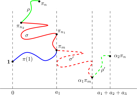
Figure 6.1. The solid SAW lies in $B_{n}(a_{1},a_{2},a_{3})$. We map the red path connecting $\pi_{n_{2}}$ to $\pi_{m}$, and also the third sub-SAW of $\pi$, thereby obtaining a SAW in $B_{n}(a_{1}+a_{2}+a_{3})$. After translation, the paths are dashed.

The new SAW $\pi^{\prime}$ is constructed in the following way, as illustrated in Figure 6.1. Suppose first that $k\geq 3$.

• Let $m=\min\{k:h(\pi_{k})=S_{1}\}$, and let $\pi(1)$ be the sub-SAW from $\pi_{0}={\bf 1}$ to the vertex $\pi_{m}$.

• Let $\sigma:=(\pi_{m},\dots,\pi_{n_{2}})$ and $\rho=(\pi_{n_{2}},\dots,\pi_{n})$ be the two sub-SAWs of $\pi$ with the given endvertices. We find $\alpha_{1}\in{\mathcal{H}}$ such that $\alpha_{1}\pi_{n_{2}}=\pi_{m}$. (This uses the transitive action of ${\mathcal{H}}$.) The concatenation of the two SAWs $\pi(1)$ and $\alpha_{1}\sigma$ (reversed) is a SAW, denoted $\pi(2)$, from ${\bf 1}$ to $\alpha_{1}\pi_{m}$. In concluding that $\pi(2)$ is a SAW, we have made use of Definition 3.1(b). Note that $h(\alpha_{1}\pi_{m})=a_{1}+a_{2}$.

• We next find $\alpha_{2}\in{\mathcal{H}}$ such that $\alpha_{2}(\pi_{n_{2}})=\alpha_{1}(\pi_{m})$. The concatenation of the two SAWs $\pi(2)$ and $\alpha_{2}\rho$ is a SAW, denoted $\pi^{\prime}$, from ${\bf 1}$ to $\alpha_{2}\pi_{n}$. Note that $S_{1}(\pi^{\prime})=a_{1}+a_{2}+a_{3}$.

The ensuing $\pi^{\prime}$ satisfies $\pi^{\prime}\in B_{n}(a_{1}+a_{2}+a_{3},a_{4},\dots,a_{k})$. Note that $\pi$ is not generally reconstructible from knowledge of $\pi^{\prime}$.

Suppose now that $k=2$. At Step 2 above, we have that $h(\pi_{n})=S_{1}-S_{2}$, so that $n_{2}=n$ and $\pi^{\prime}\in B_{n}(a_{1}+a_{2})$.

We consider next the multiplicities associated with the map $\pi\mapsto\pi^{\prime}$: (i) for given $\pi$, how many possible choices of $\pi^{\prime}$ exist, and (ii) for given $\pi^{\prime}$, how many pre-images are there? There are two stages to be considered, arising in Steps 2 and 3 above. We begin at Step 2.

We assume $k\geq 3$ (the case $k=2$ is similar). In the above construction, we map $\pi$ to $\pi^{\prime}$, and we write $\pi=(\pi(1),\sigma,\rho)$ and $\pi^{\prime}=(\pi(1),\sigma^{\prime},\rho^{\prime})$ as in Figure 6.1, where $\sigma^{\prime}=\alpha_{1}\sigma$ and $\rho^{\prime}=\alpha_{2}\rho$. Note that, for given $(a_{i})$, $\pi$ and $\pi^{\prime}$ have unique representations in this form. The representation of $\pi$ is given as above; for given such $\pi^{\prime}$, $\pi(2)$ is the shortest sub-SAW from ${\bf 1}$ to a vertex with height $a_{1}$, $\rho^{\prime}$ is the shortest sub-SAW from a vertex with height $a_{1}+a_{2}$ to the final endvertex of $\pi^{\prime}$, and $\sigma^{\prime}$ is the remaining SAW. We fix $\pi(1)$ for the moment, and consider the relationship between $\sigma^{\prime}$ and $\sigma$. As usual, $a$ denotes the final endvertex of $\pi(1)$.

Let $a\in V$, $s\geq 1$, and let $\Sigma(a,s)$ be the set of SAWs $\sigma=(\sigma_{0},\sigma_{1},\dots,\sigma_{t})$ with $\sigma_{0}=a$ and satisfying

$$h(\sigma_{t})=h(a)-s,\qquad h(a)-s\leq h(\sigma_{l})\leq h(a)\quad\text{for}\quad 1\leq l\leq t.$$

Write $\Sigma:=\Sigma(a,a_{2})$. The SAW $\sigma$ ranges over the subset $\overline{\Sigma}\subseteq\Sigma$ comprising all $\sigma_{1}\in\Sigma$ that do not intersect $\pi(1)$ (other than at $a$). By Lemma 6.4, the image $\sigma^{\prime}$ lies in the set $I:=\bigcup\{{\mathcal{H}}_{b_{1},a}\sigma_{1}:\sigma_{1}\in\Sigma\}$, where $b_{1}$ denotes the endvertex of $\sigma_{1}$ other than $a$. Now, $\Sigma$ may be partitioned as ${\mathcal{P}}=\{{\mathcal{H}}_{a,a}\sigma:\sigma\in\Sigma\}$, and similarly $I$ may be partitioned as ${\mathcal{P}}^{\prime}=\{{\mathcal{H}}_{a,a}\sigma^{\prime}:\sigma^{\prime}\in I\}$. By Lemma 6.4, there is a one-to-one correspondence between ${\mathcal{P}}$ and ${\mathcal{P}}^{\prime}$, and any corresponding pair $(P_{1},P_{2})\in{\mathcal{P}}\times{\mathcal{P}}^{\prime}$ of sets satisfies $|P_{1}|=|P_{2}|$. It follows that

(6.8) $$|\overline{\Sigma}|\leq|\Sigma|=|I|.$$

A simpler argument is valid for the pair $(\rho,\rho^{\prime})$ arising at Step 3. Write $c$ for the endvertex of $\sigma^{\prime}$ other than $a$. Then $\rho$ ranges over a subset $\overline{B}\subseteq B_{n-m}^{b}(a_{3},\dots,a_{k})$ where $m$ is the length of $\pi(1)\cup\sigma$, and its image $\rho^{\prime}$ lies in ${\mathcal{H}}_{b,c}B_{n-m}^{b}(a_{3},\dots,a_{k})$. (As earlier, $b$ denotes the initial vertex of $\rho$.) Hence,

(6.9) $$|\overline{B}|\leq\bigl{|}B_{n-m}^{b}(a_{3},\dots,a_{k})\bigr{|}=\bigl{|}B_{n-m}^{c}(a_{3},\dots,a_{k})\bigr{|},$$

since, by transitivity, the last two sets are in one-to-one correspondence.

The set $B_{n}(a_{1},a_{2},\dots,a_{k})$ is the union of all such $(\pi(1),\sigma,\rho)$. Inequality (6.6) follows by (6.8)–(6.9). Lemma 6.5 is proved. ∎

Write $\sum_{a}^{(k,T)}$ for the summation over all finite integer sequences $a_{1}>\dots>a_{k}>0$ with given length $k$ and sum $T$. By iteration of (6.6),

(6.10) $$c_{n} \leq\sum_{T=1}^{dn}\sum_{k=1}^{n}\sum_{a}^{(k,T)}\bigl{|}B_{n}(a_{1},\dots,a_{k})\bigr{|}$$

$$\leq\sum_{T=1}^{dn}\sum_{k=1}^{n}\sum_{a}^{(k,T)}|B_{n}(a_{1}+a_{2}+\dots+a_{k})|.$$

By (6.2), there exists an absolute constant $A$ such that

(6.11) $$c_{n} \leq\sum_{T=1}^{dn}\sum_{k=1}^{n}\sum_{a}^{(k,T)}b_{n}\leq e^{A\sqrt{dn}}b_{n},$$

as required for Proposition 6.2. ∎

Proposition 6.6.

There exists an absolute constant $B$ such that $\sigma_{n}\leq e^{B\sqrt{dn}}b_{n+1}$ for $n\geq 1$.

Proof.

Let $\pi=(\pi_{0},\pi_{1},\dots,\pi_{n})\in\Sigma_{n}$. Let $H=\min_{0\leq i\leq n}h(\pi_{i})$ and $m=\max\{i:h(\pi_{i})=H\}$. For each such $\pi$, we send one unit of mass from $\pi_{0}$ to $\pi_{m}$, so that the total mass leaving each $v\in V$ is $\sigma_{n}$. By the mass transport principle (see [27, Eqn (8.4)]), the total mass arriving at each $v\in V$ is also $\sigma_{n}$.

Each $\pi\in\Sigma_{n}$, seen from the vertex $\pi_{m}$, is the union of two SAWs $\pi(1)=(\pi_{m},\pi_{m-1},\dots,\pi_{0})$ and $\pi(2)=(\pi_{m},\pi_{m+1},\dots,\pi_{n})$. These two SAWs are vertex-disjoint except at $\pi_{m}$, and $\pi(2)$ is a half-space SAW. We pick $w\in\partial\pi_{m}$ such that $h(w)<h(\pi_{m})$, and extend $\pi(1)$ by adding $w$ at the start, thus obtaining a $(m+1)$-step half-space SAW. Therefore,

$$\sigma_{n}\leq\sum_{m=0}^{n}c_{m+1}c_{n-m}.$$

By Proposition 6.2,

$$\sigma_{n}\leq\sum_{m=0}^{n}U_{m+1}U_{n-m},$$

where $U_{k}=e^{A\sqrt{dk}}b_{k}$. Therefore,

$$\sigma_{n} \leq\sum_{m=0}^{n}\exp\Bigl{(}A\sqrt{d(m+1)}+A\sqrt{d(n-m)}\Bigr{)}b_{m+1}b_{n-m}$$

$$\leq e^{A\sqrt{2d(n+1)}}b_{n+1},$$

by (4.3) and the fact that $\sqrt{x}+\sqrt{y}\leq\sqrt{2x+2y}$. The claim follows. ∎

It is trivial that $b_{n}\leq\sigma_{n}$, whence $\beta\leq\mu$. The reverse inequality follows by Proposition 6.6, and Theorem 4.3 is proved in the transitive case.

7. Theorem 4.3: the quasi-transitive case

We present the further steps needed to prove Theorem 4.3 when the unimodular graph height function $(h,{\mathcal{H}})$ is such that ${\mathcal{H}}$ acts only quasi-transitively on $G$. Proposition 6.2 is replaced by the following. Recall the maximum vertex-degree $\delta_{G}$, and the integer $r$ given before Proposition 3.2.

Proposition 7.1.

There exists $A=A(d,r,\delta_{G})$, that is non-decreasing in $d$, $r$, and $\delta_{G}$, such that $c_{n}(v)\leq e^{A\sqrt{n}}\beta^{n}$ for $n\geq 1$ and $v\in V$.

Proof.

We follow the proof of Proposition 6.2, with the following differences. Let $o_{1},o_{2},\dots,o_{M}$ be representatives of the equivalence classes of ${\mathcal{H}}$. By the definition of $r$, we may choose such $o_{i}$ satisfying $d_{G}(o_{i},o_{j})\leq r$ for all $i,j$. A vertex $v\in V$ is said to have type $o_{i}$ if $v\in{\mathcal{H}}o_{i}$. Lemmas 6.3 and 6.4 are replaced by the following.

Lemma 7.2.

Let $\sigma$ be a SAW with initial (respectively, final) vertex $a$ (respectively, $b$), and assume $a$ has type $o_{a}$ and $b$ has type $o_{b}$. There exist constants $\xi_{1},\xi_{2},\dots,\xi_{M}>0$, depending on $G$ and ${\mathcal{H}}$ only, such that, for $v,w\in V$ with respective types $o_{a}$ and $o_{b}$,

(7.1) $$\frac{1}{\xi_{a}}|{\mathcal{H}}_{a,v}\sigma|=\frac{1}{\xi_{b}}|{\mathcal{H}}_{b,w}\sigma|.$$

Furthermore,

(7.2) $$\xi:=\max\bigl{\{}\xi_{i}/\xi_{j}:i,j=1,2,\dots,M\bigr{\}}$$

satisfies $\xi\leq|S_{2r}({\bf 1})|$, and hence

(7.3) $$\xi\leq\frac{\delta_{G}^{2r+1}-1}{\delta_{G}-1}.$$

Proof.

Equation (7.1) follows by adapting the proof of Proposition 6.2 and appealing to [27, Cor. 8.11]. By [27, Thm 8.10],

$$\frac{\xi_{i}}{\xi_{j}} =\frac{|\textrm{Stab}_{o_{i}}o_{j}|}{|\textrm{Stab}_{o_{j}}o_{i}|}\leq|\textrm{Stab}_{o_{i}}o_{j}|$$

$$\leq|S_{r}(o_{i})|\leq|S_{2r}({\bf 1})|,$$

by the definition of $r=r(h,{\mathcal{H}})$. ∎

Lemma 7.3.

Let $a\in V$, $t\geq 1$, and let $\sigma=(\sigma_{0},\sigma_{1},\dots,\sigma_{t})$ be a SAW starting at $\sigma_{0}=a$. Let $b=\sigma_{t}$ and let $b^{\prime}\in V$ have the same type as $b$. Fix $\sigma^{\prime}\in{\mathcal{H}}_{b,b^{\prime}}\sigma$. Consider the bipartite graph $B$ with vertex-sets $R:={\mathcal{H}}_{a,a}\sigma$ (coloured red) and $Y:={\mathcal{H}}_{b^{\prime},b^{\prime}}\sigma^{\prime}$ (coloured yellow), and an edge between $\sigma_{1}\in R$ and $\sigma_{1}^{\prime}\in Y$ if and only if $\sigma_{1}^{\prime}\in{\mathcal{H}}_{b_{1},b^{\prime}}\sigma_{1}$ where $b_{1}$ is the endvertex of $\sigma_{1}$ other than $a$. The graph $B$ is complete bipartite, and $\xi^{-1}|Y|\leq|R|\leq\xi|Y|$ where $\xi$ is given by (7.2).

Proof.

That $B$ is complete bipartite follows as in the proof of Lemma 6.4. The final inequality holds similarly, but using (7.1) in place of (6.3). ∎

Let $\pi\in B_{n}^{v}(a_{1},a_{2},\dots,a_{k})$. We shall perform surgery on $\pi$ to obtain a SAW $\pi^{\prime}$ satisfying

(7.4) $$\pi^{\prime}\in\begin{cases}B_{n+\theta}^{v}(a_{1}+a_{2}+a_{3}+\delta,a_{4},\dots,a_{k})&\text{if }k\geq 3,\\ B_{n+\theta}^{v}(a_{1}+a_{2}+\delta)&\text{if }k=2,\end{cases}$$

for some $\theta=\theta(\pi)$ and $\delta=\delta(\pi)$ satisfying $0\leq\theta\leq 2r$ and $\delta\geq 0$.

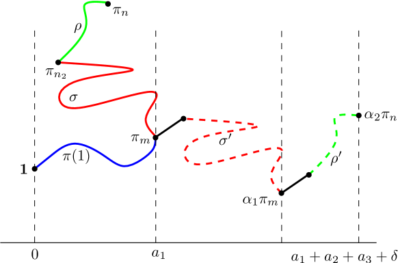
Figure 7.1. In the non-transitive case, further SAWs are introduced in order to make the required connections. These extra connections are drawn in black, and have lengths no greater than $r$.

The SAW $\pi^{\prime}$ is constructed as in Steps 1–3 of the previous proof, but with a significant extra feature. In the construction of $\pi^{\prime}$ in Section 6, the two sub-SAWs $\sigma$ and $\rho$ are mapped to new SAWs with the given starting vertices. This cannot generally be done in the non-transitive setting, since the target starting vertices may not have the appropriate types.

Steps 2 and 3 of the preceding proof are thus replaced as follows (as illustrated in Figure 7.1). The SAWs $\nu(\cdot,\cdot)$ of the following are as given after (3.2).

• Let $\sigma:=(\pi_{m},\dots,\pi_{n_{2}})$ and $\rho=(\pi_{n_{2}},\dots,\pi_{n})$ be the two sub-SAWs of $\pi$ with the given endvertices. The type of $\pi_{m}$ (respectively, $\pi_{n_{2}}$) is denoted $i$ (respectively, $j$). In particular, $\pi_{m}=\gamma(o_{i})$ for some $\gamma\in{\mathcal{H}}$. We map the SAW $\nu(o_{i},v_{j})$, given after (3.2), under $\gamma$ to obtain a SAW denoted $\nu(\pi_{m},\alpha_{1}\pi_{n_{2}})$, where $\alpha_{1}\in{\mathcal{H}}$ is such that $\alpha_{1}(\pi_{n_{2}})=\gamma(v_{j})$. Note that $\nu(\pi_{m},\alpha_{1}\pi_{n_{2}})$ is the single point $\{\pi_{m}\}$ if $i=j$, and $\alpha_{1}(\pi_{n_{2}})=\pi_{m}$ in this case.

  The union of the three SAWs $\pi(1)$, $\nu(\pi_{m},\alpha_{1}\pi_{n_{2}})$, and $\sigma^{\prime}:=\alpha_{1}\sigma$ (reversed) is a SAW, denoted $\pi(2)$, from $v$ to $\alpha_{1}\pi_{m}$. Note that $a_{1}+a_{2}\leq h(\alpha_{1}\pi_{m})\leq a_{1}+a_{2}+r$.

• We next perform a similar construction to connect $\alpha_{1}\pi_{m}$ to an image of the first vertex $\pi_{n_{2}}$ of $\rho$. These two vertices have types $i$ and $j$, as before, and thus we insert the SAW $\nu(\alpha_{1}\pi_{m},\alpha_{2}\pi_{n_{2}}):=\alpha_{1}\gamma\nu(o_{i},v_{j})$, where $\alpha_{2}\in{\mathcal{H}}$ is such that $\alpha_{2}(\pi_{n_{2}})=\alpha_{1}\gamma(v_{j})$. The union of the three SAWs $\pi(2)$, $\nu(\alpha_{1}\pi_{m},\alpha_{2}\pi_{n_{2}})$, and $\rho^{\prime}:=\alpha_{2}\rho$, is a SAW, denoted $\pi^{\prime}$, from ${\bf 1}$ to $\alpha_{2}\pi_{n}$.

The resulting SAW satisfies $\pi^{\prime}\in B_{n+\theta}^{v}(a_{1}+a_{2}+a_{3}+\delta,a_{4},\dots,a_{k})$ for some $0\leq\theta\leq 2r$ and $\delta\geq 0$. In this non-transitive scenario, there are two reasons for which $\pi$ is not generally reconstructible from knowledge of $\pi^{\prime}$: (i) we need to identify the intermediate SAWs $\nu(\cdot)$, and (ii) the maps $\sigma\mapsto\sigma^{\prime}$ and $\rho\mapsto\rho^{\prime}$ are not bijections. Since the intermediate SAWs have lengths no greater than $r$, issue (i) contributes at worst a factor $(r+1)^{2}$ when $k\geq 3$ (and a factor $(r+1)$ when $k=2$). Issue (ii) is controlled as in the previous proof, using Lemma 7.3 in place of Lemma 7.2, thus introducing a factor $\xi^{k}$.

Equation (6.10) is replaced in the quasi-transitive context by

$$c_{n}(v) \leq\sum_{T=1}^{dn}\sum_{k=1}^{n}\sum_{a}^{(k,T)}\bigl{|}B_{n}^{v}(a_{1},\dots,a_{k})\bigr{|}$$

$$\leq\sum_{T=1}^{dn}\sum_{k=1}^{n}\sum_{a}^{(k,T)}\xi^{k}(r+1)^{k}\sum_{s=0}^{kr}b_{n+s}(v).$$

As in (6.11), by (4.7), (7.3), and that fact that $\beta\leq\delta_{G}$, there exists a constant $A=A(d,r,\delta_{G})$ with the required properties such that

$$c_{n}(v) \leq\sum_{T=1}^{dn}\sum_{k=1}^{n}\sum_{a}^{(k,T)}\xi^{k}(r+1)^{k}(kr+1)\beta^{n+kr+r}$$

$$\leq\sum_{T=1}^{dn}\sum_{k=1}^{n}\sum_{a}^{(k,T)}\beta^{n+r}\{\beta^{r}\xi(r+1)\}^{\sqrt{2dn}}\bigl{(}r\sqrt{2dn}+1\bigr{)}$$

$$\leq e^{A\sqrt{n}}\beta^{n},$$

as required. ∎

Proposition 7.4.

There exists $B=B(d,r,\delta_{G})>0$, that is non-decreasing in $d$, $r$, and $\delta_{G}$, such that $\sigma_{n}(v)\leq e^{B\sqrt{n}}\beta^{n}$ for $n\geq 1$ and $v\in V$.

Proof.

We adapt the proof of Proposition 6.6 to the quasi-transitive setting. By the mass transport principle, as there,

$$\sum_{i}\frac{1}{\xi_{i}}\sigma_{n}(o_{i})=\sum_{j}\frac{1}{\xi_{j}}I(o_{j}),$$

where $I(v)$ denotes the total mass entering the vertex $v$. Therefore,

$$\sigma_{n}(v)\leq\xi M\sum_{m=0}^{n}U_{m+1}U_{n-m},$$

where $U_{k}=e^{A\sqrt{k}}\beta^{k}$ and $M=M({\mathcal{H}})$ is the number of equivalence classes of ${\mathcal{H}}$. The proof is completed as before. ∎

References

- [1] L. Babai, Vertex-transitive graphs and vertex-transitive maps, J. Graph Th. 15 (1991), 587–627.
- [2] R. Bauerschmidt, H. Duminil-Copin, J. Goodman, and G. Slade, Lectures on self-avoiding walks, Probability and Statistical Physics in Two and More Dimensions (D. Ellwood, C. M. Newman, V. Sidoravicius, and W. Werner, eds.), Clay Mathematics Institute Proceedings, vol. 15, CMI/AMS publication, 2012, pp. 395–476.
- [3] I. Benjamini, Euclidean vs graph metric, Erdős Centennial (L. Lovász, I. Ruzsa, and V. T. Sós, eds.), Springer, 2013, pp. 35–57.
- [4] I. Benjamini, A. Nachmias, and Y. Peres, Is the critical percolation probability local?, Probab. Th. Rel. Fields 149 (2011), 261–269.
- [5] I. Benjamini and O. Schramm, Recurrence of distributional limits of finite planar graphs, Electron. J. Probab. 6 (2001), Article 23.
- [6] T. Bodineau, Slab percolation for the Ising model, Probab. Th. Rel. Fields 132 (2005), 83–118.
- [7] S. R. Broadbent and J. M. Hammersley, Percolation processes. I. Crystals and mazes, Proc. Camb. Phil. Soc. 53 (1957), 629–641.
- [8] D. Cimasoni and H. Duminil-Copin, The critical temperature for the Ising model on planar doubly periodic graphs, Electron. J. Probab. 18 (2013), Article 44.
- [9] R. Diestel and I. Leader, A conjecture concerning a limit of non-Cayley graphs, J. Alg. Combin. 14 (2001), 17–25.
- [10] R. L. Dobrushin, Prescribing a system of random variables by the help of conditional distributions, Theory Probab. and its Appl. 15 (1970), 469–497.
- [11] R. L. Dobrushin and S. B. Shlosman, Constructive criterion for the uniqueness of a Gibbs field, Statistical Mechanics and Dynamical Systems (J. Fritz, A. Jaffe, and D. Szasz, eds.), Birkhäuser, Boston, 1985, pp. 347–370.
- [12] M. J. Dunwoody, An inaccessible graph, Random Walks, Boundaries and Spectra, Progr. Probab., vol. 64, Birkhäuser/Springer Basel AG, Basel, 2011, pp. 1–14.
- [13] A. Eskin, D. Fisher, and K. Whyte, Quasi-isometries and rigidity of solvable groups, Pure Appl. Math. Quart. 3 (2007), 927–947.
- [14] P. Flory, Principles of Polymer Chemistry, Cornell University Press, 1953.
- [15] G. R. Grimmett and Z. Li, Self-avoiding walks and the Fisher transformation, Electron. J. Combin. 20 (2013), Paper P47.
- [16] by same author, Strict inequalities for connective constants of regular graphs, SIAM J. Disc. Math. 28 (2014), 1306–1333.
- [17] by same author, Bounds on the connective constants of regular graphs, Combinatorica 35 (2015), 279–294.
- [18] by same author, Connective constants and height functions for Cayley graphs, Trans. Amer. Math. Soc. 369 (2017), 5961–5980.
- [19] by same author, Self-avoiding walks and amenability, Elect. J. Combin. 24 (2017), paper P4.38, 24 pp.
- [20] by same author, Self-avoiding walks and connective constants, (2017), http://arxiv.org/abs/1704.05884.
- [21] G. R. Grimmett and J. M. Marstrand, The supercritical phase of percolation is well behaved, Proc. Roy. Soc. London Ser. A 430 (1990), 439–457.
- [22] J. M. Hammersley, Percolation processes II. The connective constant, Proc. Camb. Phil. Soc. 53 (1957), 642–645.
- [23] J. M. Hammersley and W. Morton, Poor man’s Monte Carlo, J. Roy. Statist. Soc. B 16 (1954), 23–38.
- [24] J. M. Hammersley and D. J. A. Welsh, Further results on the rate of convergence to the connective constant of the hypercubical lattice, Quart. J. Math. Oxford 13 (1962), 108–110.
- [25] G. H. Hardy and S. Ramanujan, Asymptotic formulae for the distribution of integers of various types, Proc. Lond. Math. Soc. 16 (1917), 112–132.
- [26] Z. Li, Critical temperature of periodic Ising models, Commun. Math. Phys. 315 (2012), 337–381.
- [27] R. Lyons and Y. Peres, Probability on Trees and Networks, Cambridge University Press, Cambridge, 2016, http://mypage.iu.edu/~rdlyons/.
- [28] N. Madras and G. Slade, Self-Avoiding Walks, Birkhäuser, Boston, 1993.
- [29] S. Martineau and V. Tassion, Locality of percolation for abelian Cayley graphs, Ann. Probab. 45 (2017), 1247–1277.
- [30] V. I. Trofimov, Automorphism groups of graphs as topological groups, Math. Notes 38 (1985), 717–720.
- [31] D. Weitz, Combinatorial criteria for uniqueness of Gibbs measures, Rand. Struct. Alg. 2005 (27), 445–475.