The impact of startup costs and the grid operator on the power price equilibrium

Abstract

In this paper we propose a quadratic programming model that can be used for calculating the term structure of electricity prices while explicitly modeling startup costs of power plants. In contrast to other approaches presented in the literature, we incorporate the startup costs in a mathematically rigorous manner without relying on ad hoc heuristics. Moreover, we propose a tractable approach for estimating the startup costs of power plants based on their historical production. Through numerical simulations applied to the entire UK power grid, we demonstrate that the inclusion of startup costs is necessary for the modeling of electricity prices in realistic power systems. Numerical results show that startup costs make electricity prices very spiky. In the second part of the paper, we extend the initial model by including the grid operator who is responsible for managing the grid. Numerical simulations demonstrate that robust decision making of the grid operator can significantly decrease the number and severity of spikes in the electricity price and improve the reliability of the power grid.

1 Introduction

More than two decades ago, electricity markets started the transition from a regulated market with a single utility company to a fully competitive market. This introduced a need for a development of financial models that would help us to understand the behavior of electricity prices and manage the risk. High uncertainty in the electricity demand and fuel prices requires robust models, so that low electricity prices and a reliable delivery of electricity can be achieved.

Electricity markets are changing extremely quickly, often faster than any other financial markets. High pressure on decarbonization has led to new market design and policies. New, intermittent, renewable sources are connected to the electricity grid almost on a daily basis. Smart grids, together with the battery storage and demand response, are making their way into market. All these inventions have an impact on the electricity price and its behavior. The pace of new inventions makes the risk management and decision making in electricity markets very challenging.

In the literature, there exist three approaches to the modeling of electricity prices. Traditionally, electricity prices have been modeled by so called non-structural approaches. These approaches attempt to model electricity prices directly without explicitly considering the fundamental factors that drive such behavior. [17] investigated the statistical properties of the electricity prices at the Nordic Power Exchange. The suitability of one and multi-factor Ornstein-Uhlenbeck processes for modeling the spot as well as the log spot price was examined. As pointed out in this work, none of these models are able to capture the spikes in the electricity price. Thus, various other models that combine the Ornstein-Uhlenbeck process with a pure jump-process (see [14] for example) or more general Levy process (see [19] and [11] for example) were proposed. A one-factor model in [7] and multi-factor term-structure model in [6] are the first that produce prices that are consistent with observable forward prices. While non-structural models are widely used for the short-term risk management as well as electricity derivatives pricing purposes in practice, they do not cater well for longer-term modeling purposes, where the impact of new inventions must be included. They must be frequently recalibrated to reflect the changes in the markets.

Structural approaches for modeling electricity prices capture some of the fundamental factors of the electricity market. The supply and demand stack was first used to model electricity prices in [1]. This idea was extended by [16] and by [5], where an exponential supply and demand stack was modeled as a function of the underlying fuels such as natural gas and coal.

The third, game theoretic, approach models the electricity market even more closely. The disastrous events that happened in California in 2001 confirmed that some physical properties of power plants such as ramp-up and ramp-down constants, and market design together with the transmission lines play a vital role in the behavior of electricity prices. The first game theoretic model for modeling the electricity prices was proposed in [2], where a unique relation between a forward and a spot price is given in a two-stage market with one producer and one consumer, who each want to maximize their mean-variance objective function. This model was extended to a multistage setting in [4] and [3], and to any convex risk measure in [8]. [21] further extended the work of [3] to a setting with more than one producer and consumer, who optimize their mean-variance objective functions. In contrast to other game theoretic models, capacity and ramp-up and ramp-down constraints of power plants are included. By modeling the profit of power plants as a difference between the power price and fuel costs together with emissions obligations, this work also incorporates ideas from the structural approach. As in [6] and [7], the model is consistent with observable fuel and emission prices. [20] applied this model to calculate the electricity prices in the UK by taking into account the entire power grid consisting of a few hundred power plants. Numerical simulations show that this model has a tendency to underestimate spot prices during the peak hours and to overestimate them during the off-peak hours. It is argued that this may occur because startup costs are not included in the model.

In this paper, we extend the model presented in [20] and include the startup costs. Various methodologies have already been proposed on how to include the startup costs (see [18], [12] and [23] for example). Most of them rely on a price uplift approach, where first the power price without startup costs is calculated. This price is then uplifted to reflect the startup costs. In our model, the startup costs are included in a mathematically rigorous fashion without relying on the uplift heuristic.

We show that startup costs are responsible for introducing many spikes in spot electricity prices. To reduce the number of spikes, we include the grid operator, who is responsible for managing the grid and for a reliable delivery of electricity, by enhancing our model in the second part of the paper.

This paper is organized as follows: In Section 2 we give a detailed mathematical description of the model, and in Section 3 we present the numerical results. Numerical results motivate us to introduce the grid operator in Section 4. We conclude the paper in Section 5.

2 Problem description

In this section we provide a detailed description of a model that we use for the purpose of modeling the term structure of electricity prices. The model belongs to a class of game theoretic equilibrium models. Market participants are divided into consumers and producers. A set of consumers is denoted by $C$ and has cardinality $0<\left|C\right|<\infty$. Similarly, a set of producers is denoted by $P$ and has cardinality $0<\left|P\right|<\infty$. Each producer owns a portfolio of power plants that can have different characteristics such as capacity, startup costs, ramp-up and ramp-down constraints, efficiency, and fuel type. The set of all fuel types is denoted by $L$. Sets $R^{p,l}$ denote all power plants owned by producer $p\in P$ that run on fuel $l\in L$. A set $R^{p,l}$ may be empty since each producer typically does not own all possible types of power plants. Moreover, this allows us to include non physical traders such as banks or speculators, who do not own any electricity generation facilities and are without a physical demand for electricity, as producers $p\in P$ with $R^{p,l}=\left\{\right\}$ for all $l\in L$.

As we will see in Section 2.4, it is useful to introduce another player named the hypothetical market agent besides producers and consumers. The hypothetical market agent plays the role of the electricity market and ensures that the term structure of the electricity price is such that the market clearing condition is satisfied for all electricity forward contracts.

We are interested in delivery times $T_{j}$, $j\in J=\left\{1,...,T^{\prime}\right\}$, where power for each delivery time $T_{j}$ can be traded through numerous forward contracts at times $t_{i}$, $i\in I_{j}$. The electricity price at time $t_{i}$ for delivery at time $T_{j}$ is denoted by $\Pi\left(t_{i},T_{j}\right)$. Since contracts with trading time later than delivery time do not exist, we require $t_{\max\left\{I_{j}\right\}}=T_{j}$ for all $j\in J$. The number of all forward contracts, i.e. $\sum_{j\in J}\left|I_{j}\right|$, is denoted by $N$. Uncertainty is modeled by a filtered probability space $\left(\Omega,\mathcal{F},\mathbb{F}=\left\{\mathcal{F}_{t},t\in I\right\},\mathbb{P}\right)$, where $I=\cup_{j\in J}I_{j}$. The $\sigma$-algebra $\mathcal{F}_{t}$ represents information available at time $t$.

The exogenous variables that appear in our model are (a) aggregate power demand $D\left(T_{j}\right)$ for each delivery period $j\in J$, (b) prices of fuel forward contracts $G_{l}\left(t_{i},T_{j}\right)$ for each fuel $l\in L$, delivery period $j\in J$, and trading period $i\in I_{j}$, and (c) prices of emissions forward contracts $G_{em}\left(t_{i},T_{j}\right)$, $j\in J$, $i\in I_{j}$. Electricity prices and all exogenous variables are assumed to be adapted to the filtration $\left\{\mathcal{F}_{t}\right\}_{t\in I}$ and have finite second moments.

Let $v_{k}\in\mathbb{R}^{n_{k}}$, $n_{k}\in\mathbb{N}$, $k\in K$, and $K=\left\{1,...,\left|K\right|\right\}$ be given vectors. For convenience, we define a vector concatenation operator as

$$\left|\right|_{k\in K}v_{k}=\left[v_{1}^{\top},...,v_{\left|K\right|}^{\top}\right]^{\top}.$$

2.1 Producers

Each producer $p\in P$ participates in the electricity, fuel, and emission markets. Forward as well as spot contracts are available on all markets. Electricity prices, fuel prices, and emission prices are denoted by $\Pi\left(t_{i},T_{j}\right)$, $G_{l}\left(t_{i},T_{j}\right)$ where $l\in L$, and $G_{em}\left(t_{i},T_{j}\right)$, respectively.

A producer may participate in the market by buying and selling forward and spot contracts. The number of electricity forward contracts that producer $p\in P$ buys at trading time $t_{i}$, $i\in I_{j}$ for delivery at time $T_{j}$, $j\in J$ is denoted by $V_{p}\left(t_{i},T_{j}\right)$. Similarly, the number of fuel and emission forward contracts that producer $p\in P$ buys at trading time $t_{i}$, $i\in I_{j}$ for delivery at time $T_{j}$, $j\in J$ is denoted by $F_{p,l}\left(t_{i},T_{j}\right)$, $l\in L$ and $O_{p}\left(t_{i},T_{j}\right)$, respectively. Producers own a generally non-empty portfolio of power plants. The actual production of electricity from power plant $r\in R^{p,l}$ at delivery time $T_{j}$, $j\in J$ is denoted by $\widehat{W}_{p,l,r}\left(T_{j}\right)$.

2.1.1 Production variables

In this section we investigate the production of power plants more closely. Each power plant $r\in R^{p,l}$, $p\in P$, $l\in L$ has a maximum export limit and minimum stable limit denoted by $\overline{W}_{max}^{p,l,r}\left(T_{j}\right)$ and $\overline{W}_{min}^{p,l,r}\left(T_{j}\right)$, respectively. The maximum export limit defines the maximum production capacity of a power plant and the minimum stable limit defines the minimum production that a power plant is able to maintain for a longer period of time. We allow each of the parameters to be time dependent to account for the maintenance of power plants.

Stable production of each power plant must satisfy

(1) $$\widehat{W}_{p,l,r}\left(T_{j}\right)\in\left\{0\right\}\cup\left[\overline{W}_{min}^{p,l,r}\left(T_{j}\right),\overline{W}_{max}^{p,l,r}\left(T_{j}\right)\right]$$

for each $j\in J$. It is allowed for a power plant to have production $\widehat{W}_{p,l,r}\left(T_{j}\right)\in\left(0,\overline{W}_{min}^{p,l,r}\left(T_{j}\right)\right)$ for a very short period of time (i.e. during a ramp-up and ramp-down phase). To formulate these constraints in an optimization framework, we introduce new decision variables $W_{p,l,r}^{\left(k\right)}\left(T_{j}\right)$, $k\in\left\{1,...,6\right\}$ with the following meaning:

• $W_{p,l,r}^{\left(1\right)}\left(T_{j}\right)$, $j\in J$ is a continuous variable that is $1$ if the power plant is fully ramped up at time $T_{j}$ and $0$ if the power plant is not producing at all at time $T_{j}$. If $W_{p,l,r}^{\left(1\right)}\left(T_{j}\right)\in\left(0,1\right)$ then the power plant is in the ramp-up or ramp-down phase. In an optimization framework, $W_{p,l,r}^{\left(1\right)}\left(T_{j}\right)$ is defined as

  (2) $$W_{p,l,r}^{\left(1\right)}\left(T_{j}\right)\in\left[0,1\right].$$

• $W_{p,l,r}^{\left(2\right)}\left(T_{j}\right)$, $j\in J$ is a binary variable that is $1$ if the power plant is fully ramped up at time $T_{j}$ and $0$ otherwise. In an optimization framework, $W_{p,l,r}^{\left(2\right)}\left(T_{j}\right)$ is defined as

  (3) $$\begin{array}[]{c}W_{p,l,r}^{\left(2\right)}\left(T_{j}\right)\leq W_{p,l,r}^{\left(1\right)}\left(T_{j}\right)\\ \\ W_{p,l,r}^{\left(2\right)}\left(T_{j}\right)\in\left[0,1\right]\end{array}$$

  and

  (4) $$W_{p,l,r}^{\left(2\right)}\left(T_{j}\right)\in\mathbb{Z}.$$

• $W_{p,l,r}^{\left(3\right)}\left(T_{j}\right)$, $j\in J\backslash\left\{1\right\}$ is a continuous variable that denotes the increase of $W_{p,l,r}^{\left(1\right)}\left(T_{j}\right)$ from time $T_{j-1}$ to time $T_{j}$. In an optimization framework, $W_{p,l,r}^{\left(3\right)}\left(T_{j}\right)$ is defined as

  (5) $$W_{p,l,r}^{\left(3\right)}\left(T_{j}\right)\geq W_{p,l,r}^{\left(1\right)}\left(T_{j}\right)-W_{p,l,r}^{\left(1\right)}\left(T_{j-1}\right)$$

  and

  (6) $$W_{p,l,r}^{\left(3\right)}\left(T_{j}\right)\in\left[0,1\right].$$

• $W_{p,l,r}^{\left(4\right)}\left(T_{j}\right)$, $j\in J\backslash\left\{1\right\}$ is a binary variable that is $1$ if the power plant is in the ramp-up phase and $0$ otherwise. In an optimization framework, $W_{p,l,r}^{\left(4\right)}\left(T_{j}\right)$ is defined as

  (7) $$\begin{array}[]{c}W_{p,l,r}^{\left(4\right)}\left(T_{j}\right)\geq W_{p,l,r}^{\left(1\right)}\left(T_{j}\right)-W_{p,l,r}^{\left(1\right)}\left(T_{j-1}\right)\\ \\ W_{p,l,r}^{\left(4\right)}\left(T_{j}\right)\in\left[0,1\right]\end{array}$$

  and

  (8) $$W_{p,l,r}^{\left(4\right)}\left(T_{j}\right)\in\mathbb{Z}.$$

• $W_{p,l,r}^{\left(5\right)}\left(T_{j}\right)$, $j\in J\backslash\left\{1\right\}$ is a binary variable that is $1$ if the power plant is in the ramp-down phase and $0$ otherwise. In an optimization framework, $W_{p,l,r}^{\left(5\right)}\left(T_{j}\right)$ is defined as

  (9) $$\begin{array}[]{c}W_{p,l,r}^{\left(5\right)}\left(T_{j}\right)\geq W_{p,l,r}^{\left(1\right)}\left(T_{j-1}\right)-W_{p,l,r}^{\left(1\right)}\left(T_{j}\right)\\ \\ W_{p,l,r}^{\left(5\right)}\left(T_{j}\right)\in\left[0,1\right]\end{array}$$

  and

  (10) $$W_{p,l,r}^{\left(5\right)}\left(T_{j}\right)\in\mathbb{Z}.$$

• $W_{p,l,r}^{\left(6\right)}\left(T_{j}\right)$, $j\in J$ is a continuous variable such that

  (11) $$\widehat{W}_{p,l,r}\left(T_{j}\right)=W_{p,l,r}^{\left(1\right)}\left(T_{j}\right)\overline{W}_{min}^{p,l,r}\left(T_{j}\right)+W_{p,l,r}^{\left(6\right)}\left(T_{j}\right)\left(\overline{W}_{max}^{p,l,r}\left(T_{j}\right)-\overline{W}_{min}^{p,l,r}\left(T_{j}\right)\right)$$

  where

  (12) $$W_{p,l,r}^{\left(6\right)}\left(T_{j}\right)\leq W_{p,l,r}^{\left(2\right)}\left(T_{j}\right)$$

  and

  (13) $$W_{p,l,r}^{\left(6\right)}\left(T_{j}\right)\in\left[0,1\right].$$

Variable $W_{p,l,r}^{\left(1\right)}\left(T_{j}\right)$ tells us whether the power plant is running at time $T_{j}$. If the power plant is not running at time $T_{j}$, then by (3) and (12), $W_{p,l,r}^{\left(6\right)}\left(T_{j}\right)=0$ and by (11) also $\widehat{W}_{p,l,r}\left(T_{j}\right)=0$. On the other hand, if the power plant is fully ramped up time $T_{j}$, then $W_{p,l,r}^{\left(1\right)}\left(T_{j}\right)=1$ and $W_{p,l,r}^{\left(6\right)}\left(T_{j}\right)\in\left[0,1\right]$, and thus $\widehat{W}_{p,l,r}\left(T_{j}\right)\in\left[\overline{W}_{min}^{p,l,r}\left(T_{j}\right),\overline{W}_{max}^{p,l,r}\left(T_{j}\right)\right]$.

2.1.2 Maximum ramp-up and maximum ramp-down constraints

Producer $p\in P$ is not able to arbitrarily choose her decision variables because there are some constraints that limit her feasible set. The change in production of each power plant from one delivery period to next is limited by the ramp-up and ramp-down constraints. For each $j\in\left\{1,...,T^{\prime}-1\right\}$, where $T^{\prime}$ denotes the last delivery period, $l\in L$ and $r\in R^{p,l}$ these constraints can be expressed as

(14) $$\triangle\overline{W}_{min}^{p,l,r}\left(T_{j}\right)\leq\widehat{W}_{p,l,r}\left(T_{j+1}\right)-\widehat{W}_{p,l,r}\left(T_{j}\right)\leq\triangle\overline{W}_{max}^{p,l,r}\left(T_{j}\right),$$

where $\triangle\overline{W}_{max}^{p,l,r}$ and $\triangle\overline{W}_{min}^{p,l,r}$ represent maximum rates for ramping up and down, respectively. The ramping rates highly depend on the type of the power plant. Some gas power plants can increase production from zero to the maximum in just a few minutes, while the same action may take days or weeks for a nuclear power plant.

Using (11), we can rewrite Constraint (14) for all $j\in\left\{1,...,T^{\prime}-1\right\}$ as

(15) $$\begin{array}[]{rcl}\overline{W}_{min}^{p,l,r}\left(T_{j}\right)&\leq&W_{p,l,r}^{\left(1\right)}\left(T_{j+1}\right)\overline{W}_{min}^{p,l,r}\left(T_{j+1}\right)+W_{p,l,r}^{\left(6\right)}\left(T_{j+1}\right)\left(\overline{W}_{max}^{p,l,r}\left(T_{j+1}\right)-\overline{W}_{min}^{p,l,r}\left(T_{j+1}\right)\right)\\ \\ &&-W_{p,l,r}^{\left(1\right)}\left(T_{j}\right)\overline{W}_{min}^{p,l,r}\left(T_{j}\right)-W_{p,l,r}^{\left(6\right)}\left(T_{j}\right)\left(\overline{W}_{max}^{p,l,r}\left(T_{j}\right)-\overline{W}_{min}^{p,l,r}\left(T_{j}\right)\right)\\ \\ &\leq&\triangle\overline{W}_{max}^{p,l,r}\left(T_{j}\right).\end{array}$$

Additionally, if the power plant is in a ramp-up phase, then it has to increase production and finish the ramp-up phase as fast as possible. Such a requirement can be enforced as

(16) $$W_{p,l,r}^{\left(1\right)}\left(T_{j+1}\right)\geq\min\left\{W_{p,l,r}^{\left(1\right)}\left(T_{j}\right)+\frac{\triangle\overline{W}_{max}^{p,l,r}\left(T_{j}\right)}{\overline{W}_{min}^{p,l,r}\left(T_{j}\right)},1\right\}$$

where $j\in\left\{1,...,T^{\prime}-1\right\}$. Since this constraint is relevant only during the ramp-up phase, we reformulate it for $j\in\left\{1,...,T^{\prime}-1\right\}$ as

(17) $$W_{p,l,r}^{\left(1\right)}\left(T_{j+1}\right)\geq\min\left\{W_{p,l,r}^{\left(1\right)}\left(T_{j}\right)+\frac{\triangle\overline{W}_{max}^{p,l,r}\left(T_{j}\right)}{\overline{W}_{min}^{p,l,r}\left(T_{j}\right)},1\right\}-M_{1}\left(1-W_{p,l,r}^{\left(4\right)}\left(T_{j}\right)\right),$$

where $M_{1}\geq 1+\frac{\triangle\overline{W}_{max}^{p,l,r}\left(T_{j}\right)}{\overline{W}_{min}^{p,l,r}\left(T_{j}\right)}$. Most of the available optimization solvers are not able to handle constraints that include min or max functions. Thus, we apply a well established approach to handle logical constraints, and introduce a new binary decision variable $W_{p,l,r}^{\left(7\right)}\left(T_{j}\right)$ as

(18) $$W_{p,l,r}^{\left(7\right)}\left(T_{j}\right)\in\left[0,1\right]$$

and

(19) $$W_{p,l,r}^{\left(7\right)}\left(T_{j}\right)\in\mathbb{Z}$$

where $j\in J$, that makes sure that at least one of the following constraints

(20) $$W_{p,l,r}^{\left(1\right)}\left(T_{j+1}\right)\geq W_{p,l,r}^{\left(1\right)}\left(T_{j}\right)+\frac{\triangle\overline{W}_{max}^{p,l,r}\left(T_{j}\right)}{\overline{W}_{min}^{p,l,r}\left(T_{j}\right)}-M_{1}\left(1-W_{p,l,r}^{\left(4\right)}\left(T_{j}\right)\right)-M_{2}W_{p,l,r}^{\left(7\right)}\left(T_{j}\right)$$

and

(21) $$W_{p,l,r}^{\left(1\right)}\left(T_{j+1}\right)\geq 1-M_{1}\left(1-W_{p,l,r}^{\left(4\right)}\left(T_{j}\right)\right)-M_{2}\left(1-W_{p,l,r}^{\left(7\right)}\left(T_{j}\right)\right),$$

where $M_{2}\geq 1$, is enforced.

Similarly, if a power plant is in the ramp-down phase, then it has to decrease production and finish the ramp-down phase as fast as possible. Such requirement can be enforced as

(22) $$W_{p,l,r}^{\left(1\right)}\left(T_{j+1}\right)\leq\text{max}\left\{W_{p,l,r}^{\left(1\right)}\left(T_{j}\right)-\frac{\triangle\overline{W}_{min}^{p,l,r}\left(T_{j}\right)}{\overline{W}_{min}^{p,l,r}\left(T_{j}\right)},0\right\}+M_{1}\left(1-W_{p,l,r}^{\left(5\right)}\left(T_{j}\right)\right)$$

for $j\in\left\{1,...,T^{\prime}-1\right\}$. Most of the available optimization solvers are not able to handle constraints that include min or max functions. We apply the approach described above and introduce a new binary decision variable $W_{p,l,r}^{\left(8\right)}\left(T_{j}\right)$ as

(23) $$W_{p,l,r}^{\left(8\right)}\left(T_{j}\right)\in\left[0,1\right]$$

and

(24) $$W_{p,l,r}^{\left(8\right)}\left(T_{j}\right)\in\mathbb{Z}$$

where $j\in J$, that makes sure that at least one of the following constraints

(25) $$W_{p,l,r}^{\left(1\right)}\left(T_{j+1}\right)\leq W_{p,l,r}^{\left(1\right)}\left(T_{j}\right)-\frac{\triangle\overline{W}_{min}^{p,l,r}\left(T_{j}\right)}{\overline{W}_{min}^{p,l,r}\left(T_{j}\right)}+M_{1}\left(1-W_{p,l,r}^{\left(5\right)}\left(T_{j}\right)\right)+M_{2}W_{p,l,r}^{\left(8\right)}\left(T_{j}\right)$$

and

(26) $$W_{p,l,r}^{\left(1\right)}\left(T_{j+1}\right)\leq M_{1}\left(1-W_{p,l,r}^{\left(5\right)}\left(T_{j}\right)\right)+M_{2}\left(1-W_{p,l,r}^{\left(8\right)}\left(T_{j}\right)\right)$$

is enforced.

2.1.3 Other inequality constraints

We bound the the number of electricity contracts that each producer is allowed to trade as

(27) $$-V_{trade}\leq V_{p}\left(t_{i},T_{j}\right)\leq V_{trade}$$

for some large $V_{trade}>0$. Trading of an infinite number of contracts would clearly lead to a bankruptcy of one of the counterparties involved and must thus be prevented. In [21] it was shown, that if $V_{trade}$ is chosen to be large enough, then Constraint (27) has no impact on the optimal solution and can be eliminated from the problem.

2.1.4 Equality constraints

There are also equality constraints that connect power plant production with electricity, fuel, and emission trading. For each $j\in J$ the electricity sold in the forward and spot market together must equal the actually produced electricity, i.e.

(28) $$-\sum_{i\in I_{j}}V_{p}\left(t_{i},T_{j}\right)=\sum_{l\in L}\sum_{r\in R^{p,l}}\widehat{W}_{p,l,r}\left(T_{j}\right).$$

Each producer $p\in P$ has to make sure that a sufficient amount of fuel $l\in L$ has been bought to cover the electricity production for each delivery period $j\in J$ . Such constraint can be expressed as

(29) $$\sum_{r\in R^{p,l}}\widehat{W}_{p,l,r}\left(T_{j}\right)c^{p,l,r}=\sum_{i\in I_{j}}F_{p,l}\left(t_{i},T_{j}\right)$$

where $c^{p,l,r}>0$ is the efficiency of power plant $r\in R^{p,l}$.

The carbon emission obligation constraint can be written as

(30) $$\sum_{j\in J}\sum_{i\in I_{j}}O\left(t_{i},T_{j}\right)=\sum_{j\in J}\sum_{l\in L}\sum_{r\in R^{p,l}}\widehat{W}_{p,l,r}\left(T_{j}\right)g^{p,l,r},$$

where $g^{p,l,r}>0$ denotes the carbon emission intensity factor for power plant $r\in R^{p,l}$. This constraint ensures that enough emission certificates have been bought to cover the electricity production over the whole planning horizon.

2.1.5 Producers’ optimization problem

The notation of the decision variables is greatly simplified if they are concatenated into

• electricity trading vectors $V_{p}\left(T_{j}\right)=\left|\right|_{i\in I_{j}}V_{p}\left(t_{i},T_{j}\right)$ and $V_{p}=\left|\right|_{j\in J}V_{p}\left(T_{j}\right)$,

• fuel trading vectors $F_{p}\left(t_{i},T_{j}\right)=\left|\right|_{l\in L}F_{p,l}\left(t_{i},T_{j}\right)$, $F_{p}\left(T_{j}\right)=\left|\right|_{i\in I_{j}}F_{p}\left(t_{i},T_{j}\right)$, and $F_{p}=\left|\right|_{j\in J}F_{p}\left(T_{j}\right)$,

• emission trading vectors $O_{p}\left(T_{j}\right)=\left|\right|_{i\in I_{j}}O_{p}\left(t_{i},T_{j}\right)$ and $O_{p}=\left|\right|_{j\in J}O_{p}\left(T_{j}\right)$,

• electricity production vectors $W_{p,l,r}\left(T_{j}\right)=\left|\right|_{k\in\left\{1,..,8\right\}}W_{p,l,r}^{\left(k\right)}\left(T_{j}\right)$, $W_{p,l}\left(T_{j}\right)=\left|\right|_{r\in R^{p,l}}W_{p,l,r}\left(T_{j}\right)$, $W_{p}\left(T_{j}\right)=\left|\right|_{l\in L}W_{p,l}\left(T_{j}\right)$, and $W_{p}=\left|\right|_{j\in J}W_{p}\left(T_{j}\right)$,

and finally $v_{p}=\left[V_{p}^{\top},F_{p}^{\top},O_{p}^{\top},W_{p}^{\top}\right]^{\top}$.

Similarly, the notation of the prices is greatly simplified if they are concatenated into

• electricity price vectors $\Pi\left(T_{j}\right)=\left|\right|_{i\in I_{j}}\Pi\left(t_{i},T_{j}\right)$, and $\Pi=\left|\right|_{j\in J}e^{-\hat{r}T_{j}}\Pi\left(T_{j}\right)$, where $\hat{r}\in\mathbb{R}$ is a constant interest rate,

• fuel price vectors $G\left(t_{i},T_{j}\right)=\left|\right|_{l\in L}G_{l}\left(t_{i},T_{j}\right)$, $G\left(T_{j}\right)=\left|\right|_{i\in I_{j}}G\left(t_{i},T_{j}\right)$, and $G=\left|\right|_{j\in J}e^{-\hat{r}T_{j}}G\left(T_{j}\right)$,

• emission price vector $G_{em}\left(T_{j}\right)=\left|\right|_{i\in I_{j}}G_{em}\left(t_{i},T_{j}\right)$, and $G_{em}=\left|\right|_{j\in J}e^{-\hat{r}T_{j}}G_{em}\left(T_{j}\right)$,

• startup costs vector $\widehat{s}^{p,l,r}=\left[0,0,s^{p,l,r},0,0,0,0,0\right]^{\top}$, $s^{p,l}=\left|\right|_{r\in R^{p,l}}\widehat{s}^{p,l,r}$, $s^{p}=\left|\right|_{l\in L}s^{p,l}$, and $\widehat{s}^{p}=\left|\right|_{j\in J}e^{-\hat{r}T_{j}}s^{p}$, where $s^{p,l,r}\geq 0$ denotes the startup costs of power plant $r\in R^{p,l}$,

and finally

$$\pi_{p}=\left[\Pi^{\top},G^{\top},G_{em}^{\top},\left(\widehat{s}^{p}\right)^{\top}\right]^{\top}.$$

Any producers’ goal is to maximize their expected profit subject to a risk budget. In this work we assume that the risk budget is expressed in a mean-variance framework. The main argument that supports this decision is that delta hedging, which is the most widely used hedging strategy, can be captured in this framework.

The profit $P_{p}\left(v_{p},\pi_{p}\right)$ of producer $p\in P$ can be calculated as

(31) $$P_{p}\left(v_{p},\pi_{p}\right)=\sum_{j\in J}e^{-\hat{r}T_{j}}\left(\sum_{i\in I_{j}}P_{p}^{t_{i},T_{j}}\left(v_{p},\pi_{p}\right)-\sum_{l\in L}\sum_{r\in R^{p,l}}s^{p,l,r}W_{p,l,r}^{\left(3\right)}\left(T_{j}\right)\right),$$

where the profit $P_{p}^{t_{i},T_{j}}\left(v_{p},\pi_{p}\right)$ for each $i\in I_{j}$ and $j\in J$ can be calculated as

$$P_{p}^{t_{i},T_{j}}\left(v_{p},\pi_{p}\right)=-\Pi\left(t_{i},T_{j}\right)V_{p}\left(t_{i},T_{j}\right)-O_{p}\left(t_{i},T_{j}\right)G_{em}\left(t_{i},T_{j}\right)-\sum_{l\in L}G_{l}\left(t_{i},T_{j}\right)F_{p,l}\left(t_{i},T_{j}\right).$$

Under a mean-variance optimization framework, producers are interested in the mean-variance utility

$$\begin{array}[]{rcl}\Psi_{p}\left(v_{p}\right)&=&\mathbb{E}^{\mathbb{P}}\left[P_{p}\left(v_{p},\pi_{p}\right)\right]-\frac{\lambda_{p}}{2}\text{Var}^{\mathbb{P}}\left[P_{p}\left(v_{p},\pi_{p}\right)\right]\\ \\ &=&-\mathbb{E}^{\mathbb{P}}\left[\pi_{p}\right]^{\top}v_{p}-\frac{1}{2}\lambda_{p}v_{p}^{\top}Q_{p}v_{p},\end{array}$$

where $\lambda_{p}>0$ is their risk preference parameter and $Q_{p}:=\mathbb{E}^{\mathbb{P}}\left[\left(\pi_{p}-\mathbb{E}^{\mathbb{P}}\left[\pi_{p}\right]\right)\left(\pi_{p}-\mathbb{E}^{\mathbb{P}}\left[\pi_{p}\right]\right)^{\top}\right]$ an “extended” covariance matrix. Their objective is to solve the following optimization problem

(PR) $$\begin{array}[]{rl}\Phi_{p}=\underset{v_{p}}{\text{max }}&\Psi_{p}\left(v_{p}\right)\end{array}$$

subject to (2), (3), (4), (5), (6), (7), (8), (9), (10), (12), (13), (15), (18), (19), (20), (21), (23), (24), (25), (26), (27), (28), (29), and (30).

A standard approach to solving optimization problem with binary constraints is to consider its continuous relaxation. We define a continuous relaxation of Problem (PR) as

($$\widetilde{PR} \begin{array}[]{rl}\Phi_{p}=\underset{v_{p}}{\text{max }}&\Psi_{p}\left(v_{p}\right)\end{array}$$)

subject to (2), (3), (5), (6), (7), (9), (12), (13), (15), (18), (20), (21), (25), (26), (23), (27), (28), (29), and (30). Problem $\widetilde{PR}$ is the same as problem Problem (PR) except that it does not include integrality constraints (4), (8), (10), (19) and (24).

2.2 Consumers

We make the assumption that demand is completely inelastic and that each consumer $c\in C$ is responsible for satisfying a proportion $p_{c}\in\left[0,1\right]$ of the total demand $D\left(T_{j}\right)$ at time $T_{j}$, $j\in J$. Since $p_{c}$ is a proportion, we clearly have that $\sum_{c\in C}p_{c}=1.$

A number of electricity forward contracts consumer $c\in C$ buys at trading time $t_{i}$, $i\in I_{j}$ for delivery at time $T_{j}$, $j\in J$ is denoted by $V_{c}\left(t_{i},T_{j}\right)$.

2.2.1 Inequality constraints

We bound the the number of electricity contracts that each consumer is allowed to trade as

(32) $$-V_{trade}\leq V_{p}\left(t_{i},T_{j}\right)\leq V_{trade}$$

for some large $V_{trade}>0$. Trading of an infinite number of contracts would clearly lead to a bankruptcy of one of the counterparties involved and must thus be prevented. In [21] it was shown, that if $V_{trade}$ is chosen large enough, then Constraint (32) has no impact on the optimal solution and can be eliminated from the problem.

2.2.2 Equality constraints

Consumers are responsible for satisfying the electricity demand of end users. The electricity demand is expected to be satisfied for each $T_{j}$, i.e.

(33) $$\sum_{i\in I_{j}}V_{c}\left(t_{i},T_{j}\right)=p_{c}D\left(T_{j}\right).$$

At the time of calculating the optimal decisions, consumers assume that they know the future realization of demand $D\left(T_{j}\right)$ precisely. If the knowledge about the future realization of the demand changes, then players can take recourse actions by recalculating their optimal decisions with the updated demand forecast. Consumers may assume that they will be able to execute the recourse actions, because it is the job of the grid operator to ensure that a sufficient amount of electricity is available on the market.

2.2.3 Consumers’ optimization problem

Similarly as for producers, we can simplify the notation by introducing electricity trading vectors $V_{c}\left(T_{j}\right)=\left|\right|_{i\in I_{j}}V_{c}\left(t_{i},T_{j}\right)$ and $V_{c}=\left|\right|_{j\in J}V_{c}\left(T_{j}\right)$.

Consumers would like to maximize their profit subject to a risk budget. Similar to the model we introduced for producers, we assume that the risk budget can be expressed in a mean-variance framework. The profit of consumer $c\in C$ can be calculated as

(34) $$P_{c}\left(V_{c},\Pi\right)=\sum_{j\in J}e^{-\hat{r}T_{j}}\left(\sum_{i\in I_{j}}-\Pi\left(t_{i},T_{j}\right)V_{c}\left(t_{i},T_{j}\right)+s_{c}p_{c}D\left(T_{j}\right)\right),$$

where $\hat{r}\in\mathbb{R}$ denotes a constant interest rate and $s_{c}\in\mathbb{R}$ denotes a contractually fixed price that consumer $c\in C$ receives for selling the electricity further to end users (e.g. households, businesses etc.). Note that the contractually fixed price $s_{c}$ only affects the optimal objective value of consumer $c\in C$, but not also her optimal solution. Since we are primarily interested in optimal solutions, we simplify the notation and set $s_{c}=0$. The correct optimal value can always be calculated via post-processing when an optimal solution is already known. This may be needed for risk management purposes. Note that in reality, end users can change their electricity providers and consequently the proportions $p_{c}$, $c\in C$. One could model the end user electricity market with a similar equilibrium model as presented here, but this is not the focus of this paper. Here we assume that proportions $p_{c}$ are constant for the period of our interest.

Under a mean-variance optimization framework consumers are interested in the mean-variance utility

$$\begin{array}[]{rcl}\Psi_{c}\left(V_{c}\right)&=&\mathbb{E}^{\mathbb{P}}\left[P_{c}\left(V_{c},\Pi\right)\right]-\frac{\lambda_{c}}{2}\text{Var}^{\mathbb{P}}\left[P_{c}\left(V_{c},\Pi\right)\right]\\ \\ &=&-\mathbb{E}^{\mathbb{P}}\left[\Pi\right]^{\top}V_{c}-\frac{\lambda_{c}}{2}V_{c}^{\top}Q_{c}V_{c},\end{array}$$

where $\lambda_{c}>0$ is their risk preference and $Q_{c}:=\mathbb{E}^{\mathbb{P}}\left[\left(\Pi-\mathbb{E}^{\mathbb{P}}\left[\Pi\right]\right)\left(\Pi-\mathbb{E}^{\mathbb{P}}\left[\Pi\right]\right)^{\top}\right]$ a covariance matrix. Their objective is to solve the following optimization problem

(CO) $$\Phi_{c}=\underset{V_{c}}{\text{max }}\Psi_{c}\left(V_{c}\right)$$

subject to (32) and (33).

2.3 Matrix notation

The analysis of the problem is greatly simplified if a more compact notation is introduced.

Equality constraints of producer $p\in P$ can be expressed as

$$A_{p}v_{p}=0$$

and inequality constraints as

$$B_{p}v_{p}\leq b_{p}$$

for some $A_{p}\in\mathbb{R}^{\left|J\right|\left(\left|L\right|+1\right)+1\times\dim v_{p}}$, $B_{p}\in\mathbb{R}^{n_{p}\times\dim v_{p}}$ and $b_{p}\in\mathbb{R}^{n_{p}}$, where $n_{p}$ denotes the number of the inequality constraints of producer $p\in P$. Define feasible sets

$$\widetilde{S}_{p}:=\left\{v_{p}:A_{p}v_{p}=a_{p}\text{ \text{and }}B_{p}v_{p}\leq b_{p}\right\}$$

and

$$S_{p}:=\left\{v_{p}:A_{p}v_{p}=a_{p}\text{ \text{and }}B_{p}v_{p}\leq b_{p}\text{ \text{and }}\left[v_{p}\right]_{i}\in\left\{0,1\right\}\>\forall i\in\mathcal{I}\right\},$$

where $\mathcal{I}$ denotes a set of decisions variables with binarity constraints (i.e. $W_{p,l,r}^{\left(k\right)}\left(T_{j}\right)$ for all $k\in\left\{2,4,5,7,8\right\}$, $r\in R^{p,l}$ and for all $j\in J$).

It is useful to investigate the inner structure of the matrices. By considering equality constraints (28), (29), and (30) we can see that

(35) $$A_{p}=\left[\begin{array}[]{ccc}\hat{A}_{1}&0&\hat{A}_{3,p}\\ 0&\hat{A}_{2}&\hat{A}_{4,p}\end{array}\right]$$

where $\hat{A}_{1}\in\mathbb{R}^{\left|J\right|\times N},\hat{A}_{2}\in\mathbb{R}^{\left(\left|J\right|\left|L\right|+1\right)\times N\left(\left|L\right|+1\right)},\hat{A}_{3,p}\in\mathbb{R}^{\left|J\right|\times\dim W_{p}},\hat{A}_{4,p}\in\mathbb{R}^{\left(\left|J\right|\left|L\right|+1\right)\times\dim W_{p}}$. One can see that matrices $\hat{A}_{1}$ and $\hat{A}_{2}$ are independent of producer $p\in P$ and matrices $\hat{A}_{3,p}$ and $\hat{A}_{4,p}$ depend on producer $p\in P$. One can further investigate the structure of $\hat{A}_{1}$ and see

(36) $$\hat{A}_{1}=\left[\begin{array}[]{ccc}1_{1}&&0\\ &\ddots\\ 0&&1_{\left|J\right|}\end{array}\right],$$

where $1_{j}$, $j\in J$ is a row vector of ones of length $\left|I_{j}\right|$. Similarly,

(37) $$\hat{A}_{2}=\left[\begin{array}[]{cccc}\hat{A}_{1}&\cdots&0&0\\ \vdots&\ddots&\vdots&\vdots\\ 0&\cdots&\hat{A}_{1}&0\\ 0&\cdots&0&1_{N}\end{array}\right],$$

where the number of rows in the block notation above is $\left|L\right|+1$. The first $\left|L\right|$ rows correspond to (29) and the last row corresponds to (30).

The profit of producer $p\in P$ can be written as

$$P_{p}\left(v_{p},\pi_{p}\right)=-\pi_{p}^{\top}v_{p}.$$

In a compact notation, the mean-variance utility of producer $p\in P$ can be calculated as

$$\begin{array}[]{rcl}\Psi_{p}\left(v_{p},\mathbb{E}^{\mathbb{P}}\left[\Pi\right]\right)&=&\mathbb{E}^{\mathbb{P}}\left[-\pi_{p}^{\top}v_{p}-\frac{1}{2}\lambda_{p}v_{p}^{\top}\left(\pi_{p}-\mathbb{E}^{\mathbb{P}}\left[\pi_{p}\right]\right)\left(\pi_{p}-\mathbb{E}^{\mathbb{P}}\left[\pi_{p}\right]\right)^{\top}v_{p}\right]\\ \\ &=&-\mathbb{E}^{\mathbb{P}}\left[\pi_{p}\right]^{\top}v_{p}-\frac{1}{2}\lambda_{p}v_{p}^{\top}Q_{p}v_{p},\end{array}$$

where

(38) $$Q_{p}:=\mathbb{E}^{\mathbb{P}}\left[\left(\pi_{p}-\mathbb{E}^{\mathbb{P}}\left[\pi_{p}\right]\right)\left(\pi_{p}-\mathbb{E}^{\mathbb{P}}\left[\pi_{p}\right]\right)^{\top}\right].$$

The inner structure of matrix $Q_{p}$ is the following

(39) $$Q_{p}=\left[\begin{array}[]{ccc}\hat{Q}_{1}&\hat{Q}_{2}&0\\ \hat{Q}_{2}^{\top}&\hat{Q}_{3}&0\\ 0&0&0\end{array}\right]$$

where $\hat{Q}_{1}\in\mathbb{R}^{N\times N},\hat{Q}_{2}\in\mathbb{R}^{N\times\left(\dim B_{p}+\dim O_{p}\right)}=\mathbb{R}^{N\times N\left(\left|L\right|+1\right)},\hat{Q}_{3}\in\mathbb{R}^{N\left(\left|L\right|+1\right)\times N\left(\left|L\right|+1\right)}$. One can see that $\hat{Q}_{1}$, $\hat{Q}_{2}$, and $\hat{Q}_{3}$ do not depend on producer $p\in P$. The size of the larger matrix $Q_{p}$ depends on producer $p\in P$, because different producers have different number of power plants.

Producer $p\in P$ attempts to solve the following optimization problem

$$\Phi_{p}\left(\mathbb{E}^{\mathbb{P}}\left[\Pi\right]\right)=\underset{v_{p}\in S_{p}}{\text{max }}-\mathbb{E}^{\mathbb{P}}\left[\pi_{p}\right]^{\top}v_{p}-\frac{1}{2}\lambda_{p}v_{p}^{\top}Q_{p}v_{p},$$

with the following continuous relaxation

$$\Phi_{p}\left(\mathbb{E}^{\mathbb{P}}\left[\Pi\right]\right)=\underset{v_{p}\in\widetilde{S}_{p}}{\text{max }}-\mathbb{E}^{\mathbb{P}}\left[\pi_{p}\right]^{\top}v_{p}-\frac{1}{2}\lambda_{p}v_{p}^{\top}Q_{p}v_{p}.$$

The equality constraints of consumer $c\in C$ can be expressed as

$$A_{c}V_{c}=a_{c}$$

and the inequality constraints as

$$B_{c}V_{c}\leq b_{c}$$

where $A_{c}=\hat{A}_{1}$, $B_{c}\in\mathbb{R}^{2N\times N}$, $a_{c}\in\mathbb{R}^{\left|J\right|}$ and $b_{c}\in\mathbb{R}^{2N}$. Define a feasible set

$$S_{c}:=\left\{V_{c}\in\mathbb{R}^{N}:A_{c}V_{c}=a_{c}\text{ \text{and }}B_{c}V_{c}\leq b_{c}\right\}.$$

The profit of consumer $c\in C$ can be written as

$$P_{c}\left(V_{c},\Pi\right)=-\Pi^{\top}V_{c}.$$

In a compact notation, the mean-variance utility of a consumer $c\in C$ can be calculated as

$$\begin{array}[]{rcl}\Psi_{c}\left(V_{c},\mathbb{E}^{\mathbb{P}}\left[\Pi\right]\right)&=&\mathbb{E}^{\mathbb{P}}\left[-\Pi^{\top}V_{c}-\frac{1}{2}\lambda_{c}V_{c}^{\top}\left(\Pi-\mathbb{E}^{\mathbb{P}}\left[\Pi\right]\right)\left(\Pi-\mathbb{E}^{\mathbb{P}}\left[\Pi\right]\right)^{\top}V_{c}\right]\\ \\ &=&-\mathbb{E}^{\mathbb{P}}\left[\Pi\right]^{\top}V_{c}-\frac{\lambda_{c}}{2}V_{c}^{\top}Q_{c}V_{c},\end{array}$$

where

(40) $$Q_{c}:=\mathbb{E}^{\mathbb{P}}\left[\left(\Pi-\mathbb{E}^{\mathbb{P}}\left[\Pi\right]\right)\left(\Pi-\mathbb{E}^{\mathbb{P}}\left[\Pi\right]\right)^{\top}\right].$$

Moreover, note that $Q_{c}=\hat{Q}_{1}$ for all $c\in C$. We set $s_{c}=0$, w.l.o.g. Consumer $c\in C$ attempts to solve the following optimization problem

$$\Phi_{c}\left(\mathbb{E}^{\mathbb{P}}\left[\Pi\right]\right)=\underset{V_{c}\in S_{c}}{\text{max }}-\mathbb{E}^{\mathbb{P}}\left[\Pi\right]^{\top}V_{c}-\frac{\lambda_{c}}{2}V_{c}^{\top}Q_{c}V_{c}.$$

2.4 The hypothetical market agent

Given the price vectors of electricity $\Pi$, fuel $G$, and emissions $G_{em}$, each producer $p\in P$ and each consumer $c\in C$ can calculate their optimal electricity trading vectors $V_{p}$ and $V_{c}$ by solving (PR) and (CO), respectively. However, the players are not necessary able to execute their calculated optimal trading strategies because they may not find the counterparty to trade with. In reality each contract consists of a buyer and a seller, which imposes an additional constraint (also called the market clearing constraint) that matches the number of short and long electricity contracts for each $i\in I_{j}$ and $j\in J$ as follows,

(41) $$\sum_{c\in C}V_{c}\left(t_{i},T_{j}\right)+\sum_{p\in P}V_{p}\left(t_{i},T_{j}\right)=0.$$

The electricity market is responsible for satisfying this constraint by matching buyers with sellers. The matching is done through sharing of the price and order book information among all market participants. If at the current price there are more long contract than short contracts, it means that the current price is too low and asks will start to be submitted at higher prices. The converse occurs, if there are more short contracts than long contracts. Eventually, the electricity price at which the number of long and short contracts matches is found. At such a price the constraint (41) is satisfied “naturally” without explicitly requiring the players to satisfy it. They do so because it is in their best interest, i.e. it maximizes their mean-variance objective functions.

The question is how to formulate such an equilibrium constraint in an optimization framework. A naive approach of writing the market clearing constraint as an ordinary constraint forces the players to satisfy it regardless of the price. We need a mechanism that models the matching of buyers and sellers as it is performed by the electricity market. For this purpose, we introduce a hypothetical market agent who is allowed to slowly change electricity prices to ensure that (41) is satisfied.

Let the hypothetical market agent have the following profit function

(42) $$\begin{array}[]{rcl}P_{M}\left(\Pi,V\right)&=&\sum_{j\in J}e^{-\hat{r}T_{j}}\left[\sum_{i\in I_{j}}\Pi\left(t_{i},T_{j}\right)\left(\sum_{c\in C}V_{c}\left(t_{i},T_{j}\right)+\sum_{p\in P}V_{p}\left(t_{i},T_{j}\right)\right)\right]\\ \\ &=&\mathbb{E}^{\mathbb{P}}\left[\Pi\right]^{\top}\left(\sum_{c\in C}V_{c}+\sum_{p\in P}V_{p}\right)\end{array}$$

and the expected profit

(43) $$\Psi_{M}\left(\mathbb{E}^{\mathbb{P}}\left[\Pi\right],V\right)=\mathbb{E}^{\mathbb{P}}\left[P_{M}\left(V,\Pi\right)\right],$$

where $V=\left[V_{P}^{\top},V_{C}^{\top}\right]^{\top}$, $V_{P}=\left|\right|_{p\in P}V_{p}$, and $V_{C}=\left|\right|_{c\in C}V_{c}$ and let the hypothetical market agent attempts to solve

(44) $$\Phi_{M}\left(V\right)=\underset{\mathbb{E}^{\mathbb{P}}\left[\Pi\right]}{\text{max }}\Psi_{M}\left(\mathbb{E}^{\mathbb{P}}\left[\Pi\right],V\right).$$

The KKT conditions for (44) in the matrix notation read

(45) $$\sum_{c\in C}V_{c}+\sum_{p\in P}V_{p}=0,$$

which is exactly the same as (41). Note, that the equivalence of (41) and (44) is a theoretical result that has to be applied with caution in an algorithmic framework. Formulation (44) is clearly unstable since only a small mismatch in the market clearing constraint sends the prices to $\pm\infty$. Thus, a stable formulation of the hypothetical market agent must be found. Let us now analyze the hypothetical market agent with the following, slightly altered, optimization problem

(HMA) $$\begin{array}[]{rl}\underset{\mathbb{E}^{\mathbb{P}}\left[\Pi\right]}{\text{max }}&\Psi_{M}\left(\mathbb{E}^{\mathbb{P}}\left[\Pi\right],V\right)\\ \\ \text{s.t.}&\sum_{c\in C}V_{c}+\sum_{p\in P}V_{p}=0\\ \\ &\mu_{M}=0,\end{array}$$

where $\mu_{M}$ denotes the dual variables of the equality constraint in (HMA). It is trivial to check that the optimality conditions for (HMA) correspond to (41). Formulation (HMA) is clearly stable, because the market clearing constraint is satisfied precisely. The equality constraint on the dual variables makes sure that the optimal solution remains the same if the market clearing constraint is removed after the calculation of the optimal solution. Formulation (HMA) is used as a definition of the hypothetical market agent in the rest of this work.

We can see that, by affecting the expected electricity price, the hypothetical agent changes the electricity price process. It is not immediately clear how to construct such a stochastic process or that such a stochastic process exists at all. We refer the reader to [21], where a constructive proof of the existence is given. The proof is based on the Doob decomposition theorem, where we allow the hypothetical market agent to control an integrable predictable term of the process, while keeping the martingale term of the process intact.

For the further argumentation we define $v_{P}=\left|\right|_{p\in P}v_{p}$ and $v=\left[v_{P}^{\top},V_{C}^{\top}\right]^{\top}$.

2.5 Nash equilibrium

Binarity constraints (4), (8), (10), (19) and (24) of each producer significantly complicate the analysis of Problem (PR) and thus, we focus on the continuous relaxation ($\widetilde{PR}$) instead. We then show through various numerical results in Section 3 and Section 4.2, that binarity constraints (4), (8), (10), (19) and (24) do not have a significant impact on the equilibrium electricity price.

Using the continuous relaxation ($\widetilde{PR}$), we are interested in finding a Nash equilibrium defined as

Definition 1.

Nash Equilibrium (NE)

Decisions $v^{*}$ and $\mathbb{E}^{\mathbb{P}}\left[\Pi\right]^{*}$ constitute a Nash equilibrium if

1. For every producer $p\in P$, $v_{p}^{*}$ is a strategy such that

   (46) $$\Psi_{p}\left(v_{p},\mathbb{E}^{\mathbb{P}}\left[\Pi\right]^{*}\right)\leq\Psi_{p}\left(v_{p}^{*},\mathbb{E}^{\mathbb{P}}\left[\Pi\right]^{*}\right)$$

   for all $v_{p}\in\widetilde{S}_{p}$;

2. For every consumer $c\in C$, $V_{c}^{*}$ is a strategy such that

   (47) $$\Psi_{c}\left(V_{c},\mathbb{E}^{\mathbb{P}}\left[\Pi\right]^{*}\right)\leq\Psi_{c}\left(V_{c}^{*},\mathbb{E}^{\mathbb{P}}\left[\Pi\right]^{*}\right)$$

   for all $V_{c}\in S_{c}$;

3. Price vector $\mathbb{E}^{\mathbb{P}}\left[\Pi\right]^{*}$ maximizes the objective function of the hypothetical market agent, i.e.

   (48) $$\Psi_{M}\left(\mathbb{E}^{\mathbb{P}}\left[\Pi\right],v^{*}\right)\leq\Psi_{M}\left(\mathbb{E}^{\mathbb{P}}\left[\Pi\right]^{*},v^{*}\right)$$

   for all $\mathbb{E}^{\mathbb{P}}\left[\Pi\right]\in S_{M}$.

From Definition (1), it is not clear whether a NE for our problem exists and whether it is unique. This problem was thoroughly investigated in [21]. Roughly speaking, it was shown that if the demand of the end users can be covered by the available system of power plants, then a NE exists. Moreover, if the power plants are similar enough (if there are no big gaps in the efficiency of the power plants), then one can show that the NE is also unique. On the other hand, if power plants are similar enough, then the expected equilibrium price of each electricity contract might be an interval instead of a single point.

In this paper we focus on the numerical calculation of the NE under the assumption of the existence of solution. For this paper, we assume the following, a slightly stricter, condition.

For all $p\in P$, the exists vector $v_{p}$ such that $A_{p}v_{p}=a_{p}$ a.s. and $B_{p}v_{p}<b_{p}$ a.s., for all $c\in C$, there exists vector $V_{c}$ such that $A_{c}V_{c}=a_{c}$ a.s. and $B_{c}V_{c}<b_{c}$ a.s., and the vectors $V_{p}$ and $V_{c}$ can be chosen so that (45) is satisfied.

2.6 Quadratic programming formulation

The traditional approach to solving equilibrium optimization problems is through shadow prices (see [8] for example). However, this approach is only valid when no inequality constraints are present. Shadow prices depend on the set of active constraints and thus one can only use this approach when the active set is known. In inequality constrainted optimization, the active set is usually not know in advance and thus a different approach is needed. The proposed formulation below can be seen as an extension of the shadow price concept to inequality constrained optimization problems.

A naive approach for solving inequality constrained equilibrium optimization problem would be to choose an expected price vector $\mathbb{E}^{\mathbb{P}}\left[\Pi\right]$ and then calculate optimal solutions for each producer $p\in P$ and each consumer $c\in C$ by solving ($\widetilde{PR}$) and (CO), respectively. If at such price $\left\|\sum_{c\in C}V_{c}+\sum_{p\in P}V_{p}\right\|$ is close to zero, then the solution is found and $\mathbb{E}^{\mathbb{P}}\left[\Pi\right]$ is an equilibrium expected price vector. Otherwise, we have to adjust the expected price vector and repeat the procedure. We can see that such an algorithm is costly, because it requires to solve a large optimization problem (i.e. to calculate the optimal solutions of each producer and each consumer) multiple times. In the section below, we show that we can do much better than the naive approach. Using the reformulation we propose, the large optimization problem must be solved only once.

Necessary and sufficient conditions for all $v_{k}$, $k\in P\cup C$ and $\mathbb{E}^{\mathbb{P}}\left[\Pi\right]$ to constitute a NE are the following, due to the fact that Assumption 2.5 implies the Slater condition,

(49) $$\begin{array}[]{rcl}-\mathbb{E}^{\mathbb{P}}\left[\pi_{k}\right]^{\top}-\lambda_{k}Q_{k}v_{k}-B_{k}^{\top}\eta_{k}-A_{k}^{\top}\mu_{k}&=&0\\ \\ \eta_{k}^{\top}\left(B_{k}v_{k}-b_{k}\right)&=&0\\ \\ B_{k}v_{k}-b_{k}&\leq&0\\ \\ A_{k}v_{k}-a_{k}&=&0\\ \\ \eta_{k}&\geq&0\\ \\ \sum_{c\in C}V_{c}+\sum_{p\in P}V_{p}&=&0.\end{array}$$

The last equation corresponds to the KKT conditions of the hypothetical market agent.

We can now interpret (49) as the KKT conditions of one large optimization problem that includes the new definition (HMA) of the hypothetical market agent. To see this, we join all decision variables into one vector $x:=\left[v^{\top},\mathbb{E}^{\mathbb{P}}\left[\Pi\right]^{\top}\right]^{\top}$ and rewrite

• the equality constraints as $Ax=a$ with $a:=\left[a_{p_{1}}^{\top},...,a_{p_{P}}^{\top},a_{c_{1}}^{\top},...,a_{c_{C}}^{\top},\underbrace{0,...,0}_{N}\right]^{\top}$where the number of ending zeros is equal to $N$, and

  $$A:=\left[\begin{array}[]{ccccccc}A_{p_{1}}&0&&&&&0\\ 0&\ddots&0&&&&\vdots\\ &0&A_{p_{P}}&0&&&0\\ &&0&A_{c_{1}}&0&&0\\ &&&0&\ddots&0&\vdots\\ &&&&0&A_{c_{C}}&0\\ M_{p_{1}}&\cdots&M_{p_{P}}&I&\cdots&I&0\end{array}\right],$$

  where $M_{p}\in\mathbb{R}^{N}\times\mathbb{R}^{\dim v_{p}}$ is a matrix defined as

  $$M_{p}=\left[\text{diag}\left(\underset{N}{\underbrace{1,...,1}}\right)\left|\begin{array}[]{ccc}0&\cdots&0\\ \vdots&\ddots&\vdots\\ 0&\cdots&0\end{array}\right.\right],$$

• the inequality constraints as $Bx\leq b$ with $b:=\left[b_{p_{1}}^{\top},...,b_{p_{P}}^{\top},b_{c_{1}}^{\top},...,b_{c_{C}}^{\top}\right]^{\top}$, and

  $$B:=\left[\begin{array}[]{ccccccc}B_{p_{1}}&0&&&&&0\\ 0&\ddots&0&&&&\vdots\\ &0&B_{p_{P}}&0&&&0\\ &&0&B_{c_{1}}&0&&0\\ &&&0&\ddots&0&\vdots\\ &&&&0&B_{c_{C}}&0\end{array}\right],$$

• the objective function as $-\pi^{\top}x-\frac{1}{2}x^{\top}Qx$ with $\pi:=\left[\mathbb{E}^{\mathbb{P}}\left[\pi_{0,p_{1}}\right]^{\top},...,\mathbb{E}^{\mathbb{P}}\left[\pi_{0,p_{P}}\right]^{\top},\underset{\left(\left|C\right|+1\right)N}{\underbrace{0,...,0}}\right]^{\top}$ where $\pi_{0,p}$ is $\pi_{p}$ with elements of $\Pi$ set to zero, and

  (50) $$Q:=\left[\begin{array}[]{ccccccc}\lambda_{p_{1}}Q_{p_{1}}&0&&&&&M_{p_{1}}^{\top}\\ 0&\ddots&0&&&&\vdots\\ &0&\lambda_{p_{P}}Q_{p_{P}}&0&&&M_{p_{P}}^{\top}\\ &&0&\lambda_{c_{1}}Q_{c_{1}}&0&&I\\ &&&0&\ddots&0&\vdots\\ &&&&0&\lambda_{c_{C}}Q_{c_{C}}&I\\ M_{p_{1}}&\cdots&M_{p_{P}}&I&\cdots&I&0\end{array}\right],$$

• the dual variables as $\eta:=\left[\eta_{p_{1}}^{\top},...,\eta_{p_{P}}^{\top},\eta_{c_{1}}^{\top},...,\eta_{c_{C}}^{\top}\right]$ and $\mu:=\left[\mu_{p_{1}}^{\top},...,\mu_{p_{P}}^{\top},\mu_{c_{1}}^{\top},...,\mu_{c_{C}}^{\top},\mu_{M}^{\top}\right]$.

In this setting we can reformulate the KKT conditions (49) as follows,

(51) $$\begin{array}[]{rcl}-\pi-Qx-B^{\top}\eta-A^{\top}\mu&=&0\\ \\ \eta^{\top}\left(Bx-b\right)&=&0\\ \\ Bx-b&\leq&0\\ \\ Ax-a&=&0\\ \\ \eta&\geq&0\\ \\ \mu_{M}&=&0.\end{array}$$

Since the additional constraints $\mu_{M}=0$ on the dual variables of Problem 51 cannot be handled by most of the available quadratic programming solvers, we have to reformulate the problem in a dual form. We start by formulating the optimization problem out of the KKT conditions (51) as

(52) $$\begin{array}[]{cl}\underset{x}{\text{max}}&-\pi^{\top}x-\frac{1}{2}x^{\top}Qx\\ \\ \text{s.t.}&Ax=a\\ \\ &Bx\leq b\\ \\ &\mu_{M}=0\end{array}$$

and by defining the Lagrangian as

$$\mathcal{L}\left(x,\mu,\eta\right)=\left\{\begin{array}[]{rl}-\frac{1}{2}x^{\top}Qx-\pi^{\top}x-\left(Ax-a\right)^{\top}\mu-\left(Bx-b\right)^{\top}\eta;&\text{if }\eta\geq 0\\ \\ -\infty;&\text{otherwise}.\end{array}\right.$$

One can show that, $Q\succeq 0$ for all vectors that satisfy the market clearing constraint (41) (for the proof see [20]). $\mathcal{L}\left(x,\mu,\eta\right)$ is therefore a smooth and convex function. The unconstrained minimizer can be determined by solving $\mathcal{D}_{x}\mathcal{L}\left(x,\mu,\eta\right)=0$. Calculating

$$\mathcal{D}_{x}\mathcal{L}\left(x,\mu,\eta\right)=-Qx-\pi-A^{\top}\mu-B^{\top}\eta$$

and inserting $\pi$ back to the Lagrangian, an equivalent formulation is obtained as follows,

$$\mathcal{L}\left(x,\mu,\eta\right)=\left\{\begin{array}[]{rl}\frac{1}{2}x^{\top}Qx+a^{\top}\mu+b^{\top}\eta&\text{if }\eta\geq 0\text{ \text{and }}-Qx-\pi-A^{\top}\mu-B^{\top}\eta=0,\\ \\ -\infty&\text{otherwise}\end{array}\right.$$

Relating the latter to a maximization optimization problem, the following formulation is obtained

(53) $$\begin{array}[]{cl}\underset{x,\mu,\eta}{\text{max}}&-\frac{1}{2}x^{\top}Qx-\mu^{\top}a-\eta^{\top}b\\ \\ \text{s.t.}&Qx+A^{\top}\mu+B^{\top}\lambda+\pi=0\\ \\ &\eta\geq 0\\ \\ &\mu_{M}=0.\end{array}$$

Problem (53) is equivalent to Problem (52), but it can be solved using any quadratic programming algorithm.

Based on our discussion in Section 2.5, we can see that (53) was obtained by considering Problem ($\widetilde{PR}$), which is a continuous relaxation of Problem (PR). To estimate the error caused by the continuous relaxation, we use the following procedure:

1. We calculate the equilibrium electricity price $\mathbb{E}^{\mathbb{P}}\left[\Pi\right]^{*}$ by solving problem (53).

2. Using the equilibrium electricity price $\mathbb{E}^{\mathbb{P}}\left[\Pi\right]^{*}$ from the previous step, we calculate optimal trading vectors $V_{p}^{*}$, $p\in P$ for all producers and optimal trading vectors $V_{c}^{*}$, $c\in C$ for all consumers by solving (PR) and (CO), respectively.

3. We calculate the error as

   (54) $$\text{MIQP}:=\sum_{c\in C}V_{c}^{*}+\sum_{p\in P}V_{p}^{*}.$$

In order to verify the procedure above, we apply the following very similar procedure:

1. We calculate the equilibrium electricity price $\mathbb{E}^{\mathbb{P}}\left[\Pi\right]^{*}$ by solving problem (53).

2. Using the equilibrium electricity price $\mathbb{E}^{\mathbb{P}}\left[\Pi\right]^{*}$ from the previous step, we calculate optimal trading vectors $V_{p}^{*}$, $p\in P$ for all producers and optimal trading vectors $V_{c}^{*}$, $c\in C$ for all consumers by solving ($\widetilde{PR}$) and (CO), respectively.

3. We calculate the error as

   (55) $$\text{QP}:=\sum_{c\in C}V_{c}^{*}+\sum_{p\in P}V_{p}^{*}.$$

In Section 3 and Section 4.2, we present the MIQP and QP when modeling the entire UK power grid.

3 Numerical results

In this section we discuss the numerical results and apply our model from Section 2 to model the realistic UK power grid.

3.1 Estimation of parameters

In this section we investigate how to estimate various parameters of power plants that enter our model described in Section 2.

In the UK all power plants are required to submit their available capacity as well as ramp-up and ramp-down constraints to the grid operator on a half hourly basis. This data is publicly available at the Elexon website. A more challenging problem is to estimate of the efficiency $c^{p,l,r}$, startup costs $s^{p,l,r}$ and the carbon emission intensity factor $g^{p,l,r}$ for each power plant $r\in R^{p,l}$. For the purpose of the calibration, we assume that all producers are risk neutral and set $\lambda_{p}=0$ for all $p\in P$. Furthermore, we neglect the ramp-up and ramp-down constraints (15), (20), (21), (25), and (26). Since each power plant is treated separately, we avoid writing subscripts/superscripts $p,l,r$.

Before we explore the details of the calibration process, let us establish a few relationships that will prove useful later in this section. We can see that a power plant will produce at time $T_{j}$ if the income from selling electricity at the spot price is greater than the costs of purchasing the required fuel and emission certificates at the current spot price (remember that a power plant has to cover the startup costs too). Thus, for a power plant that runs on fuel $l\in L$ and produces electricity at time $T_{j}$,

(56) $$\Pi\left(T_{j},T_{j}\right)-cG_{l}\left(T_{j},T_{j}\right)-gG_{em}\left(T_{j},T_{j}\right)>0$$

must hold for production to take place.

It is immediately clear why (56) must hold when only spot contracts are available. Let us investigate why (56) holds also if forward and future electricity contracts are available on the market. At any trading time $t_{i}$, $i\in I_{j}$, a rational producer could enter into a short electricity forward contract and simultaneously into a long fuel and emission forward contract if

(57) $$\Pi\left(t_{i},T_{j}\right)-cG_{l}\left(t_{i},T_{j}\right)-gG_{em}\left(t_{i},T_{j}\right)>0.$$

At delivery time $T_{j}$, this producer has two options:

• To acquire the delivery of the fuel and emission certificates bought at trading time $t_{i}$ and produce electricity. In this case, she observes the following profit

  (58) $$\widehat{P_{1}}\left(T_{j}\right)=\Pi\left(t_{i},T_{j}\right)-cG_{l}\left(t_{i},T_{j}\right)-gG_{em}\left(t_{i},T_{j}\right).$$

• To produce no electricity and instead close the forward electricity, fuel, and emission contracts. In this case, she observes the following profit

  (59) $$\begin{array}[]{rcl}\widehat{P_{2}}\left(T_{j}\right)&=&\left[\Pi\left(t_{i},T_{j}\right)-\Pi\left(T_{j},T_{j}\right)\right]-c\left[G_{l}\left(t_{i},T_{j}\right)-G_{l}\left(T_{j},T_{j}\right)\right]\\ \\ &&-g\left[G_{em}\left(t_{i},T_{j}\right)-G_{em}\left(T_{j},T_{j}\right)\right].\end{array}$$

Power plant $r\in R^{p,l}$ will run at $T_{j}$ if and only if

(60) $$\widehat{P_{1}}\left(T_{j}\right)>\widehat{P_{2}}\left(T_{j}\right).$$

With some reordering of the terms, it is easy to see that inequality (60) is equivalent to inequality (56).

Using the reasoning above, we can conclude that, for the purpose of determining the stack, it is enough to focus only on spot electricity, fuel and emission contracts. By taking into account startup costs and equations described in Section 2.1, the profit maximization problem of each power plant can be written as

(61) $$\underset{W^{\left(2\right)},W^{\left(4\right)},W^{\left(6\right)}}{\max}\sum_{j\in J}\widehat{W}\left(T_{j}\right)\overline{P}\left(T_{j}\right)-W^{\left(4\right)}\left(T_{j}\right)s$$

subject to

(62) $$W^{\left(4\right)}\left(T_{j}\right)\geq W^{\left(2\right)}\left(T_{j}\right)-W^{\left(2\right)}\left(T_{j-1}\right), \forall j\in J\backslash\left\{1\right\}$$

(63) $$W^{\left(6\right)}\left(T_{j}\right)\leq W^{\left(2\right)}\left(T_{j}\right), \forall j\in J$$

(64) $$W^{\left(k\right)}\left(T_{j}\right)\in\left[0,1\right], \forall j\in J,\;k\in\left\{2,4,6\right\}$$

(65) $$W^{\left(2\right)}\left(T_{j}\right)\in\mathbb{Z}, \forall j\in J,$$

where

(66) $$\widehat{W}\left(T_{j}\right)=W^{\left(2\right)}\left(T_{j}\right)\overline{W}_{min}\left(T_{j}\right)+W^{\left(6\right)}\left(T_{j}\right)\left(\overline{W}_{max}\left(T_{j}\right)-\overline{W}_{min}\left(T_{j}\right)\right),\;\forall j\in J$$

and

(67) $$\bar{P}\left(T_{j}\right)=\Pi\left(T_{j},T_{j}\right)-cG\left(T_{j},T_{j}\right)-gG_{em}\left(T_{j},T_{j}\right),\;\forall j\in J.$$

Note that we do not have to impose the integrality constraints for variable $W^{\left(4\right)}\left(T_{j}\right)$ $j\in J$, because they are implied by (65) and (62). To account for the neglected risk premium, trading costs, maintenance costs etc. we introduce an additional constant $m>0$ and include it in (67) as

(68) $$\bar{P}\left(T_{j}\right)=\Pi\left(T_{j},T_{j}\right)-cG\left(T_{j},T_{j}\right)-gG_{em}\left(T_{j},T_{j}\right)-m,\;\forall j\in J.$$

We are interested to know how the optimal solution of Problem (61) depends on parameters $c$, $g$, $m$, and $s$. Let $\widehat{W}^{*}\left(T_{j};c,g,m,s\right)$ denote the optimal production of Problem (61). Our task is to find $c$, $g$, $m$, and $s$ that satisfy

(69) $$\underset{c,g,m,s}{\min}\sum_{j\in J}\left(\widehat{W}^{*}\left(T_{j};c,g,m,s\right)-\tilde{W}\left(T_{j}\right)\right)^{2}$$

where $\tilde{W}\left(T_{j}\right)$ denotes observed historical production of a power plant. The optimization problem is a bi-level optimization problem where (69) corresponds to the outer optimization problem and (61) corresponds to the inner optimization problem. Traditionally, such problems have been very difficult to solve, because they are highly non-convex and the process of finding the optimal solution of the outer optimization problem requires many expensive evaluations of the inner integer programming optimization problem. However, we can show that in our case a difficult integer programming problem can be replaced by a tractable linear programming problem without affecting the optimal solution.

We can use the following proposition to see that optimal solution of Problem (61) can be calculated by a linear programming relaxation.

Proposition 2.

The matrix of constraints (62), (63), and (64) for Problem (61) is totally unimodular.

Proof.

Let us write the matrix of inequality constraints (62) and (63) as

(70) $$\left[A_{1}A_{2}A_{3}\right]\left[\begin{array}[]{c}W^{\left(2\right)}\\ W^{\left(6\right)}\\ W^{\left(4\right)}\end{array}\right]\leq 0$$

for some block matrices $A_{1}$, $A_{2}$, and $A_{3}$. We will first show that matrix $\left[A_{1}A_{2}\right]$ is totally unimodular. Note that all entries are $\left\{-1,0,1\right\}$. Moreover, each row contains exactly two non-zero entries. One of the entries is $1$ and the other is $-1$. These are sufficient conditions for matrix $\left[A_{1}A_{2}\right]$ to be totally unimodular. It is trivial to see that $A_{3}=P\left[\begin{array}[]{cc}I&0\\ 0&0\end{array}\right]Q$ for some permutation matrices $P$ and $Q$ of the appropriate size. This implies that matrix $\left[A_{1}A_{2}A_{3}\right]$ is totally unimodular. The bound constraints (64) can be included by using a similar argument.∎

By the virtue of Proposition 2, we can relax the binarity constraints and reformulate Problem (61) as an linear programming problem as

(71) $$\begin{array}[]{rl}\underset{W^{\left(2\right)},W^{\left(4\right)},W^{\left(6\right)}}{\max}&\sum_{j\in J}\widehat{W}\left(T_{j}\right)\overline{P}\left(T_{j}\right)-W^{\left(4\right)}\left(T_{j}\right)s\\ \\ \text{s.t.}&W^{\left(4\right)}\left(T_{j}\right)\geq W^{\left(2\right)}\left(T_{j}\right)-W^{\left(2\right)}\left(T_{j-1}\right),\;\forall j\in J\backslash\left\{1\right\}\\ \\ &W^{\left(6\right)}\left(T_{j}\right)\leq W^{\left(2\right)}\left(T_{j}\right),\;\forall j\in J\\ \\ &W^{\left(k\right)}\left(T_{j}\right)\in\left[0,1\right],\;k\in\left\{2,4,6\right\},\>\forall j\in J.\end{array}$$

A combination of a particle swarm algorithm [22] and Gurobi [13] was used to solve the bi-level optimization problem (71) in practice. Particle swarm was applied to the outer and Gurobi to the inner optimization problem.

For each power plant we used over 5000 training samples obtained from the period between 1/1/2012 and 1/1/2013.

3.2 UK power grid

In this section we apply our model to the entire system of the UK power plants. We focus on the coal, gas, and oil power plants, because these power plants adapt their production to cover the changes in demand and are thus responsible for setting the price. Nuclear power plants do not have to be modeled explicitly because their ramp-up and ramp-down constraints are so tight that their production is almost constant over time. They usually deviate from the maximum production only for maintenance reasons. Renewable sources and interconnectors are not modeled explicitly, because they require a different treatment not covered in this paper. In this section, we define demand $D\left(T_{j}\right)$ for all $j\in J$ as

(72) $$D\left(T_{j}\right):=D_{act}\left(T_{j}\right)-P_{renw}\left(T_{j}\right)-P_{inter}\left(T_{j}\right)$$

where $D_{act}\left(T_{j}\right)$ denotes the actual demand in the UK power system, $P_{renw}\left(T_{j}\right)$ denotes the production from all renewable sources including wind, solar, biomass, hydro and pumped storage, and $P_{inter}\left(T_{j}\right)$ denotes the inflow of power into the UK power system through interconnectors. To make this model useful in practice one has to model each of these terms, but this exceeds the scope of this paper.

Our goal is to calculate the electricity spot price with the information available on 11/2/2013. We are interested in a delivery period from 4/4/2013 00:00:00 to 8/4/2013 00:00:00. We assume that there are two types of power contract available. The first is a month ahead contract traded on 15/3/2013 17:00:00 and covers the delivery over all four days. The second type is a spot contract that requires an immediate delivery and is traded for each half hour separately. We use future prices of coal, gas, and oil as available on 11/2/2013. Since the historical demand forecast is not available, we used the realized demand instead, which is a standard practice in the literature. To use this model in practice, one could use a demand forecast available at the Elexon webpage or develop a new approach. Since we do not have the information about the ownership of the power plants, we assumed that there is only one producer who owns all power plants connected to the UK grid and only one consumer that is responsible for satisfying the demand of the end users. In reality, market participants have more information about the ownership that can be incorporated into the model. We set $\lambda_{k}=10^{-7}$ for all $k\in P\cup C$. The impact of the risk aversion of producers and consumers is thoroughly investigated in [20]. As described in the previous section, we estimated parameters $c$, $g$, $m$, and $s$ for each power plant from 5000 training samples obtained in the period between 1/1/2012 and 1/1/2013.

To motivate the inclusion of startup costs we first investigate a simplified version of our model described in Section 2 and neglect the startup costs. Figure 1 shows the output of our model, when all startup costs are set to zero. The figure on the left hand side depicts the calculated energy mix between coal and gas power plants, while the figure on the right hand side depicts the actually observed energy mix. Both figures contain also the spot price calculated by our model and the actually observed spot price. The difference between calculated and observed production for each fuel is depicted in Figure 2. We can see that our model predicts the energy mix very closely. Moreover, the daily pattern of the electricity price predicted by our model is similar to the actually observed one. The model correctly predicted that the electricity price is higher during the peak hours than during the off peak hours. Furthermore, the calculated electricity price has two daily peaks that occur at almost the same time as in the historically observed price.

The graphs also reveal a few problems of our model. Firstly, we can see that our model underestimates spot prices during peak hours and overestimates them during the off-peak hours. A similar results was also found in [15]. Secondly, the two spikes in the observed price are not captured in our model. This motivated us to extend our model and incorporate the startup costs of the power plants. For the purpose of calibration, we applied the approach described in Section 3.1.

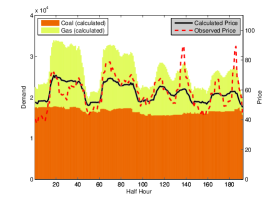
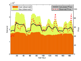
Figure 1: Comparison of the calculated and historical electricity price and energy mix when startup costs are excluded (i.e. set to zero).

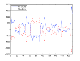
Figure 2: The difference between calculated and observed gas and coal production.

Calculated equilibrium prices and the energy mix with startup costs included are depicted in Figure 3. By comparing Figure 1 and Figure 3, we can see that the calculated equilibrium price captures the daily variations of the actually observed price much more closely. It correctly predicts some of the spikes, but also forecasts many false positives. Figure 4 shows that the inclusion of startup costs slightly improved the error in the energy mix calculation.

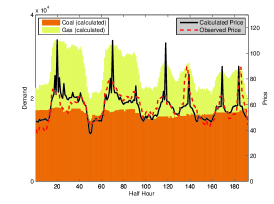
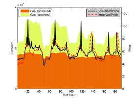
Figure 3: Comparison of the calculated and historical electricity price and energy mix when startup costs are included.

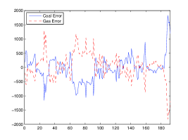
Figure 4: The difference between calculated and observed gas and coal production after including startup costs.

It is interesting to explore the conditions of the electricity grid at times when the spikes in the electricity price occur. A very descriptive parameter is standing reserve $SR\left(T_{j}\right)$, $j\in J$, defined as

(73) $$SR\left(T_{j}\right)=\sum_{p\in P}\sum_{l\in L}\sum_{r\in R^{p,l}}\left[W_{p,l,r}^{\left(2\right)}\left(T_{j}\right)-W_{p,l,r}^{\left(6\right)}\left(T_{j}\right)\right]\left[\overline{W}_{max}^{p,l,r}\left(T_{j}\right)-\overline{W}_{min}^{p,l,r}\left(T_{j}\right)\right],$$

which quantifies by how much the power plants that are currently running can increase their production before a new power plant must be turned on. Since most of the power plants have severe constraints on startup times, low standing reserve usually implies low stability of the electricity grid.

Figure 5 depicts the calculated standing reserve over the relevant time period. We can see that all price spikes occur when standing reserve is close to zero. In such situations, a new power plant must be turned on (and off quickly afterwards) to cover the temporary extra demand. Thus, the startup costs are spread over a very short period of time, and a high electricity price is required for such an action to be profitable. However, in reality, the times of a low standing reserve are very rare. The grid operator is responsible for providing a reliable electricity delivery and preventing times with a low standing reserve. This is achieved by incentivizing some of the power plants to start production even when it is not profitable for them. The costs of such actions are distributed among all market participants. How to include the grid operator in our model is discussed in the next section.

Figure 5: Standing reserve for the relevant time period.

In the remaining part of this section, we evaluate the error caused by using the continuous relaxation of Problem (PR). We follow the procedure described in Section 2.6. The MIQP error is depicted by a dashed line in Figure 6. To estimate the effect of numerical errors, we also calculated the QP error which is shown in Figure 6 as a solid line.

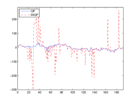
Figure 6: Error caused by considering Problem $\widetilde{PR}$ instead of Problem PR.

We can see from Figure 6 that $\left\|\sum_{c\in C}V_{c}^{*}+\sum_{p\in P}V_{p}^{*}\right\|_{\infty}\approx 400\>\text{MWh}$. Also in reality, production and consumption do not match exactly. The mismatch is reflected through changes in the power line frequency. In the UK, the nominal power line frequency is 50 Hz. The grid operator, called National Grid, is responsible for keeping the frequency within $\pm 1\%$ of the nominal power line frequency. We can see from Figure 6 that the largest errors occur at times when demand is high. Since the overall demand for electricity during the peak hours is approximately $40\>\text{GW}$ we can conclude that the error is within $\pm 1\%$ error bound.

The model presented in this paper neglects the losses of electricity in transmission and distribution lines. According to the World Bank the transmission and distribution losses in the UK account for approximately 7.5% (maximum 8.5% in 2004 and minimum 7.0% in 2010) of the total electricity production. The losses vary in time and can change for $\pm 1\%$.

Due to the reasons above, we believe that for the purpose of modeling realistic power prices, it is enough to consider the continuous relaxation of Problem (PR) and neglect binarity constraints.

4 Grid operator

In Section 2, we investigated how to include startup costs in our model. The calculated equilibrium price contained many spikes, which are in reality prevented by intervention of the grid operator. In times, when the standing reserve is low, the grid operator incentivizes additional power plants to turn on and thus help making the delivery of electricity more reliable. In this section we investigate how to incorporate the actions of the grid operator into our model.

4.1 Quadratic programming formulation

The costs of the grid operator’s actions that help to maintain a high reliability of the delivery of electricity are distributed among all market participants. All market participants are collectively penalized in the situations when the standing reserve is low. To include the penalization in our model, we propose a quadratic penalty function $\Upsilon\left(SR\left(T_{j}\right)\right)$ defined as

(74) $$\Upsilon\left(SR\left(T_{j}\right)\right):=\alpha\left(\max\left\{0,\beta-SR\left(T_{j}\right)\right\}\right)^{2},$$

where $\alpha>0$ and $\beta>0$ are used to describe a risk aversion of the grid operator. Parameter $\beta$ tells us at what level of the standing reserve does the grid operator start to take action. Parameter $\alpha$ tells us how much is the grid operator willing to incentivize the power plant to start production.

One can incorporate the grid operator into Problem (52) as

(75) $$\begin{array}[]{cl}\underset{x}{\text{max}}&-\pi^{\top}x-\frac{1}{2}x^{\top}Qx-\sum_{j\in J}\Upsilon\left(SR\left(T_{j}\right)\right)\\ \\ \text{s.t.}&Ax=a\\ \\ &Bx\leq b\\ \\ &\mu_{M}=0\end{array}$$

It might not be immediately clear, how to write the penalty term (74) in a quadratic programming framework. We can follow an approach that is widely used in the linear programming literature and introduce a decision variable $z\left(T_{j}\right)$ with the following constraints

(76) $$\begin{array}[]{rcl}z\left(T_{j}\right)&\geq&0\\ \\ z\left(T_{j}\right)&\geq&\beta-SR\left(T_{j}\right),\end{array}$$

which hold for each $j\in J$. The penalty function $\Upsilon\left(SR\left(T_{j}\right)\right)$ can be written as a function of $z\left(T_{j}\right)$ as

(77) $$\Upsilon\left(z\left(T_{j}\right)\right):=\alpha z\left(T_{j}\right)^{2},$$

which fits into the quadratic programming framework.

One can apply the procedure described in Section 2.6 to find a more convenient dual formulation of Problem (75).

4.2 Numerical results

In this section we investigate numerical results after inclusion of the grid operator. Calculated equilibrium prices and the energy mix and depicted in Figure 7. The figure on the left hand side depicts the calculated energy mix between coal and gas power plants, while the figure on the right hand side depicts the actually observed energy mix. Both figures contain also the spot price calculated by our model and the actually observed spot price. We set $\alpha=0.01$ and $\beta=1500$. Determination of the optimal standing reserve is a challenging problem, which has received a lot of attention in the literature (see [10] and [9] for example) and exceeds the scope this paper.

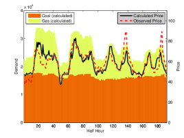
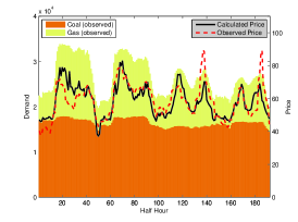
Figure 7: Comparison of the calculated and historical electricity price and energy mix with startup costs and the grid operator included.

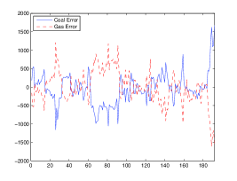
Figure 8: The difference between calculated and observed gas and coal production after including the grid operator.

By comparing Figure 3 and Figure 7, we can see that the calculated equilibrium electricity price in Figure 7 follows the daily variations much more closely. The calculated equilibrium electricity price does not contain any spikes, because the grid operator prevented them by managing the standing reserve. In our model, we assume that the players (and the grid operator) have a perfect demand forecast. However, in reality this is usually not the case. The grid operator is not able to predict the demand perfectly, and corrective actions are often required. When large corrective action is required at times close to delivery, then only a few (usually rather inefficient Open Cycle Gas Turbine) power plants are flexible enough to cover the demand, which causes spikes in the electricity price. Modeling of recursive actions exceeds the scope of this paper and is left for future work.

Figure 8 shows that the inclusion of the grid operator did not have any significant impact on the error in the energy mix.

Figure 9 shows the standing reserve after inclusion of the grid operator. The standing reserve never reaches zero since the grid operator prevents this by requiring new power plants to start production to ensure stability of the electricity grid. This makes the spot price smoother and significantly decreases the number of spikes.

Figure 9: Standing reserve for the relevant time period.

Figure 10 depicts the MIQP and QP errors after inclusion of the grid operator. By comparing Figure 6 and Figure 10, we can see that the inclusion of the grid operator has a small impact on the errors, which remained within $\pm 1\%$ error bound.

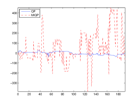
Figure 10: Error caused by considering Problem $\widetilde{PR}$ instead of Problem PR.

5 Conclusions

In this paper we proposed a tractable quadratic programming formulation for calculating the equilibrium term structure of electricity prices when the startup costs of power plants are included in the model. Through numerical simulations we showed that startup costs have a large impact on electricity prices. When startup costs are included in the model, the calculated spot electricity price during peak hours increased and during off-peak hours decreased. Moreover, startup costs are responsible for introducing frequent high spikes in the spot electricity price.

We observed that price spikes occur at times when the standing reserve in low. In reality, the times of a low standing reserve are rare, because of the intervention of the grid operator, who is responsible for providing a reliable electricity delivery and preventing times with a low standing reserve. We included the grid operator in our model in the second part of the paper. This significantly decreased the number of spikes. Moreover, the computed equilibrium electricity prices matched the historically observed prices very closely.

Numerical simulations were performed by modeling the realistic UK power grid consisting of a few hundred power plants. A tractable approach to estimate startup costs of power plants from their historical production was also proposed.

References

- [1] M. T. Barlow, A diffusion model for electricity prices, Mathematical Finance, 12 (2002), pp. 287–298.
- [2] Hendrik Bessembinder and Michael L. Lemmon, Equilibrium pricing and optimal hedging in electricity forward markets, Journal of Finance, 57 (2002), pp. 1347–1382.
- [3] Wolfgang Bühler, Risk premia of electricity futures: A dynamic equilibrium model, in Risk Management in Commodity Markets, John Wiley & Sons, Ltd., 2009, pp. 61–80.
- [4] Wolfgang Bühler and Jens Müller-Merbach, Valuation of electricity futures: Reduced-form vs. dynamic equilibrium models, Mannheim Finance Working Paper No. 2007-07, (2009).
- [5] René Carmona, Michael Coulon, and Daniel Schwarz, Electricity price modeling and asset valuation: a multi-fuel structural approach, Mathematics and Financial Economics, 7 (2013), pp. 167–202.
- [6] Les Clewlow and Chris Strickland, A multi-factor model for energy derivatives, Research Paper Series 28, Quantitative Finance Research Centre, University of Technology, Sydney, Dec. 1999.
- [7] , Valuing energy options in a one factor model fitted to forward prices, Research Paper Series 10, Quantitative Finance Research Centre, University of Technology, Sydney, Apr. 1999.
- [8] Gauthier De Maere d’Aertrycke and Yves Smeers, Liquidity Risks on Power Exchanges: a Generalized Nash Equilibrium model, 2012.
- [9] K. De Vos and J. Driesen, Dynamic operating reserve strategies for wind power integration, Renewable Power Generation, IET, 8 (2014), pp. 598–610.
- [10] E. Ela, B. Kirby, E. Lannoye, M. Milligan, D. Flynn, B. Zavadil, and M. O’Malley, Evolution of operating reserve determination in wind power integration studies, in Power and Energy Society General Meeting, 2010 IEEE, July 2010, pp. 1–8.
- [11] Isabel García, Claudia Klüppelberg, and Gernot Müller, Estimation of stable CARMA models with an application to electricity spot prices, Statistical Modelling, 11 (2011), pp. 447–470.
- [12] Paul R. Gribik, William W. Hogan, and Susan L. Pope, Market-clearing electricity prices and energy uplift, technical report, Harvard University, Cambridge, MA, Dec. 2007.
- [13] Inc. Gurobi Optimization, Gurobi Optimizer Reference Manual, 2014.
- [14] Ben Hambly, Sam Howison, and Tino Kluge, Modelling spikes and pricing swing options in electricity markets, Quantitative Finance, 9 (2009), pp. 937–949.
- [15] Scott M. Harvey and William W. Hogan, Market power and market simulations, technical report, Center for Business and Government, Harvard University, Cambridge, MA, July 2002.
- [16] Sam Howison and Michael C. Coulon, Stochastic behaviour of the electricity bid stack: From fundamental drivers to power prices, The Journal of Energy Markets, 2 (2009).
- [17] Julio J. Lucia and Eduardo Schwartz, Electricity prices and power derivatives: Evidence from the nordic power exchange, (2000).
- [18] D. Martinez, A methodology for the consideration of start-up costs into the marginal cost estimated with production cost models, in Electricity Market, 2008. EEM 2008. 5th International Conference on European, May 2008, pp. 1–10.
- [19] Thilo Meyer-Brandis and Peter Tankov, Multi-factor jump-diffusion models of electricity prices, International Journal of Theoretical and Applied Finance (IJTAF), 11 (2008), pp. 503–528.
- [20] M. Troha and R. Hauser, Calculation of a power price equilibrium, ArXiv e-prints, (2014).
- [21] , The existence and uniqueness of a power price equilibrium, ArXiv e-prints, (2014).
- [22] A.IsmaelF. Vaz and LuísN. Vicente, A particle swarm pattern search method for bound constrained global optimization, Journal of Global Optimization, 39 (2007), pp. 197–219.
- [23] Bingjie Zhang, P.B. Luh, E. Litvinov, Tongxin Zheng, and Feng Zhao, On reducing uplift payment in electricity markets, in Power Systems Conference and Exposition, 2009. PSCE ’09. IEEE/PES, Mar. 2009, pp. 1–7.