Observational constraints to a unified cosmological model

Abstract

We propose a phenomenological unified model for dark matter and dark energy based on an equation of state parameter $w$ that scales with the $\arctan$ of the redshift. The free parameters of the model are three constants: $\Omega_{b0}$, $\alpha$ and $\beta$. Parameter $\alpha$ dictates the transition rate between the matter dominated era and the accelerated expansion period. The ratio $\beta/\alpha$ gives the redshift of the equivalence between both regimes. Cosmological parameters are fixed by observational data from Primordial Nucleosynthesis (PN), Supernovae of the type Ia (SNIa), Gamma-Ray Bursts (GRB) and Baryon Acoustic Oscillations (BAO). The calibration of the 138 GRB events is performed using the 580 SNIa of the Union2.1 data set and a new set of 79 high-redshift GRB is obtained. The various sets of data are used in different combinations to constraint the parameters through statistical analysis. The unified model is compared to the $\Lambda$CDM model and their differences are emphasized.

PACS numbers

95.35.+d, 95.36.+x, 98.80.Es

I Introduction

The recent technological improvement in the space observations deeply altered Cosmology. In the end of the 90’s, the measurement of the luminosity distance of type Ia supernovae (SNIa) unveiled an accelerating cosmic expansion at recent times Riess et al. (1998); Perlmutter et al. (1999). This result was later confirmed by other works using different sets of data Weinberg et al. (2013) such as the cosmic microwave background radiation (CMB) Abergel et al. (2014), baryon acoustic oscillations (BAO) Percival et al. (2010); Anderson et al. (2014) and even the relatively recent Gamma-Ray burst (GRB) data Wei and Nan Zhang (2009); Schaefer (2007); Amati et al. (2002). As long as one assumes a homogeneous and isotropic cosmological background, the cosmic acceleration at low redshifts seems an indisputable observational truth.

The simplest theoretical way of describing cosmic acceleration is through the cosmological constant $\Lambda$, a negative energy density uniformly distributed throughout the cosmos. The resulting $\Lambda$CDM cosmological model Weinberg (2008) is robust when confronted to observational data, although it is not a comfortable solution mainly due to the lack of a clear interpretation of the physical meaning of $\Lambda$ in terms of the known fundamental interactions. This very fact relegates $\Lambda$ to the mysterious “dark sector” of the universe. It is completed by the gravitationally bound cold dark matter (CDM), whose nature is also unknown.

In face of these two unexplained components, one is tempted to unify them in a single dark fluid. This unified model would have to be capable of accelerating the universe at recent times and also provide a dust dominated epoch toward the past in order to accommodate structure formation. This is our motivation to introduce the Unified Model (UM) described in Sect. II.1. There is a plethora of cosmological models based on the same idea Bertacca et al. (2010); they are build either based on theoretical motivations Peebles and Vilenkin (1999); Kamenshchik et al. (2001); Bento et al. (2002); Padmanabhan and Choudhury (2002); Scherrer (2004); Giannakis and Hu (2005); Bertacca et al. (2007); Giannantonio and Melchiorri (2006); Santos et al. (2006); Radicella and Pavón (2014); Sharif et al. (2012) or on phenomenological ones Makler et al. (2003a, b); Alcaniz et al. (2003); Balbi et al. (2007); Pietrobon et al. (2008); Ishida et al. (2008); Giostri et al. (2012); Fabris et al. (2011); Wang et al. (2013). Our model is built on phenomenological grounds.

The UM is a dynamical model developed from a specific functional form chosen for the parameter $w$ of the equation of state $p=w\rho$, where $p$ is the pressure related to the cosmic component of density $\rho$: $w$ is given in terms of the $\arctan$ function. This way, the universe filled with the unified fluid passes smoothly from a matter-like behavior $(w\simeq 0)$ to a dark-energy-like dynamics $(w\simeq-1)$. This property is justified theoretically once the history of the universe demands a matter-dominated era with decelerated expansion ($2\lesssim z\lesssim 10000$) followed by an accelerated period dominated by dark energy ($z\lesssim 2$) Ellis et al. (2012). Our goal is to treat dark matter and dark energy on the same footing.

The unified scenario for the dark components is meaningful only if one can constraint the free parameters of the Unified Model by using a large number of observational data. For this end, we will use the already mentioned SNIa, BAO and GRB data plus information on the baryon density parameter $\Omega_{b0}$ coming from primordial nucleosynthesis (PN) data.

We used Union2.1 compilation Suzuki et al. (2012) for obtaining the distance modulus $\mu$ of the supernovae as a function of their redshift $z$. For the GRB, we employed data in Ref. Liu and Wei (2014), which include 29 GRB in addition to the set of 109 GRB of Ref. Wei (2010). Also, we payed special attention to the construction of the calibration curve of the GRB. The procedure involved an interpolation to the points in the plot of $\mu$ as function of $z$. We noticed that the common interpolation methods, such as linear and cubic interpolation techniques, are not the best-quality ones. In fact, Akima’s method Akima (1970) is the one which provides a curve that naturally connects the observational points without bumps or discontinuities. We devoted special care to the GRB data as they rise as new good candidates for standard candles at very high redshifts, with great potential of revealing additional cosmological information.

The paper is organized as follows. Sect. II presents our Unified Model (UM) for the dark sector of the universe; in addition, the basic equation of the $\Lambda$CDM model are reviewed. This prepares the ground for data fitting aiming to constraint the free parameters of both UM and $\Lambda$CDM. The statistical treatment is performed in Sect. III after the cosmological data sets used in our analysis have been discussed. The physical consequences of the data fit for the various combinations of data (PN, SNIa, GRB and BAO) are also addressed in Sect. III and further discussed in Sect. IV, where we also point out our final comments.

II Cosmological set up

This section presents the two cosmological models that are constrained by observational data in this paper. The first one is a phenomenological model that we call Unified Model (UM). The second one is the fiducial $\Lambda$CDM model, considered here for the sake of comparison.

II.1 Unified model

Our framework will be a flat universe filled with baryonic matter and a unified component of dark matter and dark energy. The Hubble function for this model is

$$H=H_{0}\sqrt{\Omega_{\text{U}}\left(z,\alpha,\beta\right)+\Omega_{b0}\left(1+z\right)^{3}},$$ (1)

where $\Omega_{\text{U}}\left(z,\alpha,\beta\right)$ is the density parameter of the unified fluid,

$$\Omega_{\text{U}}\left(z\right)=\Omega_{\text{U}0}\exp\left\{\int_{0}^{z}3\dfrac{\left[1+w_{\text{U}}\left(z^{\prime}\right)\right]}{1+z^{\prime}}dz^{\prime}\right\},$$

which is subjected to the constraint

$$\Omega_{\text{U}0}+\Omega_{b0}=1$$ (2)

and depends on the redshift $z$ and three free parameter $\Omega_{b0}$, $\alpha$ and $\beta$ to be determined from adjustment to the available observational data.

The parameter $w_{\text{U}}$ of the equation of state is a function of $z$ and describes the transition from the matter dominated dynamics to the acceleration domination epoch. It is convenient to define Bruni et al. (2013)

$$w_{\text{U}}=\dfrac{1}{\pi}\arctan\left(\alpha z-\beta\right)-\dfrac{1}{2}.$$ (3)

The idea to propose a phenomenological parameterization which unifies the dark components is not new. For instance, in the works Ishida et al. (2008), Giostri et al. (2012) the authors use an expression exhibiting plots resembling those built with Eq. (3); however, there is an important conceptual difference between their reasoning and ours. Whereas in this paper we adopt a dynamical approach, the authors of Ishida et al. (2008), Giostri et al. (2012) use a kinematic one. The advantage of a kinematic model in which one chooses to parameterize the deceleration parameter $q$ in terms of the redshift $z$ – as that of Ref. Giostri et al. (2012) – is that very few assumptions on the nature of the dark components are taken a priori. On the other hand, dynamical models parameterizing $w\left(z\right)$ are more physical in the sense that they enable a meaningful perturbation theory (once they presuppose Einstein’s equation of gravity and standard cosmological assumptions).

Parameter $\alpha$ gives the transition rate between the decelerated expansion and the recent accelerated phase of the universe’s evolution. Parameter $\beta$ provides the value for $w_{\text{U}}$ today (null redshift). Moreover,

$$z_{\text{eq}}=\dfrac{\beta}{\alpha}$$ (4)

is the redshift corresponding to the equivalence between the dark energy and the dark matter energy densities. This expression is obtained by taking $w_{\text{U}}=-1/2$, the average of the values $w=0$ and $w=-1$.

Fig. 1a shows that the larger is $\alpha$ the greater is the transition rate (if $\beta$ is kept constant). Fig. 1b illustrates the fact that the value of the redshift of equivalence grows with $\beta$ (for a given $\alpha$).

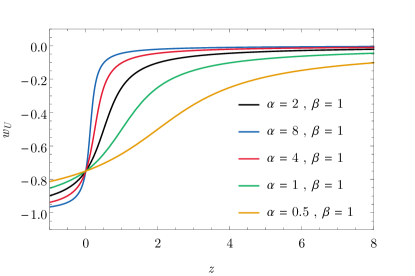
(a)

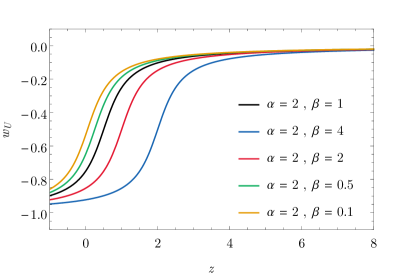
(b)

Figure 1: Curves of $w_{\text{\text{U}}}$ as a function of $z$ for different values of parameters $\alpha$ and $\beta$ — see Eq. (3).

II.2 $\Lambda$CDM

We shall fit the concordance $\Lambda$CDM model to the observations using the same data sets and techniques applied to our unified model for comparison.

The $\Lambda$CDM Hubble function for the flat universe is:

$$H\left(z\right)=H_{0}\sqrt{(\Omega_{b0}+\Omega_{d0})\left(1+z\right)^{3}+\left(1-\Omega_{b0}-\Omega_{d0}\right)},$$ (5)

where $\Omega_{b0}$ is the density parameter for the baryonic matter and $\Omega_{d0}$ is the density parameter for the dark matter component. In the $\Lambda$CDM cosmology, the constant $\Omega_{\Lambda}=(1-\Omega_{b0}-\Omega_{d0})$ is the density parameter of the dark energy, interpreted as a cosmological constant. We define the effective equation of state parameter $w_{\text{dark}}$ for the $\Lambda$CDM model by the ratio of the pressure to the energy density of the dark components:

$$w_{\text{dark}}=-\frac{\Omega_{\Lambda}}{\Omega_{d0}\left(1+z\right)^{3}+\Omega_{\Lambda}}\,.$$ (6)

Analogously to what we have done for the unified model, the equivalence redshift $z_{\text{eq}}$ is the solution to $w_{\text{dark}}(z_{\text{eq}})=-1/2$. Then:

$$z_{\text{eq}}=\left(\dfrac{1-\Omega_{b0}-\Omega_{d0}}{\Omega_{d0}}\right)^{1/3}-1.$$ (7)

The above formulas will be useful in Sec. III when we obtain parameters $\Omega_{b0}$ and $\Omega_{d0}$ using the observational data.

III Cosmological data sets, analysis and results

The free parameters in Eqs. (1) and (5) will be estimated using four different data sets: Primordial Nucleosynthesis, Supernovae of the type Ia, Gamma-Ray Bursts and Baryon Acoustic Oscillations.

III.1 Primordial Nucleosynthesis data

According to the Big Bang model, the nuclei of the light elements — hydrogen (H), deuterium (D), ³He, ⁴He e ⁷Li — were created in the first minutes of the Universe during a phase known as the primordial nucleosynthesis Kirkman et al. (2003). The abundances of these light elements depend on the present-day value of the baryon density parameter $\Omega_{b0}$ and on the Hubble constant $H_{0}$ Pettini and Cooke (2012). In fact, it is possible to obtain $\Omega_{b0}h^{2}$ through a precise measurement of the primordial abundance ratio for any two light nuclei species.

Among those nuclei formed during the primordial nucleosynthesis, the simplest to be measure is the deuterium to hydrogen abundance ratio $\left(D/H\right)$ O’meara et al. (2006). Ref. Adams (1976) suggests to determine this ratio using information from a special type of high-redshift quasar (QSO), more specifically through damped Lyman alpha systems (DLA) spectra Kirkman et al. (2003); Tytler et al. (1996); Burles and Tytler ; O’meara et al. (2001). The deuterium to hydrogen abundance ratio was given as $(D/H)=\left(2.535\pm 0.05\right)\times 10^{-5}$ by Ref. Pettini and Cooke (2012) This result follows from the DLA QSO SDSS J1419+0829 spectrum. The above value for $(D/H)$ leads to

$$\Omega_{b0}h^{2}=0.0223\pm 0.0009~{}.$$ (8)

Refs. Riess et al. (2011) and Freedman et al. (2012) discuss measurements of the Hubble constant $H_{0}$ with a negligible dependence on the cosmological model. These two sources enable one to obtain the normalized Hubble constant $h$ in Eq. (8) as:

$$\left\{\begin{array}[c]{l}h_{\text{R}}=0.738\pm 0.028\\ h_{\text{F}}=0.743\pm 0.015(\text{sta})\pm 0.021\left(\text{sys}\right)\end{array}\right.\begin{array}[c]{l}\text{(Riess);}\\ \text{(Freedman).}\end{array}$$ (9)

On the order hand, the $H_{0}$ measured for Planck satellite Abergel et al. (2014) indicates $h=0.673\pm 0.012$. So, there is a noticeable $2.5\sigma$ discrepancy between the values for $h$ given by Riess and Freedman and the one measured by Planck satellite. In this work, we shall adopt a conservative stance and use $h=0.74$. Nevertheless we use $\sigma_{h}=0.07$ as uncertainty in order to accommodate Planck’s value with a confidence interval of $1\sigma$. Using the data in (9) and Eq. (8), one can estimate the baryon density parameter as $\Omega_{b0}^{\,\text{PN}}=\left(0.0407\pm 0.0079\right)$.

III.2 SNIa data

The supernovae are super-massive star explosions with intense luminosity. Among them, type Ia supernovae (SNIa) are the most important for cosmology since they can be taken as standard candles due to their characteristic luminosity curves.

In order to estimate the cosmological parameters of the unified model, we will employ the 580 SNIa compilation available in Ref. Suzuki et al. (2012) by the Supernova Cosmology Project (SCP). Union2.1 data set presents the redshift $z$ of each supernova and the related distance modulus $\mu$ accompanied by its uncertainty $\sigma_{\mu}$.

The distance modulus $\mu$ is a logarithmic function of the normalized luminosity distance $d_{h}$:

$$\mu(z;\vec{\theta},\mathcal{M})=5\log d_{\text{h}}(z;\vec{\theta})+\mathcal{M\,},$$ (10)

with

$$d_{\text{h}}\equiv\dfrac{H_{0}}{c}d_{\text{L}}=\left(1+z\right)H_{0}\int_{0}^{z}\dfrac{dz^{\prime}}{H(z^{\prime};\vec{\theta}\,)}\,.$$ (11)

$\mathcal{M}$ is a constant depending on the Hubble constant $H_{0}$, the speed of light $c$ and the absolute magnitude of the standard supernova in the regarded band Amendola et al. (2007). $\vec{\theta}$ is the vector of parameters for the particular cosmological model under consideration. We shall not discuss the quantities encapsulated in $\mathcal{M}$ since they are not of our concern here; in fact, $\mathcal{M}$ is marginalized in the statistical treatment of the data. In fact, we define

$$\chi_{\text{S+N}}^{2}(\vec{\theta}\,)=\chi_{\text{SN,}m}^{2}(\vec{\theta}\,)+\chi_{\text{PN}}^{2}~{}$$ (12)

where

$$\chi_{\text{PN}}^{2}=\dfrac{\left(\Omega_{b0}-\Omega_{b0}^{\,\text{PN}}\right)^{2}}{\left(\sigma_{\Omega_{b0}^{\,\text{PN}}}\right)^{2}}~{},$$ (13)

and the function $\chi_{\text{SN,}m}^{2}$ comes from the $\chi_{\text{SN}}^{2}$ of Union2.1 supernovae data,

$$\chi_{\text{SN}}^{2}(\vec{\theta},\mathcal{M})=\sum_{i=1}^{580}\dfrac{\left[\mu_{i}-5\log d_{h}(z_{i};\vec{\theta}\,)-\mathcal{M}\right]^{2}}{\sigma_{\mu_{i}}^{2}},$$ (14)

after analytic marginalization of the parameter $\mathcal{M}$ Goliath et al. (2001).

We estimate the vector of parameters $\vec{\theta}_{\text{UM}}=\left(\Omega_{b0},\alpha,\beta\right)$ and $\vec{\theta}_{\Lambda\text{CDM}}$ $=\left(\Omega_{b0},\Omega_{d0}\right)$ by minimizing $\chi_{\text{S+N}}^{2}(\vec{\theta})$ for the UM and $\Lambda$CDM model. The values of the parameters for both models are found in Table 3. The best-fit parameters are used to build distance moduli curves for both models. The upper part of Fig. 2 show how well UM vs. $\Lambda$CDM fit the data. The residual plots are at the lower part of Fig. 2. Confidence region graphs (with $1\sigma$, $2\sigma$ and $3\sigma$) are displayed in Fig. 3.

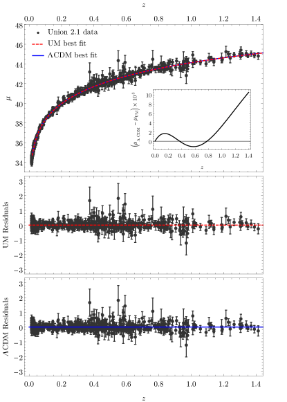
Figure 2: SNIa data and the distance modulus curves built with the best-fit values of UM and $\Lambda$CDM (top). The curve $\mu(z)$ for UM almost coincides with the one for $\Lambda$CDM; the small differences between $\mu_{\text{UM}}$ and $\mu_{\Lambda\text{CDM}}$ are emphasized in the plot of $(\mu_{\Lambda\text{CDM}}-\mu_{\text{UM}})\times 10^{3}$ as a function of $z$. The residual plots for UM (center) and $\Lambda$CDM (bottom) are also show.

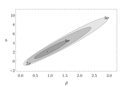
(a) Unified Model

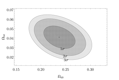
(b) $\Lambda$CDM

Figure 3: (a) UM: 68.3%, 95.4% and 99.7% confidence regions of the $(\beta,\alpha)$ plane from SNIa data combined with the constraint from PN. (b) $\Lambda$CDM model: 68.3%, 95.4% and 99.7% confidence regions of the $(\Omega_{d0},\Omega_{b0})$ plane from SNIa data combined with the constraint from PN. Confidence contours include statistical and systematic errors in both cases.

III.3 GRB data

The SNIa data provide us with reliable cosmological information till redshifts of the order of $1.7$ (cf. Riess et al. (2001)). On the other hand, cosmic microwave background anisotropy measurements permit us to access information about the large scale universe at $z\sim 1000$ Hu et al. (1995). In between, there is a large redshift interval observationally inaccessible; scientific community is making great effort to collect astronomical data to fill in this gap. Perhaps the most promising candidates for this scope are the Gamma-Ray Bursts. It is expected that a fraction $\gtrsim 50\%$ of the observed GRB have $z>5$ and the redshift values of these objects may be as large as $10$ or even greater Bromm and Loeb (2002).

Even though we do not fully understand GRB emission mechanism, they are considered excellent candidates to standard candles because of their intense brightness Wei and Nan Zhang (2009), Li et al. (2011). That is the reason why many authors have been proposing empirical luminosity correlation functions that standardize GRB as distance indicators Amati et al. (2002); Ghirlanda et al. (2004a); Liang and Zhang (2005); Firmani et al. (2005).

An additional problem to the use of GRB is the so called circularity problem. Unlike what happens in the supernovae case, there is no data set that is completely model independent and which could be used to calibrate GRB distance curves Wei and Nan Zhang (2009), Schaefer (2007). A number of different statistical methods were suggested to overcome this model dependence; e.g. see Refs. Wei and Nan Zhang (2009); Wei (2010); Graziani (2011); Wang (2008); Ghirlanda et al. (2004b, 2006); Li et al. (2008); Liang and Zhang (2006); Liang et al. (2008).

This work make use of the 138 Gamma-Ray Bursts compiled in Ref. Liu and Wei (2014). They were calibrated according to the method described in Ref. Wei (2010), which tries to eliminate model dependence. Two different groups of GRB were considered: the low-redshift set has $z<1.4$; the high-redshift one presents events with $z>1.4$.

The distance modulus of the low-redshift GRB were determined using the SNIa data in the following way. We built the plot of the distance modulus versus the redshift for the 580 supernovae of the Union2.1 data set. The supernovae with the same redshift had their distance modulus values averaged. The points in the plot $z\times\mu$ were interpolated to provide a function $\mu=\mu\left(z\right)$ with domain $0\leq z\leq 1.4$. There are many interpolation techniques such as linear, cubic and Akima’s interpolations Akima (1970). We used these three methods and chose the last one for building the function $\mu\left(z\right)$ because Akima’s technique is the one giving a curve that intercepts the points in a more smooth and natural way – see Appendix A. With these SNIa low-redshift $\mu\left(z\right)$ it is possible to estimate the distance modulus of each one of the 59 low-redshift GRB. These values of $\mu$ are then substituted in

$$\mu=5\log_{10}\dfrac{d_{\text{L}}}{\text{Mpc}}+25$$ (15)

to give the associated luminosity distances $d_{L}$. They, in turn, appear in the expression for the isotropically radiated equivalent energy:

$$E_{\text{iso}}=\dfrac{4\pi S_{\text{bolo}}d_{L}^{2}}{1+z},$$ (16)

where $S_{\text{bolo}}$ is the GRB observed bolometric fluency. In the work Amati et al. (2002), Amati noticed the correlation between the energy peak of the GRB spectrum ($E_{\text{p}}$) and the isotropically radiated energy ($E_{\text{iso}}$), formulating the equation:

$$\log_{10}\dfrac{E_{\text{iso}}}{\text{erg}}=\lambda+b\log_{10}\dfrac{E_{\text{p}}}{300~{}\text{keV}},$$ (17)

which is known as the Amati’s relation. We determine parameters $\lambda$ and $b$ by using the low-redshift GRB data set, with the $E_{\text{p}}$ data available in Ref. Liu and Wei (2014) and the $E_{\text{iso}}$ obtained from the SNIa calibration curve. Parameters $\lambda$ and $b$ are obtained from a linear fit to the Amati’s relation. The usual linear fit procedures in astronomy are the ordinary least-squares regression of the dependent variable $Y$ against the independent variable $X$ – OLS(Y$|$X) – and the ordinary least-squares of $X$ on $Y$ – OLS(X$|$Y). However, if there is a domain within which occurs an intrinsic scattering of the data with respect to the individual uncertainties, it is preferable to use the OLS bisector method, as described in Ref. Isobe et al. (1990). Following the procedure in this reference, we performed linear regressions using the three methods above; the values obtained for the parameters $b$ and $\lambda$ of the Amati’s relation are displayed in Table 1; the straight lines built from those parameters are shown in Fig.4.

Table 1: Parameter $b$ and $\lambda$ of the Amati’s relation.

Method $b$ $\sigma_{b}$ $\lambda$ $\sigma_{\lambda}$ OLS(X$|$Y) $1.564$ $0.084$ $52.74$ $0.06$ OLS(Y$|$X) $1.861$ $0.099$ $52.79$ $0.06$ OLS bisector $1.703$ $0.053$ $52.77$ $0.06$

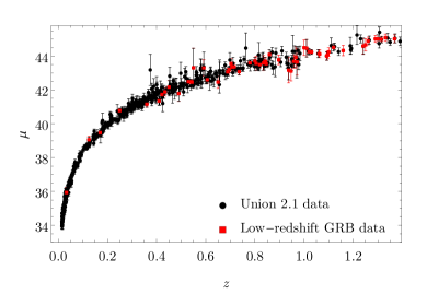
(a)

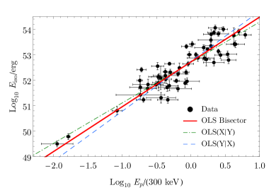
(b)

Figure 4: (a) $\mu\left(z\right)$ points for the Union2.1 SNIa data set (in black) and low-redshift GRB data (red). (b) Linear regression procedures for determining parameters $b$ and $\lambda$ in the relation by Amati.

We decided to adopt the values of $\lambda$ and $b$ given by the OLS bisector method once the intrinsic dispersion of the data is dominant over the observational errors. Then, we calculated the quantity $\log_{10}E_{\text{iso}}$ for the high-redshifts GRB and their distance modulus

$$\mu=\dfrac{5}{2}\log_{10}\dfrac{E_{\text{iso}}}{\operatorname{erg}}+\dfrac{5}{2}\log_{10}\dfrac{\left(1+z\right)}{4\pi S_{\text{bolo}}}+25$$ (18)

with an associated uncertainty

$$\sigma_{\mu}=\sqrt{\left(\dfrac{5}{2}\sigma_{\log_{10}E_{\text{iso}}}\right)^{2}+\left(\dfrac{5}{2\ln 10}\dfrac{\sigma_{S_{\text{bolo}}}}{S_{\text{bolo}}}\right)^{2}}.$$ (19)

The uncertainty related to $\log_{10}E_{\text{iso}}$ is given by:

$$\sigma_{\log_{10}E_{\text{iso}}}^{2} = \sigma_{\lambda}^{2}+\left(\dfrac{b}{\ln 10}\dfrac{\sigma_{E_{\text{p}}}}{E_{\text{p}}}\right)^{2}+$$ (20)

$$+\left(\sigma_{b}\log_{10}\dfrac{E_{\text{p}}}{300~{}\text{keV}}\right)^{2}+\sigma_{E_{\text{sys}}}^{2}.$$

This equation is obtained from Amati’s relation through error propagation. We also added the contribution of the systematic error $\sigma_{E_{\text{sys}}}$ coming from extra dispersion in the luminosity relations. This systematic error is a free parameter and can be estimated by imposing $\chi_{\text{red}}^{2}=1$ on the curve fitting to the luminosity plots. This was done in Ref. Schaefer (2007), and the value obtained is: $\sigma_{E_{\text{sys}}}^{2}=0.39$.

After performing the GRB calibration using Union2.1 SNIa data, one obtains a set of values for the distance modulus $\mu\left(z\right)$ (and its uncertainty $\sigma_{\mu}$) for 79 high-redshift GRB. This set of values for $\mu\left(z\right)\pm\sigma_{\mu}$ is shown in Appendix B. It is used to build the function $\chi_{\text{GRB}}^{2}$:

$$\chi_{\text{GRB}}^{2}(\vec{\theta},\mathcal{M})=\sum_{i=1}^{79}\dfrac{\left[\mu_{i}-5\log\frac{d_{L}(z_{i};\vec{\theta}\,)}{\text{Mpc}}-25\right]^{2}}{\sigma_{\mu_{i}}^{2}}.$$ (21)

Now we use as input to our statistical treatment the three sets of data discussed so far (Union2.1 data; the value of $\Omega_{b0}^{\,\text{PN}}$ coming from PN; and, the 79 high-redshift GRB data duly calibrated) to estimate the cosmological parameters.

The best-fit values and single-parameter estimates are displayed in Table 3. Fig. 5 exhibits the double-parameter estimates with $1\sigma$, $2\sigma$ e $3\sigma$ confidence regions.

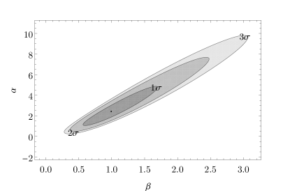
(a) Unified Model

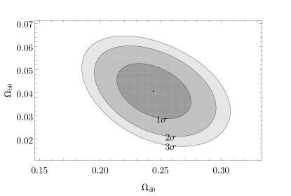
(b) $\Lambda$CDM

Figure 5: (a) UM: 68.3%, 95.4% and 99.7% confidence regions of the $(\beta,\alpha)$ plane from SNIa and PN plus high-redshift GRB data. (b) $\Lambda$CDM model: 68.3%, 95.4% and 99.7% confidence regions of the $(\Omega_{d0},\Omega_{b0})$ plane from SNIa data combined with PN and GRB data. Confidence contours include statistical and systematic errors in both cases.

III.4 BAO data

Before the last scattering, the baryon-photon plasma weakly coupled oscillated due to a competition between the gravitational collapse and the radiation pressure Ellis et al. (2012). According to Hu and Sugiyama (1996), the velocity of the resulting sound waves in the plasma is $c_{s}=1/\sqrt{3(1+3\rho_{b}/4\rho_{\gamma})}$. The stagnation of these waves after the decoupling lead to an increase of the baryon density at the scales corresponding to the distance covered by the acoustic wave until the decoupling time. This effect produces a peak of baryon acoustic oscillation (BAO) in the galaxy correlation function. BAO peaks data present very small systematic uncertainties when compared to the other cosmological data sets Percival et al. (2010); Albrecht et al. (2006). This is clearly an advantage to be used.

The baryon release marks the end of the Compton drag epoch and occurs at the redshift $z_{\text{drag}}\simeq 1059$ Abergel et al. (2014). The sound horizon $r_{s}$ determines the location of the length scale of the BAO peak. It is given by:

$$r_{s}\left(z_{\text{drag}}\right)=\dfrac{1}{\sqrt{3}}\int_{z_{\text{drag}}}^{\infty}\dfrac{c~{}dz}{\bar{H}\left(z\right)\sqrt{1+\tfrac{3}{4}\tfrac{1}{\left(1+z\right)}\tfrac{\Omega_{b0}}{\Omega_{\gamma 0}}}}.$$ (22)

The original Hubble function of the unified model, Eq.(1), must be modified to

$$\bar{H}\left(z\right) = H_{0}\Big{[}\Omega_{\text{U}}\left(z,\alpha,\beta\right)+$$ (23)

$$+\Omega_{b0}\left(1+z\right)^{3}+\Omega_{r0}\left(1+z\right)^{4}\Big{]}^{1/2},$$

in order to include the radiation-like term $\Omega_{r0}\left(1+z\right)^{4}$. This is necessary here because we are dealing with the $z>1000$, corresponding to the baryon-photon decoupling epoch, when the radiation was by no means negligible. The fact that $\lim_{z\rightarrow 0}\bar{H}\left(z\right)=H\left(z\right)$ guarantees that $\bar{H}\left(z\right)$ describes the same unified model we have been discussing from the beginning of the paper.

For the sake of comparison, we shall study the sound horizon $r_{s}$ for the $\Lambda$CDM model. The Hubble function for this case is:

$$\bar{H}\left(z\right) = H_{0}\Big{[}\left(1-\Omega_{b0}-\Omega_{d0}-\Omega_{r0}\right)+$$

$$+\left(\Omega_{b0}+\Omega_{d0}\right)\left(1+z\right)^{3}+\Omega_{r0}\left(1+z\right)^{4}\Big{]}^{1/2}.$$

The density parameter $\Omega_{r0}$ describes the contributions from the photons as well as that from the ultra-relativistic neutrinos. In accordance with Komatsu et al. (2009); Ichikawa et al. (2008),

$$\Omega_{r0}=\Omega_{\gamma 0}\left(1+0.2271N_{\text{eff}}\right),$$ (25)

where $N_{\text{eff}}=3.046$ is the effective number of neutrinos. The present-day value of the photon density parameter is $\Omega_{\gamma 0}=5.46\times 10^{-6}$, cf. Ref. Olive et al. (2014).

When we substitute (23) into (22), the sound horizon turns out to be a function of the free parameters $\alpha$ and $\beta$ present in our unified model: $r_{s}=r_{s}\left(\alpha,\beta\right)$. The sound horizon is then used to constraint $\alpha$ and $\beta$. This is done in the following way. BAO data allow us to obtain the angular diameter distance $D_{A}\left(z\right)$, achieved from the observation of the clustering perpendicular to the line of sight, and the Hubble function $H\left(z\right)$, measured through the clustering along the line of sight. However, $D_{A}\left(z\right)$ and $H\left(z\right)$ are not obtained independently, but through the distance scale ratio Farooq (2013)

$$d_{z}=\dfrac{r_{s}(z_{\text{drag}},\vec{\theta}\,)}{D_{v}(z,\vec{\theta}\,)},$$ (26)

where

$$D_{v}(z,\vec{\theta}\,)=\left[\left(1+z\right)^{2}D_{A}^{2}(z,\vec{\theta}\,)\dfrac{cz}{H(z^{\prime},\vec{\theta}\,)}\right]^{1/3}$$ (27)

is the effective distance ratio, and

$$D_{A}(z,\vec{\theta}\,)=\dfrac{1}{\left(1+z\right)}\int\dfrac{cdz^{\prime}}{H(z^{\prime},\vec{\theta}\,)}~{}.$$ (28)

We perform a data fit to the three values measured for the distance scale ratio $d_{z}$ — see Table 2. These are non-correlated BAO peaks data.

Table 2: BAO data.

Survey	$z$	$d_{z}$	Reference
6dFGS	$0.106$	$0.336\pm 0.015$	Beutler et al. (2011)
Boss	$0.32$	$0.1181\pm 0.0023$	Anderson et al. (2014)
Boss	$0.57$	$0.07261\pm 0.00071$	Anderson et al. (2014)

Function $\chi_{\text{BAO}}^{2}$,

$$\chi_{\text{BAO}}^{2}(\vec{\theta}\,)=\sum_{i=1}^{3}\dfrac{1}{\sigma_{i}^{2}}\left[d_{z,i}-\dfrac{r_{s}(z_{\text{drag}},\vec{\theta}\,)}{D_{v}(z_{i},\vec{\theta}\,)}\right]^{2}~{},$$ (29)

is calculated using the data in Table 2. We add to this function the expression for $\chi_{\text{S+N}}^{2}$, Eq. (12), so that we take into account BAO data together with SNIa and PN data sets. By minimizing the complete $\chi^{2}$, one finds the best-fit values and the single-parameter estimates shown in Table 3. Fig. 6 displays the confidence regions related to the two-parameter estimates.

According to the values shown in Table 3, the set including SNIa, PN and BAO is rather restrictive in comparison with the results obtained with SNIa and PN only. By considering the BAO peaks in the statistical treatment we reduced considerably the $1\sigma$-confidence interval of the single-parameter estimates.

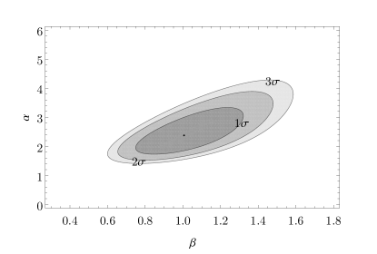
(a) Unified Model

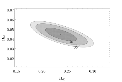
(b) $\Lambda$CDM

Figure 6: (a) UM: 68.3%, 95.4% and 99.7% confidence regions of the $(\beta,\alpha)$ plane from SNIa plus PN and BAO. (b) $\Lambda$CDM model: 68.3%, 95.4% and 99.7% confidence regions of the $(\Omega_{d0},\Omega_{b0})$ plane from the combination (SNIa + PN + BAO). Confidence contours include statistical and systematic errors in both cases.

Table 3: Parameters of the UM and of the $\Lambda$CDM model obtained through the fits to the various sets of data. Uncertainties of $z_{\text{eq}}$ are calculated by the Monte Carlo approach Watt and Thorne (2012). All statistical analysis include SNIa and PN data: they are taken as a basis for comparison with the results coming from the addition of GRB and BAO data.

Set	Parameter	PN+SNIa		PN+SNIa+GRB		PN+SNIa+BAO		PN+SNIa+GRB+BAO
		Best-fit	Single-parameter	Best-fit	Single-parameter	Best-fit	Single-parameter	Best-fit	Single-parameter
UM	$\alpha$	2.1	$2.1_{-1.2}^{+1.6}$	2.4	$2.6_{-1.1}^{+1.5}$	2.4	$2.39_{-0.37}^{+0.43}$	2.4	$2.42_{-0.38}^{+0.44}$
	$\beta$	0.92	$0.95_{-0.34}^{+0.45}$	0.99	$1.05_{-0.32}^{+0.45}$	1.0	$1.02_{-0.14}^{+0.15}$	0.99	$1.01_{-0.14}^{+0.15}$
	$\Omega_{b0}$	0.041	$0.0412_{-0.0085}^{+0.0073}$	0.041	$0.0412_{-0.0085}^{+0.0073}$	0.041	$0.0401_{-0.0080}^{+0.0070}$	0.041	$0.0393_{-0.0080}^{+0.0070}$
	$z_{\text{eq}}$	0.45	$0.377_{-0.066}^{+0.103}$	0.41	$0.366_{-0.050}^{+0.069}$	0.42	$0.409_{-0.046}^{+0.058}$	0.41	$0.404_{-0.049}^{+0.048}$
	$\chi^{2}_{\text{red}}$	0.97	-	0.94	-	0.96	-	0.94	-
$\Lambda$CDM	$\Omega_{d0}$	0.24	$0.237_{-0.021}^{+0.021}$	0.24	$0.244_{-0.020}^{+0.020}$	0.24	$0.237_{-0.020}^{+0.021}$	0.24	$0.243_{-0.020}^{+0.020}$
	$\Omega_{b0}$	0.041	$0.0407_{-0.0079}^{+0.0078}$	0.041	$0.0407_{-0.0079}^{+0.0078}$	0.044	$0.0443_{-0.0044}^{+0.0045}$	0.044	$0.0435_{-0.0043}^{+0.0044}$
	$z_{\text{eq}}$	0.45	$0.444_{-0.054}^{+0.058}$	0.43	$0.430_{-0.054}^{+0.050}$	0.45	$0.442_{-0.053}^{+0.055}$	0.43	$0.429_{-0.052}^{+0.049}$
	$\chi^{2}_{\text{red}}$	0.97	-	0.94	-	0.96	-	0.94	-

III.5 PN, SNIa, GRB and BAO data sets

Our final statistical analyzes takes into account all the data sets: primordial nucleosynthesis constraint, type Ia supernovae, gamma-ray bursts and baryon acoustic oscillations. The best-fit parameter are shown in Table 3.

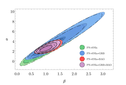
(a) Unified Model

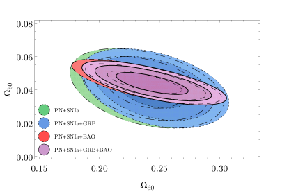
(b) $\Lambda$CDM

Figure 7: Confidence contours for the planes $(\beta,\alpha)$ of the UM (Fig. 7a) and $(\Omega_{d0},\Omega_{b0})$ of $\Lambda$CDM model (Fig. 7b) for various sets of data. The double-parameter estimates are little affected by the inclusion of GRB data in the case of both models: the $3\sigma$-confidence region of the set (PN + SNIa + GRB) is slightly smaller than the one for the set (PN + SNIa). Conversely, the confidence regions of the two-parameter estimates are considerably reduced by the inclusion of the BAO peaks in the statistical treatment.

Fig. 7 shows the confidence regions of the plane of parameters for the UM and $\Lambda$CDM model built with all data sets (SNIa + PN + GRB + BAO). It simultaneously displays the confidence contours of the previous analyses in order to indicate the impact of the different data set in constraining the domain value of the parameters.

Assuming that the set (PN + SNIa + GRB + BAO) gives the most realistic values for the cosmological parameters, we use the best-fit results for $\alpha$ and $\beta$ in Eq. (3) in order to obtain $w_{\text{U}}=w_{\text{dark}}$ of the dark sector of the universe according to UM. We also obtain $w_{\text{dark}}$ of the dark components in the $\Lambda$CDM model, using $\Omega_{d0}=0.24$ e $\Omega_{b0}=0.04$, for comparison. Both models are characterized by $w_{\text{dark}}(z)$ whose behavior are shown in Fig 8a. In the distant future, one anticipates $a\rightarrow\infty$, which implies $z\rightarrow-1$. The $\Lambda$CDM model gives $w_{\text{dark}}\left(z=-1\right)=-1$ while the UM leads to $w_{\text{dark}}\left(z=-1\right)=-0.90$. Notice that there are no big differences between the models in the region of small redshifts ($0\lesssim z\lesssim 0.5$). In addition, the present-day values ($z=0$) are $w_{\text{dark},0}=-0.75$ for the $\Lambda$CDM model and $w_{\text{dark},0}=-0.74$ for the UM. The functions $w_{\text{dark}}\left(z\right)$ of both models are equal in the region of $z\approx 2.5$ and slightly different elsewhere. Fig. 8b shows that the transition rates $dw_{\text{dark}}/dz$ for the two models are well distinguished. The peak of the transition rate for the $\Lambda$CDM model is $\left(dw_{\text{dark}}/dz\right)_{\max}=0.58$ and occurs at $z_{\max}=0.15$. For the UM we get $\left(dw_{\text{dark}}/dz\right)_{\max}=0.66$ at the larger redshift of $z_{\max}=0.44$. Both models interchange the quality of being the one with the larger transition rate depending on the value of $z$.

(a)

(b)

Figure 8: Comparison between fiducial $\Lambda$CDM model ($\Omega_{b0}=0.04$; $\Omega_{d0}=0.24$) and the unified model with the best-fit values of parameters $\alpha,$ $\beta$ and $\Omega_{b0}$ obtained with SNIa, GRB, BAO and PN data sets ($\alpha=2.4$; $\beta=0.99$; $\Omega_{b0}=0.041$). Plots of (a) $w_{\text{dark}}$ and (b) of $dw_{\text{dark}}/dz$  with respect to redshift for both models.

IV Final comments

This work presented a cosmological model unifying dark matter and dark energy through a parameterization in terms of the function $\arctan$. The three parameters of the model, $\alpha$, $\beta$ and $\Omega_{b0}$, were estimated admitting flat spacial curvature and using four observational data set, namely: PN, SNIa, GRB and BAO. The same combination of data was employed to constraint the $\Lambda$CDM model. This was used as standard with respect to which our model was compared.

The results were analyzed in two distinct ways: (i) the influence of the inclusion of GRB and BAO data in the estimates of the parameters of UM and $\Lambda$CDM model was discussed, and (ii) the direct comparison of UM and $\Lambda$CDM model was performed. In regard to point (i), it can be said that the inclusion of GRB data to the basic set (PN plus SNIa) does not modifies in a decisive way the confidence contours. In fact, there is a small difference between the curves in Fig. 7 even after increasing the number of GRB (by including 29 GRB to the set presented in Wei (2010)) and improving the interpolation technique of the calibration procedure. This indicates that, in spite of been promising as standard candles, GRB events are still not competitive in comparison to other sets of data such as the one for supernovae. Unlike the GRB data, the inclusion of BAO significantly restricts the parameter space; this is particularly true for the Unified Model (see Fig. 7a). With respect to point (ii), we can say that the UM and $\Lambda$CDM model exhibit statistically equivalent results for the baryon density $\Omega_{b0}$ and the redshift $z_{\text{eq}}$. Moreover, $\chi_{\text{red}}^{2}$ for both models are practically the same. In addition, the cosmic dynamics of the two models are very similar on the best-fit for all $z\geq 0$ (cf. Fig. 8a). The most pronounced difference between UM and $\Lambda$CDM occurs in their evolution toward the future, for $-1<z<0$. In fact, our parameterization leads to $\lim_{z\rightarrow-1}w_{\text{dark}}=-0.90$ and not to $\lim_{z\rightarrow-1}w_{\text{dark}}=-1$ as in the fiducial model. We can not affirm at the current stage of our investigation, if this difference between models is a physical effect due to the unification of the dark components in the UM or only an artifact of the parameterization for $w$ that we have chosen.

Future perspectives include two important subjects. The first concerns the dependence of the results on the specific parameterization for $w\left(z\right)$ chosen in our Unified Model. In particular, the $\arctan$ parameterization does not contain the $\Lambda$CDM model, i.e. there is no combination of the values of $\alpha$ and $\beta$ leading to the $w_{\text{dark}}$ of the $\Lambda$CDM model. This issue might be overcome by employing other parameterization such as one based on function $\tanh$. A second matter of investigation would be a possible UM-$\Lambda$CDM equivalence in a perturbative level. Indeed, could the statistical equivalence encountered in our data analysis (performed on the background) show up in a perturbative approach as well? These two question shall be addressed in further works.

Appendix A Akima’s interpolation method

Akima proposed in Akima (1970) a new interpolation technique aiming to overcome a difficulty shared by other interpolation methods, namely: the curve intercepting the data set does not present a natural evolution, as if it were drawn by hand. Typically, these other methods violate the continuity of the function or of its first-order derivative in some region of the domain; even if this flaw does not occur, the resulting curve presents undesirable oscillations or instabilities.

Ref. Akima (1970) establishes an interpolation method based in a piecewise function built with third-degree polynomials. The continuity of the composite function and its derivative are guaranteed by geometrical arguments. The slope $t$ of a given intermediate point among five neighboring points is calculated by

$$t=\dfrac{m_{2}\left|m_{4}-m_{3}\right|+m_{3}\left|m_{2}-m_{1}\right|}{\left|m_{4}-m_{3}\right|+\left|m_{2}-m_{1}\right|}~{},$$ (30)

where $m_{i}$ is the slope of the straight line connecting the $i$-th point (among the five points of the set) to the $\left(i+1\right)$-th point. For instance, $m_{2}$ is the angular coefficient of the straight line connecting the second and third points. The slopes uncertainties are obtained through the method of propagation of uncertainties after a long but straightforward calculation.

By using Eq. (30), one estimates the slopes for a set with $N$ points ($x_{i}$, $y_{i}$) except for the four points at the ends. Then, a third-degree polynomial is interpolated to the neighboring points respecting their coordinates and the determined slopes. Notice that by knowing the two coordinates and the two derivatives associated to a pair of points we are able to interpolate a third-degree polynomial, which has four degrees of freedom. However, we can not estimate the rate of change of the two last points at the ends using (30). These extremal points are interpolated to their internal neighbors, whose coordinates and slopes are known.

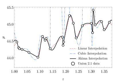
Figure 9: Comparison of the linear and cubic interpolation method with Akima’s technique. We use part of the Union2.1 data.

Fig. 9 shows part of the interpolation curves built according to linear, cubic and Akima’s interpolation methods. The zoom includes Union2.1 data from redshift $1$ to $1.4$. The linear interpolation produces a curve connecting the points in a direct form; but the first-order derivative of the function describing the curve is not continuous at the points.

On the other hand, cubic interpolation generates a smooth function with a continuous first-order derivative. However, huge instabilities and oscillations show up (such as those between point number 10 and point number 11 in the sample). This makes this method unsuited for the process of calibrating GRB curves.

For this end, Akima’s interpolation is the most adequate one because it gives a smooth and continuous function; this function has continuous derivative; and, the interpolated function follows the natural tendency of the points and in between them (i.e. there are no spurious oscillations).

Appendix B High-redshift GRB distance modulus

In subsection III.3, we have calibrated the $79$ high-redshift GRB compiled in Ref. Liu and Wei (2014). Here, the results are presented in Table LABEL:GRBTable.

Table 4: Distance modulus data for high-redshift supernovae.

z	$\mu$	$\sigma_{\mu}$
1.44	43.68	1.02
1.44	44.18	1.08
1.46	44.41	1.00
1.48	43.97	1.00
1.49	45.43	1.12
1.52	43.26	1.04
1.55	44.48	1.04
1.55	46.33	1.05
1.56	43.15	1.77
1.60	44.60	1.13
1.60	47.03	1.04
1.61	47.38	1.13
1.62	44.77	1.02
1.64	45.31	1.01
1.71	47.45	1.66
1.73	43.64	1.05
1.80	45.86	1.04
1.82	45.25	1.00
1.90	46.25	1.19
1.95	46.95	1.16
1.97	45.07	1.06
1.98	44.94	1.08
2.07	44.35	1.03
2.10	47.16	1.37
2.11	47.42	1.01
2.11	44.64	1.00
2.14	45.19	1.03
2.15	47.83	1.15
2.20	46.81	1.17
2.20	47.26	1.01
2.22	45.32	1.18
2.30	45.91	1.22
2.30	46.59	1.31
2.35	47.27	1.22
2.35	46.74	1.36
2.43	46.82	1.06
2.43	47.35	1.18
2.45	47.86	1.21
2.51	46.92	1.05
2.58	45.55	1.03
2.59	46.62	1.04
2.61	46.32	1.07
2.65	46.02	1.07
2.69	46.44	1.12
2.71	45.27	1.33
2.75	45.85	1.13
2.77	45.99	1.00
2.82	47.05	1.01
2.90	45.73	1.11
3.00	46.63	1.18
3.04	46.55	1.03
3.04	45.38	1.25
3.08	47.55	1.20
3.20	46.23	1.18
3.21	45.96	1.19
3.34	47.49	1.06
3.35	48.09	1.03
3.36	45.82	1.04
3.37	47.81	1.32
3.42	47.45	1.07
3.43	47.18	1.02
3.53	47.15	1.03
3.57	46.35	1.06
3.69	45.74	1.07
3.78	49.24	1.41
3.91	46.71	1.18
4.05	48.52	1.04
4.11	47.39	1.27
4.27	48.13	1.23
4.35	47.57	1.10
4.41	48.47	1.07
4.50	46.55	1.29
4.90	47.43	1.25
5.11	48.67	1.07
5.30	47.89	1.05
5.60	48.45	1.02
6.29	50.02	1.20
6.70	50.27	1.39
8.10	49.75	1.29

References

- Riess et al. (1998) A. G. Riess, A. V. Filippenko, P. Challis, A. Clocchiatti, A. Diercks, P. M. Garnavich, R. L. Gilliland, C. J. Hogan, S. Jha, R. P. Kirshner, et al., Astron. J. 116, 1009 (1998), [arXiv:astro-ph/9805201].
- Perlmutter et al. (1999) S. Perlmutter, G. Aldering, G. Goldhaber, R. Knop, P. Nugent, P. Castro, S. Deustua, S. Fabbro, A. Goobar, D. Groom, et al., Astrophys. J. 517, 565 (1999), [arXiv:astro-ph/9812133].
- Weinberg et al. (2013) D. H. Weinberg, M. J. Mortonson, D. J. Eisenstein, C. Hirata, A. G. Riess, and E. Rozo, Phys. Rep. 530, 87 (2013), [ arXiv:1201.2434 [astro-ph.CO]].
- Abergel et al. (2014) A. Abergel et al. (Planck), Astron. Astrophys. 571, A11 (2014), arXiv:1312.1300 [astro-ph.GA] .
- Percival et al. (2010) W. J. Percival, B. A. Reid, D. J. Eisenstein, N. A. Bahcall, T. Budavari, J. A. Frieman, M. Fukugita, J. E. Gunn, Ž. Ivezić, G. R. Knapp, et al., Mon. Not. R. Astron. Soc. 401, 2148 (2010), [arXiv:0907.1660 [astro-ph.CO]].
- Anderson et al. (2014) L. Anderson, É. Aubourg, S. Bailey, F. Beutler, V. Bhardwaj, M. Blanton, A. S. Bolton, J. Brinkmann, J. R. Brownstein, A. Burden, et al., Monthly Notices of the Royal Astronomical Society 441, 24 (2014).
- Wei and Nan Zhang (2009) H. Wei and S. Nan Zhang, EPJ C 63, 139 (2009), [arXiv:0808.2240 [astro-ph]].
- Schaefer (2007) B. E. Schaefer, Astrophys. J. 660, 16 (2007), [arXiv:astro-ph/0612285].
- Amati et al. (2002) L. Amati, N. Masetti, M. Feroci, P. Soffitta, J. Heise, L. Piro, E. Costa, F. Frontera, A. Antonelli, E. Palazzi, et al., Astron. Astrophys. 390, 81 (2002), [arXiv:astro-ph/0205230].
- Ellis et al. (2012) G. Ellis, R. Maartens, and M. MacCallum, Relativistic Cosmology (Cambridge University Press, New York, USA, 2012).
- Tolman (1934) R. C. Tolman, Proc. Natl. Acad. Sci. U.S.A. 20, 169 (1934).
- Bondi (1947) H. Bondi, Mon. Not. R. Astron. Soc. 107, 410 (1947).
- Buchert (2000) T. Buchert, Gen. Relat. Gravit. 32, 105 (2000), [arXiv:gr-qc/9906015].
- Räsänen (2011) S. Räsänen, Class. Quantum Grav. 28, 164008 (2011), [arXiv:1102.0408 [astro-ph.CO]].
- Wiltshire (2007) D. L. Wiltshire, Phys. Rev. Lett. 99, 251101 (2007), [arXiv:0709.0732 [gr-qc]].
- (16) D. L. Wiltshire, In S. E. Perez Bergliaffa and M. Novello (eds), Proceedings of the 15th Brazilian School on Cosmology and Gravitation, (Cambridge Scientific Publishers, 2014), [arXiv:1311.3787 [astro-ph.CO]].
- Weinberg (2008) S. Weinberg, Cosmology (Oxford Univ. Press, 2008).
- Bertacca et al. (2010) D. Bertacca, N. Bartolo, and S. Matarrese, Adv. Astron. 2010, 904379 (2010), arXiv:1008.0614 [astro-ph.CO] .
- Peebles and Vilenkin (1999) P. Peebles and A. Vilenkin, Phys. Rev. D 59, 063505 (1999), [arXiv:astro-ph/9810509].
- Kamenshchik et al. (2001) A. Kamenshchik, U. Moschella, and V. Pasquier, Phys. Lett. B 511, 265 (2001), [arXiv:gr-qc/0103004].
- Bento et al. (2002) M. Bento, O. Bertolami, and A. Sen, Phys. Rev. D 66, 043507 (2002), [arXiv:gr-qc/0202064].
- Padmanabhan and Choudhury (2002) T. Padmanabhan and T. R. Choudhury, Phys. Rev. D 66, 081301 (2002), [arXiv:hep-th/0205055].
- Scherrer (2004) R. J. Scherrer, Phys. Rev. Lett. 93, 011301 (2004), [arXiv:astro-ph/0402316].
- Giannakis and Hu (2005) D. Giannakis and W. Hu, Phys. Rev. D 72, 063502 (2005), [arXiv:astro-ph/0501423].
- Bertacca et al. (2007) D. Bertacca, S. Matarrese, and M. Pietroni, Mod. Phys. Lett. A 22, 2893 (2007), [arXiv:astro-ph/0703259].
- Giannantonio and Melchiorri (2006) T. Giannantonio and A. Melchiorri, Class. Quantum Grav. 23, 4125 (2006), [arXiv:gr-qc/0606030].
- Santos et al. (2006) F. Santos, M. Bedran, and V. Soares, Phys. Letters B 636, 86 (2006).
- Radicella and Pavón (2014) N. Radicella and D. Pavón, Physical Review D 89, 067302 (2014), [arXiv:1403.2601 [gr-qc]].
- Sharif et al. (2012) M. Sharif, K. Yesmakhanova, S. Rani, and R. Myrzakulov, European Physical Journal C-Particles and Fields 72, 1 (2012), [arXiv:1204.2181 [physics.gen-ph]].
- Makler et al. (2003a) M. Makler, S. Q. de Oliveira, and I. Waga, Physical Review D 68, 123521 (2003a), [arXiv:astro-ph/0306507].
- Makler et al. (2003b) M. Makler, S. Q. de Oliveira, and I. Waga, Physics Letters B 555, 1 (2003b), [arXiv:astro-ph/0209486].
- Alcaniz et al. (2003) J. Alcaniz, D. Jain, and A. Dev, Physical Review D 67, 043514 (2003), [arXiv:astro-ph/0210476].
- Balbi et al. (2007) A. Balbi, M. Bruni, and C. Quercellini, Physical Review D 76, 103519 (2007), [arXiv:astro-ph/0702423].
- Pietrobon et al. (2008) D. Pietrobon, A. Balbi, M. Bruni, and C. Quercellini, Physical Review D 78, 083510 (2008), [arXiv:0807.5077 [astro-ph]].
- Ishida et al. (2008) É. E. Ishida, R. R. Reis, A. V. Toribio, and I. Waga, Astropart. Phys. 28, 547 (2008), [arXiv:0706.0546 [astro-ph]].
- Giostri et al. (2012) R. Giostri, M. V. dos Santos, I. Waga, R. Reis, M. Calvao, and B. Lago, J. Cosmol. Astropart. Phys. 2012, 027 (2012), [arXiv:1203.3213[astro-ph.CO]].
- Fabris et al. (2011) J. C. Fabris, P. L. de Oliveira, and H. Velten, The European Physical Journal C 71, 1 (2011), [arXiv:1106.0645 [astro-ph.CO]].
- Wang et al. (2013) Y. Wang, D. Wands, L. Xu, J. De-Santiago, and A. Hojjati, Physical Review D 87, 083503 (2013), [arXiv:1301.5315 [astro-ph.CO]].
- Suzuki et al. (2012) N. Suzuki, D. Rubin, C. Lidman, G. Aldering, R. Amanullah, K. Barbary, L. Barrientos, J. Botyanszki, M. Brodwin, N. Connolly, et al., Astrophys. J. 746, 85 (2012), [arXiv:1105.3470 [astro-ph.CO]].
- Liu and Wei (2014) J. Liu and H. Wei, (2014), arXiv:1410.3960 [astro-ph.CO] .
- Wei (2010) H. Wei, J. Cosmol. Astropart. Phys. 2010, 020 (2010), [arXiv:1004.4951 [astro-ph.CO]].
- Akima (1970) H. Akima, J. ACM 17, 589 (1970).
- Bruni et al. (2013) M. Bruni, R. Lazkoz, and A. Rozas-Fernández, Mon. Not. R. Astronom. Soc. 431, 2907 (2013), [arXiv:1210.1880] [astro-ph.CO].
- Kirkman et al. (2003) D. Kirkman, D. Tytler, N. Suzuki, J. M. O’Meara, and D. Lubin, Astrophys. J. Suppl. Ser. 149, 1 (2003), [arXiv:astro-ph/0302006].
- Pettini and Cooke (2012) M. Pettini and R. Cooke, Mon. Not. R. Astron. Soc. 425, 2477 (2012), [arXiv:1205.3785 [astro-ph.CO]].
- O’meara et al. (2006) J. M. O’meara, S. Burles, J. X. Prochaska, G. E. Prochter, R. A. Bernstein, and K. M. Burgess, Astrophys. J. Lett. 649, L61 (2006), [arXiv:astro-ph/0608302].
- Adams (1976) T. F. Adams, Astron. Astrophys. 50, 461 (1976).
- Tytler et al. (1996) D. Tytler, X.-m. Fan, and S. Burles, Nature 381, 207 (1996), [arXiv:astro-ph/9603069].
- (49) S. Burles and D. Tytler, In A. Mezzacappa (ed), Proceedings of the Second Oak Ridge Symposium on Atomic & Nuclear Astrophysics, (Institute of Physics, Bristol,1998), [arXiv:astro-ph/9803071].
- O’meara et al. (2001) J. M. O’meara, D. Tytler, D. Kirkman, N. Suzuki, J. X. Prochaska, D. Lubin, and A. M. Wolfe, Astrophys. J. 552, 718 (2001), [arXiv:astro-ph/0011179].
- Pettini et al. (2008) M. Pettini, B. J. Zych, M. T. Murphy, A. Lewis, and C. C. Steidel, Mon. Not. R. Astron. Soc. 391, 1499 (2008), [arXiv:0805.0594 [astro-ph]].
- Riess et al. (2011) A. G. Riess, L. Macri, S. Casertano, H. Lampeitl, H. C. Ferguson, A. V. Filippenko, S. W. Jha, W. Li, and R. Chornock, Astrophys. J. 730, 119 (2011), [arXiv:1103.2976 [astro-ph.CO]].
- Freedman et al. (2012) W. L. Freedman, B. F. Madore, V. Scowcroft, C. Burns, A. Monson, S. E. Persson, M. Seibert, and J. Rigby, Astrophys. J. 758, 24 (2012), [arXiv:1208.3281 [astro-ph.CO]].
- Amendola et al. (2007) L. Amendola, G. C. Campos, and R. Rosenfeld, Phys. Rev. D 75, 083506 (2007), [arXiv:astro-ph/0610806].
- Goliath et al. (2001) M. Goliath, A. Goobar, R. Pain, R. Amanullah, and P. Astier, Astron. Astrophys. 380, 6 (2001), [arXiv:astro-ph/0104009].
- Riess et al. (2001) A. G. Riess et al. (Supernova Search Team), Astrophys. J. 560, 49 (2001), arXiv:astro-ph/0104455 [astro-ph] .
- Hu et al. (1995) W. Hu, D. Scott, N. Sugiyama, and M. White, Phys. Rev. D 52, 5498 (1995), [arXiv:astro-ph/9505043].
- Bromm and Loeb (2002) V. Bromm and A. Loeb, Astrophys. J. 575, 111 (2002), [arXiv:astro-ph/0201400].
- Li et al. (2011) M. Li, X.-D. Li, S. Wang, and Y. Wang, Commun. Theor. Phys. 56, 525 (2011), arXiv:1103.5870 [astro-ph.CO] .
- Ghirlanda et al. (2004a) G. Ghirlanda, G. Ghisellini, and D. Lazzati, Astrophys. J. 616, 331 (2004a), [arXiv:astro-ph/0405602].
- Liang and Zhang (2005) E. Liang and B. Zhang, Astrophys. J. 633, 611 (2005), [arXiv:astro-ph/0504404].
- Firmani et al. (2005) C. Firmani, G. Ghisellini, G. Ghirlanda, and V. Avila-Reese, Mon. Not. R. Astron. Soc.: Letters 360, L1 (2005), [arXiv:astro-ph/0501395].
- Graziani (2011) C. Graziani, New Astron. 16, 57 (2011), [arXiv:1002.3434 [astro-ph.CO]].
- Wang (2008) Y. Wang, Phys. Rev. D 78, 123532 (2008), [arXiv:0809.0657 [astro-ph]].
- Ghirlanda et al. (2004b) G. Ghirlanda, G. Ghisellini, D. Lazzati, and C. Firmani, Astrophys. J. Letters 613, L13 (2004b), [arXiv:astro-ph/0408350].
- Ghirlanda et al. (2006) G. Ghirlanda, G. Ghisellini, and C. Firmani, New J. Phys. 8, 123 (2006), [arXiv:astro-ph/0610248].
- Li et al. (2008) H. Li, J.-Q. Xia, J. Liu, G.-B. Zhao, Z.-H. Fan, and X. Zhang, Astrophys. J. 680, 92 (2008), [arXiv:0711.1792[astro-ph]].
- Liang and Zhang (2006) E. Liang and B. Zhang, Mon. Not. R. Astron. Soc.: Letters 369, L37 (2006), [arXiv:astro-ph/0512177].
- Liang et al. (2008) N. Liang, W. K. Xiao, Y. Liu, and S. N. Zhang, Astrophys. J. 685, 354 (2008), [arXiv:0802.4262[astro-ph]].
- Isobe et al. (1990) T. Isobe, E. D. Feigelson, M. G. Akritas, and G. J. Babu, Astrophys. J. 364, 104 (1990).
- Hu and Sugiyama (1996) W. Hu and N. Sugiyama, Astrophys. J. 471, 542 (1996).
- Albrecht et al. (2006) A. Albrecht et al., (2006), arXiv:astro-ph/0609591 [astro-ph] .
- Komatsu et al. (2009) E. Komatsu, J. Dunkley, M. Nolta, C. Bennett, B. Gold, G. Hinshaw, N. Jarosik, D. Larson, M. Limon, L. Page, et al., Astrophys. J. Suppl. Ser. 180, 330 (2009), [arXiv:0803.0547 [astro-ph]].
- Ichikawa et al. (2008) K. Ichikawa, T. Sekiguchi, and T. Takahashi, Phys. Rev. D 78, 083526 (2008), [arXiv:0803.0889 [astro-ph]].
- Olive et al. (2014) K. Olive, P. D. Group, et al., Chin. Phys. C 38, 090001 (2014).
- Farooq (2013) M. O. Farooq, Observational constraints on dark energy cosmological model parameters, Ph.D. thesis, Kansas State University, Manhattan, USA (2013).
- Beutler et al. (2011) F. Beutler, C. Blake, M. Colless, D. H. Jones, L. Staveley-Smith, L. Campbell, Q. Parker, W. Saunders, and F. Watson, Mon. Not. R. Astron. Soc. 416, 3017 (2011), [arXiv:1106.3366 [astro-ph.CO]].
- Watt and Thorne (2012) G. Watt and R. Thorne, J. High Energy Phys 2012, 1 (2012), [arXiv:1205.4024[hep-ph]].