Landau level spectroscopy of electron-electron interactions in graphene

Abstract

We present magneto-Raman scattering studies of electronic inter Landau level excitations in quasi-neutral graphene samples with different strengths of Coulomb interaction. The band velocity associated with these excitations is found to depend on the dielectric environment, on the index of Landau level involved, and to vary as a function of the magnetic field. This contradicts the single-particle picture of non-interacting massless Dirac electrons, but is accounted for by theory when the effect of electron-electron interaction is taken into account. Raman active, zero-momentum inter Landau level excitations in graphene are sensitive to electron-electron interactions due to the non-applicability of the Kohn theorem in this system, with a clearly non-parabolic dispersion relation.

Single-particle electronic states in graphene ostentatiously follow the dispersion of massless fermions, described by the Weyl equation in which the speed of light $c$ is simply scaled down to the band velocity $v\sim c/300$. Recently, however, more and more attention is paid to the effects of interactions and, in particular, to a modification of the dispersion relations and excitation spectra of quasi-particles induced by electron-electron interactions Elias et al. (2011); Chen et al. (2014); Basov et al. (2014). Indeed, graphene, and in particular pristine graphene, can hardly be considered as a weakly interacting system González et al. (1993); Hofmann et al. (2014); Kotov et al. (2012). The dimensionless interaction strength (the ratio between typical Coulomb and kinetic energies), which is rather small in genuine systems of quantum electrodynamics, $\alpha\approx{1}/137$ (the fine-structure constant), appears to be sizable in graphene, $(c/v)\alpha\approx{2}$. Screening (by a dielectric and/or conducting environment) naturally alters the strength of the electron-electron interaction in graphene, depending on its actual surrounding (substrate) and/or on the degree of departure from charge neutrality (electron/hole concentration). In a uniform dielectric environment characterized by a dielectric constant $\varepsilon$, the effective fine-structure constant is $\alpha_{\varepsilon}=(c/v)(\alpha/\varepsilon)$. The renormalization of graphene bands by electron-electron interactions has been mostly studied in the absence of magnetic fields Basov et al. (2014), whereas the anticipated effects Iyengar et al. (2007); Bychkov and Martinez (2008); Lozovik and Sokolik (2012); Shizuya (2010); Orlita and Potemski (2010) of these interactions in the regime of Landau quantized energy levels have been little explored so far Jiang et al. (2007); Chen et al. (2014).

In the present work, we investigate the effects of electron-electron interactions in graphene subjected to quantizing magnetic fields by probing its inter-Landau-level excitations with magneto-Raman scattering experiments Faugeras et al. (2011); Berciaud et al. (2014). We have studied three graphene systems with different dielectric environments. The non-interacting Dirac-like description of electronic states fails to account for the full set of our experimental observations. The velocity parameter, which we associate with each LL transition, is not a single value, but: (i) changes with the effective dielectric constant expected in our samples; the departure from the non-interacting picture is most pronounced for suspended graphene, weaker for graphene encapsulated in hexagonal boron nitride and rather small for graphene on graphite, (ii) varies logarithmically with the magnetic field, (iii) is higher for transitions involving higher LLs. These observations can be qualitatively described in the Hartree-Fock approximation Iyengar et al. (2007); Bychkov and Martinez (2008); Lozovik and Sokolik (2012) or by the first-order perturbation theory (FOPT) in $\alpha_{\varepsilon}$ González et al. (1993); Shizuya (2010). In particular, these calculations yield no full cancellation between vertex and self-energy corrections, implying violation of the Kohn theorem Kohn (1961) for the Dirac spectrum. Notably, the vertex corrections invert the tendency of lowering the electron velocity with energy, resulting from the self-energy terms, which accounts for feature (iii); see also  Jiang et al. (2007); Chen et al. (2014). However, FOPT fails on the quantitative level when $\alpha_{\varepsilon}$ is not small. Beyond FOPT, the leading terms in $\ln(B)$ can be addressed by the random-phase approximation (RPA)  González et al. (1999) (see also  Hofmann et al. (2014)), which turns out to match the experimental results quite well . Under some additional assumptions, we estimate two relevant parameters, the band width and bare band velocity, which define the renormalized electronic dispersion.

Conventional absorption spectroscopy of inter-LL transitions in graphene Orlita and Potemski (2010) is restricted to far-infrared spectral range ($\lambda\sim 100\>\mu\mbox{m}$) and does not offer the necessary spatial resolution, otherwise required for probing small graphene flakes. Better resolution is offered by visible light techniques, such as Raman scattering which is our method of choice. The possibility of observing Raman scattering from purely electronic, inter LL excitations Kashuba and Fal’ko (2009); Faugeras et al. (2011); Berciaud et al. (2014) is a recent addition to the wide use of Raman scattering spectra of phonons for the characterization of different graphene structures Ferrari and Basko (2013); Malard et al. (2009). We studied three distinct graphene systems: suspended graphene (G-S), graphene encapsulated in hexagonal boron nitride (G-BN) and graphene on graphite (G-Gr). G-S was suspended over a circular pit ($8\>\mu\mbox{m}$ in diameter) patterned on the surface of an Si/SiO₂ substrate (see Ref. Berciaud et al. (2009, 2014) for details of sample preparation). The G-BN structure consists of a graphene flake transferred onto a $\sim 50$ nm thick layer of hBN and then covered by another hBN flake of the same thickness, all together placed on an Si/SiO₂ substrate (see Ref. Dean et al. (2010) for details on a similar structure). The G-Gr flake was identified on the surface of freshly exfoliated natural graphite via mapping the Raman scattering response at a fixed magnetic field and searching for the position with the spectral features characteristic for graphene(see Ref. Faugeras et al. (2014) for details of the procedure). The experimental arrangements (see also Ref. Faugeras et al. (2011); Berciaud et al. (2014)) permitted Raman scattering experiments in magnetic fields up to $14$ T (supplied by a superconducting coil, data collected for G-BN) or up to $29/30$ T (supplied by a resistive magnet, data collected for G-S and G-Gr), at low temperatures ($4$ K) and with a spatial resolution of $\sim 1\>\mu\mbox{m}$ (diameter of the laser spot on the sample).

Magneto-Raman scattering spectra on G-Gr and G-S have been measured using the 514.5 nm line of an Ar⁺ laser for the excitation, in a simple, unpolarized light configuration. Experiments on G-BN were more demanding, due to a superfluous scattering/emission background originating from the hBN layers. To better resolve the electronic response from the G-BN species, laser excitation of a longer wavelength ($\sim 780$ nm) was chosen and the polarization resolved technique was implemented in the configuration of the circularly-polarized excitation beam and the back-scatted Raman signal, both of the same helicity Kühne et al. (2012); Kashuba and Fal’ko (2009). All experiments were performed using a laser power of $\sim 1$ mW at the sample. The sample was mounted on an X-Y-Z micro-positioning stage, which enabled us to map the Raman scattering response over the sample surface and to locate the graphene flake. The performance of our set-up is limited to the detection of Raman scattering signals exceeding an energy of $\sim 400$ cm^-1 from the laser line, due to various, spectral blocking elements/filters incorporated in the system. The magneto-Raman spectra have been recorded one after another while slowly sweeping the magnetic field. Typically, each spectrum was accumulated over a time interval during which the magnetic field was changed by $\sim 0.1$ T. Though the adequate electrical characterization of the investigated samples was not possible, we assume here that all our three graphene flakes are not far from being neutral systems; this is supported by many other studies of similar structures Bolotin et al. (2008); Berciaud et al. (2009); Dean et al. (2010); Neugebauer et al. (2009).

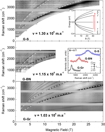
Figure 1: Gray scale map of the electronic response in the magneto-Raman scattering spectra response as a function of the magnetic field ($B$) for suspended graphene (G-S, top panel), graphene encapsulated in hBN (G-BN, middle panel) and graphene on graphite (G-Gr, bottom panel). Each map represents the collection of differential spectra (the $B=0$ spectrum has been subtracted from each spectrum measured in a magnetic field $B$). Dashed white lines account for the $B$-evolutions of two most pronounced inter LL excitations, expected within a single particle approach, when assuming a $B$-independent, but different for each sample, band velocity $v$. Upper inset: scheme of the Landau level fanchart in graphene; two, L_-1,1 and L_-2,2 inter Landau level excitations, well visible in the experiments on all samples, are indicated by red arrows. Middle panel inset: characteristic spectra due to $L_{-1,1}$ excitations measured at $B=8$ T for G-Gr (black symbols), G-BN (red symbols) and G-S (blue symbols). Gray curves are Lorentzian functions. Whitish horizontal ribbons on gray scale maps are to mask the (residual) contribution to Raman scattering due to phonons of graphene/graphite at $\sim 1600$ and $\sim 2700$cm^-1 as well as of Si substrate ( $\sim 520$ and $\sim 1000$cm^-1 at of hBN at $\sim 1370$cm^-1.

Besides the well-known spectral peaks due to phonons Ferrari et al. (2006); Ferrari and Basko (2013); Malard et al. (2009), the magneto-Raman scattering spectra of each of our graphene samples shows other, well-resolved peaks due to electronic inter-LL excitations, whose energies depend distinctly on the magnetic field. Those features are central for the present work. A collection of the related experimental data is presented in Fig. 1. In the zero-order approximation (single particle approach), the electronic dispersion in graphene is conical, $E(k)=\pm{v}k$. When a magnetic field $B$ is applied perpendicularly to the graphene plane, the continuous energy spectrum transforms into a series of discrete Landau levels ($L_{\pm n}$) with energies $E_{\pm n}=\pm\sqrt{2n}\,\hbar v/l_{B}$ (here $n=0,1,2,\ldots$, and $l_{B}=\sqrt{\hbar/(eB)}$ is the magnetic length); see upper inset to Fig. 1. We limit our considerations to the so-called symmetric $L_{-n}\rightarrow L_{n}$ ($L_{-n,n}$) inter LL transitions, which are expected to dominate the electronic Raman scattering response of graphene Kashuba and Fal’ko (2009), and appear at energies $\hbar\omega_{-n,n}=2E_{n}$, approximately. Tracing the $\hbar\omega_{-n,n}(B)$ dependences on top of gray-scale maps presented in Fig. 1, we recognize two transitions in the spectra of both G-S and G-BN, $L_{-1,1}$ and $L_{-2,2}$. G-Gr shows much richer spectra: a larger number of symmetric $L_{-n,n}$ transitions (at least up to $n=5$) as well as other, asymmetric, $\Delta|n|=1$ transitions. These latter transitions were predicted to be weakly allowed Kashuba and Fal’ko (2009) but are nevertheless well seen in G-Gr. We believe that the electronic quality (mobility) is the crucial factor which influences the richness of electronic Raman spectra of graphene. Aiming at a systematic study of the spectra in different dielectric environments, we focus on the $L_{-1,1}$ and $L_{-2,2}$ which are clearly seen in all three cases. In all our samples, the $L_{-1,1}$ transition starts to be visible at magnetic fields as low as $\sim 2.5$ T, at energies $E_{ons}\sim 1000$ cm^-1. This observation defines the upper bound for the Fermi energy, $E_{F}<E_{ons}/2\simeq 60$ meV, and confirms a relatively low doping in the studied graphene structures.

From the inspection of the $\hbar\omega_{-n,n}(B)$ traces drawn in Fig. 1, we easily identify the measured transitions, but at the same time notice some inconsistencies. First of all, using such an approximate data modelling we are forced to use different velocities for each of our graphene samples: $v$ is set to $1.30\times 10^{6}$ m/s, $1.15\times 10^{6}$ m/s, and $1.03\times 10^{6}$ m/s for G-S, G-BN, and G-Gr, respectively. The effect of different mean velocities for each graphene specimen is directly visualized in the lower inset to Fig. 1: at fixed $B$ but for different samples the $L_{-1,1}$ transitions appear at clearly distinct energies. Moreover, the above $v$ parameters can only be considered as the mean velocity values, averaged over different transitions and over the range of magnetic fields applied: note e. g. rather pronounced deviations between the white traces and the central peak positions for G-S (top panel of Fig. 1).

Figure 2: Magnetic field dependence ($B_{0}=$ 1 T) of the velocities associated with L_-1,1 and L_-2,2 inter Landau level excitations shown with, correspondingly, open circles (solid lines) and open stars (dashed lines), as derived from the experiment (data modelling), for G-S, G-hBN and G-Gr specimens. Straight lines follow the Eq. (4), (see also Eq. (2), with $\varepsilon_{*}=3.9$, $7.0$, and $12$ for G-S, G-hBN and G-Gr species, and the corresponding values for $\varepsilon_{\delta v}=1.3$, $3.7$ and $12$

.

The shortcomings of the above data modelling are emphasized in Fig. 2, the central figure of this paper. Data points (symbols) in this figure represent the velocity parameter which we associate with each observed transition and at each value of the magnetic field applied: $v_{n}^{exp}=\omega_{-n,n}^{exp}l_{B}/\sqrt{8n}$, where $\hbar\omega_{-n,n}^{exp}$ are the measured transition energies (central positions of the Raman scattering peaks). In the non-interacting case, all these velocities should collapse onto one single value. The extracted velocities $v_{n}^{exp}$, for different $L_{-n,n}$ transitions and for our three graphene structures, are plotted in Fig. 2 as functions of $\ln(l_{B_{0}}/l_{B})=\ln\sqrt{B/B_{0}}$, where the reference value of the magnetic field has been arbitrarily set to $B_{0}=1$ T. Each set of $v_{n}^{exp}$ versus $\ln(l_{B_{0}}/l_{B})$ data can be fairly approximated by a linear function. The $v_{n}^{exp}$-traces are parallel within a given graphene structure but show different slopes for different samples. These features point towards the effects of renormalization of the electronic velocity and of energies of inter-LL transitions by the electron-electron interactions.

For neutral graphene at $B=0$, the FOPT in $\alpha_{\varepsilon}=(c/v_{0})(\alpha/\varepsilon)$ gives the correction to the velocity $v$ González et al. (1993),

$$\frac{v}{v_{0}}=1-\frac{\alpha_{\varepsilon}}{4}\,\ln\frac{|E|}{W},\hskip 22.76228ptv=v_{0}-\frac{\alpha c}{4\varepsilon}\,\ln\frac{|E|}{W},$$ (1)

which depends on the electron energy $E$, counted from the Dirac point. Here $v_{0}$ is the bare velocity, and $W$ is the high-energy cutoff which is of the order of the electronic bandwidth (a few eV). The dielectric constant $\varepsilon$ can be taken as that of the surrounding medium for the suspended and encapsulated graphene In a finite magnetic field, the FOPT calculation of the correction to the transition energy $\hbar\omega_{-n,n}$, performed analogously to Ref. Shizuya (2010), gives the following correction to the velocity (see Supplementary Information for details):

$$v_{n}\equiv\frac{\omega_{-n,n}l_{B}}{\sqrt{8n}}=v_{0}+\frac{\alpha c}{4\varepsilon}(\mathcal{L}-\ln\frac{l_{B_{0}}}{l_{B}})+\frac{\alpha c}{4\varepsilon}C_{n}\hskip 14.22636pt$$ (2)

where $\mathcal{L}=\ln(Wl_{B_{0}}/\hbar{v}_{0})$ is a constant resulting from our choice of $l_{B_{0}}$ to set the horizontal scale in Fig. 2, and the numerical coefficients are $C_{1}=-0.398$ and $C_{2}=-0.197$. Note that the coefficient in front of the logarithm (which determines the slopes in Fig. 2) is the same in Eqs. (1) and (2). This is due to the fact that the leading logarithmic term in Eq. (2) can be obtained by simply replacing $E$ in Eq. (1) by the bare LL energy $E_{n}^{0}=\sqrt{2n}\,\hbar{v}_{0}/l_{B}$. On the other hand, the coefficients $C_{n}$ include both self-energy and vertex corrections, and have to be calculated explicitly.

Eq. (2) accounts qualitatively for the main experimental trends seen in Fig. 2. For each sample ($\varepsilon$), the dependences of $v_{n}^{exp}$ versus $\ln(l_{B_{0}}/l_{B})$ represent a set of parallel lines. The slope of these lines ($\propto 1/\varepsilon$ according to Eq. (2)) correlates with the expected, progressive increase of screening when shifting from G-S ($\varepsilon=1$) to G-BN ($\varepsilon_{\mathrm{hBN}}\approx{5}$), and to G-Gr, where the Coulomb interaction is screened by the conducting substrate, which can be viewed as a large effective $\varepsilon$. Notably, Eq. (2) also predicts $v_{2}>v_{1}$ for the same values of $\varepsilon$ and $B$ (as $C_{2}>C_{1}$), which would be the opposite if one simply substituted $E\to{E}_{n}^{0}$ in Eq. (1). This is due to vertex corrections. According to Eq. (2), $\delta{v}_{21}\equiv v_{2}-v_{1}=(\alpha c/4\varepsilon)(C_{2}-C_{1})$, which also agrees with the trend seen in Fig. 2, the decrease of $\delta{v}_{21}^{exp}$ with increasing $\varepsilon$.

However, Eqs. (1), (2) fail to reproduce quantitatively the data shown in Fig. 2. This is with regard to both the apparent amplitude of the slopes of $v_{n}^{exp}\propto\ln(B)$ dependences as well as the observed values of the relative shift $\delta{v}_{21}^{exp}$ between the velocities associated with $L_{1}$ and $L_{2}$ Landau levels.

If one uses Eq. (2) with some adjustable $\varepsilon_{*}$ (effective dielectric constant) instead of $\varepsilon$, the slopes in Fig. 2 would correspond respectively to $\varepsilon_{*}=3.9\pm 0.3$, $7.0\pm 0.5$ and $12.0\pm 1.0$ for G-S, G-BN and G-Gr, quite different from the known $\varepsilon=1$ and $\varepsilon=5$ for G-S and G-BN. This is not very surprising as the perturbative Eq. (2) does not have to work when the expansion parameter $\alpha_{\varepsilon}$ (exceeding 2 for $\varepsilon=1$) is not small. Fortunately, graphene offers another expansion parameter which can control the perturbation theory even when $\alpha_{\varepsilon}\sim{1}$. This parameter is identified as $1/N$, where $N$ is the number of electronic species: $N=4$ for graphene (the combined spin and valley degeneracy). In the $1/N$ expansion, an infinite number of terms of the perturbation theory is re-summed to all orders in $\alpha_{\varepsilon}$, selecting only those corresponding to the leading order in $1/N$ González et al. (1999). The resulting series is equivalent to RPA, and it was explicitly shown that the subleading contribution is indeed small Hofmann et al. (2014). The $1/N$ expansion has also been successfully used to describe the Coulomb renormalization of the electron-phonon coupling constants Basko and Aleiner (2008).

For the velocity renormalization at $B=0$, the $1/N$ expansion boils down to the modification (depending on $\alpha$) of the coefficient in front of the logarithm in Eq. (1) González et al. (1999). For moderate values of $\alpha<2.5$, typical for graphene, this modified coefficient can be well approximated (with 1% precision) by :

$$\frac{v_{0}\alpha_{\varepsilon}}{4}\to\frac{v_{0}\alpha_{\varepsilon}}{4(1+1.28\alpha_{\varepsilon})}=\frac{\alpha c}{4(\varepsilon+1.28\alpha c/v_{0})}$$ (3)

The above result can be seen as the added screening capacity, $\varepsilon\to\varepsilon_{1/N}=\varepsilon+1.28\alpha c/v_{0}$, by the graphene Dirac electrons themselves. Assuming $v_{0}=0.88\times 10^{6}$ m/s (see below), we obtain $\varepsilon_{1/N}=4.16$ for $\varepsilon=1$ (G-S) and 8.16 for $\varepsilon=5$ (G-BN), which are quite close to the measured values of $\varepsilon_{*}$. Obviously, it is hard to reason in terms of dielectric screening in case of G-Gr: a large $\varepsilon_{*}=12$ ($\varepsilon_{1/N}\simeq\varepsilon$) found for this graphene species must effectively account for efficient screening by the conducting graphite substrate.

At this point we apprehend the slopes of the lines in Fig. 2. The apparent amplitude of the velocity shifts $\delta{v}_{21}^{exp}$ remains to be analyzed. The measured values are $\delta{v}_{21}^{exp}\simeq\{0.084,0.039\}\times{10}^{6}$ m/s for G-S and G-BN, respectively, and we estimate that $\delta{v}_{21}^{exp}\leq 0.01\times{10}^{6}$ for G-Gr. On the other hand, Eq. (2) gives $\delta v_{21}=(\alpha c/4\varepsilon)(C_{2}-C_{1})=\{0.110,0.022,0.009\}\times{10}^{6}$ m/s for $\varepsilon=1$, $5$ and $12$, respectively, for G-S, G-BN and G-Gr. The replacement $\varepsilon\to\varepsilon_{1/N}$ in Eq. (2) results in an even worse agreement with the experiment. Indeed, this replacement is valid only for the leading logarithmic term, while the sub-logarithmic terms should be calculated explicitly, and the simple combination $C_{n}/\varepsilon$ will be replaced, generally speaking, by some more complicated one. Such a calculation has not been performed, to the best of our knowledge, and is beyond the scope of the present paper.

In order to describe the whole set of experimental data, we assume the following ansatz:

$$v_{n}=v_{0}+\frac{\alpha c}{4\varepsilon_{*}}(\mathcal{L}-\ln\frac{l_{B_{0}}}{l_{B}})+\frac{\alpha c}{4\varepsilon_{\delta v}}C_{n}$$ (4)

where $\varepsilon_{*}=3.9,\,7,\,12$ at the leading logarithmic term is in reasonable agreement with the $1/N$ expansion. In the sub-logarithmic term we fixed $C_{n}$ to be the same as in Eq. (2) and $\varepsilon_{\delta{v}}$ to depend only on $\varepsilon$ (but not on $n$). We do not have a proper theoretical justification for this assumption but adopting it, and setting $\varepsilon_{\delta{v}}=1.3,\,3.7,\,12$ in order to reproduce the experimentally observed $\delta{v}_{21}$, we are left with only two adjustable parameters, $v_{0}$ and $\mathcal{L}$. Their best matching values are $v_{0}=0.88\times{10}^{6}\>\mbox{m/s}$ and $\mathcal{L}=4.9$, that is, $W=(\hbar{v}_{0}/l_{B_{0}})^{\mathcal{L}}=3.1\>\mbox{eV}$, in fair agreement with the bare velocity and the characteristic bandwidth expected in graphene Gillen and Robertson (2010).

Concluding, using micro-magneto-Raman scattering spectroscopy, we have studied inter Landau level excitations in graphene structures, embedded in different dielectric environments. Understanding the energies of inter LL excitations clearly falls beyond the single particle approach (which refers to a simple Dirac equation) but appears to be sound when the effect of electron-electron interactions are taken into account. We confirm that the electronic properties of graphene on insulating substrates (weak dielectric screening) are strongly affected by electron-electron interactions, whereas conducting substrates favor the single particle behavior (graphene on graphite studied here, but likely also graphene on metals Kim et al. (2009); Coraux et al. (2008); Li et al. (2009) and graphene on SiC Sadowski et al. (2006); Orlita et al. (2008)). The present experiment together with the underlined theory show that the self-energy and vertex (excitonic) corrections to zero-momentum inter LL excitations do not cancel each other (breaking of the Kohn theorem), as often speculated in the literature Orlita and Potemski (2010) and already invoked in one of the early magneto-spectroscopy studies of graphene Jiang et al. (2007).

Here we evaluate the first-order correction to the energy $\hbar\omega_{-n,n}$ of the $L_{-1,1}$ inter-Landau-level electronic excitation due to the unscreened Coulomb interaction with the potential

$$U_{\mathbf{q}}=\frac{e^{2}}{\varepsilon}\,\frac{2\pi}{|\mathbf{q}|}\,(1-\delta_{\mathbf{q},0}),$$ (5)

where $e$ is the electron charge, $\varepsilon$ is the background dielectric constant, $\mathbf{q}$ is the two-dimensional wave vector, and the last factor accounts for the neutralizing ionic background. The first-order correction is given by the expectation value of the interaction Hamiltonian in the state

$$|L_{-n,n}\rangle=\sum_{p_{x}}\sum_{v=K,K^{\prime}}\sum_{\sigma=\uparrow,\downarrow}\hat{c}^{\dagger}_{n,p_{x},v,\sigma}\hat{c}_{-n,p_{x},v,\sigma}|0\rangle,$$ (6)

where $\hat{c}^{\dagger}_{n,p_{x},v,\sigma}$ is the creation operator for an electron with the $x$ component of momentum $p_{x}$ (we use the Landau gauge) on the $n$th Landau level in the valley $v$ and with the spin projection $\sigma$. $|0\rangle$ is the ground state of the system, corresponding to all negative Landau levels filled, all positive Landau levels empty, and the level $n=0$ half-filled. This expectation value is given by

$$\hbar\omega_{-n,n}-\hbar\omega_{-n,n}^{0}=\Sigma_{n}-\Sigma_{-n}+V_{-n,n},$$ (7)

where $\Sigma_{\pm{n}}$ and $V_{-n,n}$ are the self-energy and vertex corrections, respectively, given by

$$\Sigma_{\pm{n}}=-\sum_{n^{\prime}}{f}_{n^{\prime}}\int\frac{d^{2}\mathbf{q}}{(2\pi)^{2}}\,\tilde{J}_{n^{\prime},\pm{n}}(-\mathbf{q})\,\tilde{J}_{\pm{n},n^{\prime}}(\mathbf{q})\,U_{\mathbf{q}},\quad$$ (8)

$$V_{-n,n}=-\int\frac{d^{2}\mathbf{q}}{(2\pi)^{2}}\,\tilde{J}_{n,n}(-\mathbf{q})\,\tilde{J}_{-n,-n}(\mathbf{q})\,U_{\mathbf{q}}.$$ (9)

Here $f_{n^{\prime}}$ is the average occupation of the level $n^{\prime}$ ($f_{n^{\prime}<0}=1$, $f_{0}=1/2$, and $f_{n^{\prime}>0}=0$), and

$$\tilde{J}_{n\neq{0},n^{\prime}\neq{0}}(\mathbf{q})=\frac{J_{|n|,|n^{\prime}|}(\mathbf{q})+\mathop{\rm sign}(nn^{\prime})\,J_{|n|-1,|n^{\prime}|-1}(\mathbf{q})}{2},$$

$$\tilde{J}_{n\neq{0},0}(\mathbf{q})=\frac{J_{|n|,0}(\mathbf{q})}{\sqrt{2}},\quad\tilde{J}_{0,n\neq{0}}(\mathbf{q})=\frac{J_{0,|n|}(\mathbf{q})}{\sqrt{2}},$$

$$\tilde{J}_{0,0}(\mathbf{q})=J_{0,0}(\mathbf{q}),$$

$$J_{n,n^{\prime}}(\mathbf{q})=(-1)^{n^{\prime}+\min\{n,n^{\prime}\}}\sqrt{\frac{\min\{n,n^{\prime}\}!}{\max\{n,n^{\prime}\}!}}\,e^{-q^{2}l_{B}^{2}/4}$$

$$\qquad\qquad{}\times\left(\frac{q_{x}+iq_{y}}{q}\right)^{n-n^{\prime}}\left(\frac{ql_{B}}{\sqrt{2}}\right)^{|n-n^{\prime}|}$$

$$\qquad\qquad{}\times\mathrm{L}_{\min\{n,n^{\prime}\}}^{(|n-n^{\prime}|)}(q^{2}l_{B}^{2}/2),$$

where

$$\mathrm{L}_{m}^{(\alpha)}(\xi)=\sum_{k=0}^{m}\frac{(-1)^{k}(m+\alpha)!}{k!\,(m-k)!\,(\alpha+k)!}\,\xi^{k}.$$

is the associated Laguerre polynomial.

The vertex correction is straightforwardly evaluated,

$$V_{-n,n}=-\frac{e^{2}}{4\varepsilon{l}_{B}}\int\limits_{0}^{\infty}\frac{d\xi\,e^{-\xi}}{\sqrt{2\xi}}\,\left[\mathrm{L}_{n}^{(0)}(\xi)+\mathrm{L}_{n-1}^{(0)}(\xi)\right]^{2},$$

which gives explicitly

$$\left\{V_{-1,1},\,V_{-2,2},\,V_{-3,3}\right\}=-\frac{e^{2}}{\varepsilon{l}_{B}}\,\sqrt{\frac{\pi}{2}}\left\{\frac{11}{16},\,\frac{145}{256},\,\frac{515}{1024}\right\}.$$ (10)

For the self-energies of the lowest Landau levels we obtain

$$\Sigma_{0}=-\frac{e^{2}}{\varepsilon{l}_{B}}\int\limits_{0}^{\infty}\frac{d\xi\,e^{-\xi}}{\sqrt{2\xi}}\left(f_{0}+\sum_{n=1}^{\infty}\frac{\xi^{n}}{2n!}\right)=-\frac{e^{2}}{\varepsilon{l}_{B}}\sqrt{\frac{\pi}{2}}\left[f_{0}+\frac{1}{2}\sum_{n=1}^{\infty}\frac{(2n)!}{4^{n}(n!)^{2}}\right],$$

$$\Sigma_{\pm{1}}=-\frac{e^{2}}{\varepsilon{l}_{B}}\sqrt{\frac{\pi}{2}}\left[\frac{f_{0}}{4}+\sum_{n=1}^{\infty}\frac{2n-1/4\mp\sqrt{n}}{4(n-1/2)}\,\frac{(2n)!}{4^{n}(n!)^{2}}\right],$$

$$\Sigma_{\pm{2}}=-\frac{e^{2}}{\varepsilon{l}_{B}}\sqrt{\frac{\pi}{2}}\left[\frac{3f_{0}}{16}+\frac{15\mp{4}\sqrt{2}}{64}\right.+$$

$$\hskip 28.45274pt+\left.\sum_{n=2}^{\infty}\frac{64n^{2}-88n+9\pm\sqrt{2n}(36-32n)}{128(n-1/2)(n-3/2)}\,\frac{(2n)!}{4^{n}(n!)^{2}}\right],$$

$$\Sigma_{\pm{3}}=-\frac{e^{2}}{\varepsilon{l}_{B}}\sqrt{\frac{\pi}{2}}\left[\frac{5f_{0}}{32}+\frac{199\mp{4}\sqrt{3}(4+5\sqrt{2})}{512}\right.+$$

$$\hskip 28.45274pt+\left.\sum_{n=3}^{\infty}\frac{256n^{3}-928n^{2}+816n-75\mp\sqrt{3n}(128n^{2}-416n+300)}{512(n-1/2)(n-3/2)(n-5/2)}\,\frac{(2n)!}{4^{n}(n!)^{2}}\right].$$

In each of the above expressions, the sum is divergent, so the upper limit should be set to some large $n_{max}$. Then, each $\Sigma_{\pm{n}}\propto{n}_{max}$. The energy differences diverge only logarithmically,

$$\Sigma_{\pm{1}}-\Sigma_{0}=\pm\frac{e^{2}}{\varepsilon{l}_{B}}\left(0.290240+\frac{1}{\sqrt{2}}\frac{\ln{n}_{max}}{4}\right),$$ (11)

$$\Sigma_{\pm{2}}-\Sigma_{0}=\pm\frac{e^{2}}{\varepsilon{l}_{B}}\left(0.256384+\frac{\ln{n}_{max}}{4}\right),$$ (12)

$$\Sigma_{\pm{3}}-\Sigma_{0}=\pm\frac{e^{2}}{\varepsilon{l}_{B}}\left(0.196799+\sqrt{\frac{3}{2}}\,\frac{\ln{n}_{max}}{4}\right),$$ (13)

where $f_{0}$ has been set to $1/2$. Relating $n_{max}$ to the energy cutoff $W$ as $\sqrt{2n_{max}}\,(\hbar{v}_{0}/l_{B})=W$, we arrive at Eq. (2) of the main text with $C_{1}=-0.398$, $C_{2}=-0.197$, $C_{3}=-0.193$.