Inference on the Network Evolution in BitTorrent Mainline DHT
Abstract
Network size is a fundamental statistic for a peer-to-peer system but is generally considered to contain too little information to be useful. However, most existing work only considers the metric by itself and does not explore what features could be extracted from this seemingly trivial metric. In this paper, we show that Fourier transform allows us to extract frequency features from such time series data, which can further be used to characterize user behaviors and detect system anomalies in a peer-to-peer system automatically without needing to resort to visual comparisons. By using the proposed algorithm, our system successfully discovers and clusters countries of similar user behavior and captures the anomalies like Sybil attacks and other real-world events with high accuracy. Our work in this paper highlights the usefulness of more advanced time series processing techniques in analyzing network measurements.
Keywords:
BitTorrent Mainline DHT, User behavior characterization, anomaly detection, Fourier transform, Feature extraction, Classification1 Introduction
Measuring the properties of a system can not only report various system statistics, but can also be used to expose underlying relationships between general system dynamics and other characteristics. This, however, requires that the measurements capture the essential characteristics or that appropriate processing is done to the measurements to enable extraction of useful features. In many existing measurement work, measured data is simply reported as-is, which makes obtaining deeper insight from the measurements difficult. While such “naive” results hold some interest in themselves, more advanced methods yield more insight and enable automatic comparison of many interesting features.
System measurement has its irreplaceable importance in the Peer-to-Peer (P2P) research. The purpose of the measurements is not merely meant to report the system statistics but also expected to expose the underlying relations between the system dynamics and other characteristics. However, such insight from the statistics can only be obtained given the data is properly processed, in other words, when the useful information is extracted. E.g. the network size is a fundamental statistic for a P2P system, and network evolution data describes how the size changes as a function of time. However, network size as a system metric is generally considered containing too little information to be useful. On the contrary, the fact is network evolution data contains much more useful and interesting information than most people expect. As we will show in this paper, such information can help us finding similar use patterns of different countries and even detecting system anomalies.
In this paper we use Fourier transform to extract representative features from a time series of measurements of the size of BitTorrent MLDHT network. Fourier transform is not sensitive to issues like temporal alignment of different samples and it provides us with an easy way of obtaining a “fingerprint” of the data sample. We apply this technique to measurements in different ways and show how it can be used to identify many relevant features of the network. Fourier transforms are a well-known and widely-used technique in other fields, but they have not so far been much used in network measurement work.
Specifically, our contributions are as follows:
-
1.
We use Fourier transforms to extract frequency-based features from network evolution data. The simple algorithm is also applicable to other time series data in P2P measurements.
-
2.
We show the frequency-based features are robust to the noisy data and can be used to characterize user behaviors and detect system anomalies. Our method indicates the data sets with simple structure may contain more information than we have expected.
-
3.
We implement our algorithm and evaluate it on a realistic monitoring system. We report its actual performance along with some interesting findings.
2 Background on Fourier Transform
The original idea of Fourier transform is to decompose a function111In this paper, we use function, signal and time series interchangeably as long as it does not cause ambiguity in the context. into a summation of a series of sinusoids waves, or in other words, projecting a function from one function base to another. Often, a discretized form consisting only of consecutive sampling points is used which leads to the discrete Fourier transform. In complex form, it can be written as follows:
| (1) | |||
| (2) |
where is the imaginary unit and denotes the Fourier coefficient of frequency in the complex form. Fourier transform in the complex plane is much simpler than the trigonometric form and can be efficiently calculated using Fast Fourier Transform (FFT). For a more thorough overview of Fourier transform and related techniques, please refer to [1, 2].
Despite of its wide application in many fields, Fourier transforms (or other similar methods) have not been commonly used in peer-to-peer research even though a lot of research has focused on collecting data [3, 4, 5, 6, 7, 8, 9]. The same is largely true of many other network measurement research. Though in many existing works, the focus is on different aspects of the system ranging from security and topology to economic incentives, the general methodology is in many cases similar in the sense that the goal is to find a pattern by extracting as much information as possible from time series data. For this kind of work, Fourier transforms and other mechanisms, such as wavelets, can provide interesting insight. In this paper we show that using Fourier transforms, we are able to extract meaningful insight from a simple time series of network size evolution data. Past works that have looked at this kind of data typically have been limited to describing quantitative numbers about the size evolution or usage in different countries. Our work shows that we can classify different countries according to their usage behavior and easily visualize how different countries group together. Naturally, more sophisticated methods, such as wavelets, could also be used and would likely yield additional insights; our goal in this paper is to highlight the benefits of using proper time series analysis techniques and open the road for further research.
3 Frequency-Based Feature
To compare user behavior and detect behavior changes, as well as to capture anomalies, we first need to identify a robust feature set. As mentioned, we apply Fourier transform to country-level network size evolution and then generate a frequency-based feature set as its unique “fingerprint”. In this section, we formulate the relevant definitions and detail the actual steps of feature extraction from network size evolution. Then we show how the similarities derived can be used to discover patterns and detect anomalies. Fig. 1 depicts the general workflow of the proposed method. Starting from the raw time series data, i.e., estimated number of users in a country or the whole system, we perform the Fourier transform to obtain the frequency domain features. Using singular value decomposition, we reduce the dimensionality of the feature vector to allow for easier comparison of different samples. Below we will detail these steps.
3.1 Feature Extraction with FFT
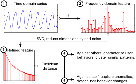
Our data sets are collected from a monitoring system similar to the one in [3], which continuously estimates the network size of MLDHT by crawling its ID space. Each crawl generates a full list of IP addresses in a subspace. Using the methodology presented in [3], we can get a good estimate of the total network size. System-level network evolution can be obtained by a series of such measurements, then further decomposed to country-level (even city-level) evolution based on their IP blocks. We use the MaxMind service222www.maxmind.com to perform the mapping of IP addresses to geographical locations.
Definition 1
Network evolution of a specific country is a time series which gives the network size of at time .
For simplicity of notation, we drop the subscript if it causes no confusion in the context. Our actual measurements show that is practically a stationary function with a period of one week for almost all the countries, because user behavior is generally different in the weekends than weekdays, but similar from one week to another. So in our calculation, we adopt a period window of seven consecutive days (irrelevant of the starting point) which consists of discretized sampling points , , … . Fourier transform of this time series gives another complex vector of the same length which we will use as the starting point of the frequency-based feature set.
Definition 2
Frequency-based feature set of a specific network evolution series is a real vector where element represents the normalized Fourier coefficient associated with frequency in .
Specifically,
| (3) |
where the normalizer equals
| (4) |
above denotes Euclidean norm. E.q.(3) is simply the Fourier coefficient of frequency normalized by . E.q.(4) calculates the length of the raw coefficient vector in -dimensional space which is used as an normalizer in (3). The purpose of normalization is to filter out the effect from the absolute network size but focusing on the pure pattern of a curve. Essentially, we are using a normalized vector of Fourier coefficients as the feature set, where each element represents the amplitude of its associated frequency component in the original signal .
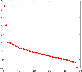
High dimensional features are usually noisy, redundant and expensive to compare. Common technique for dimensionality reduction is Singular Value Decomposition (SVD). Fig. 2a shows the semi-log plot of the singular values in a feature set. We can see the first two components dominate the system dynamics. More precisely, the first principal component itself captures over 77% of the energy. In practice, we only keep the first 40 principal components (denoted by ) in order to retain 99.20% of the system energy. The refined feature set can be calculated with as follows, and in our case.
| (5) |
The actual computation can be done efficiently since FFT and SVD are standard routines in scientific computing libraries. Once the feature set is successfully extracted, we can use it to characterize user behavior and further look for similar patterns with properly defined similarity metric as follows.
Definition 3
Similarity of two feature sets and is defined as their Euclidean distance in -dimensional space.
| (6) |
The code in Algorithm 1 shows how the features are actually extracted and pairwise similarity is calculated. The key input is a matrix where each column vector represents a country’s network evolution of a 7-day window. The column vector contains 2048 discretized sampling points. is the number of principal components we want to keep in the final feature set. The rest of the code is easy to understand. Lines 4 - 8 iterate all the countries, where line 5 calculates the Fourier coefficients using FFT, and line 6 normalizes it to a real unit vector. Note that in our case abs function translates each complex element in into corresponding amplitude. Lines 9 and 10 reduce the feature set dimensionality by taking the first principal components. Function pdist in line 11 calculates the pairwise distance for a given point set. Eventually, each column in the output matrix represents a -dimensional feature set of a country, and contains their pairwise similarity metrics.
3.2 Anomaly Detection Based on Fluctuation
In a broad sense, a system anomaly indicates a significant change in a certain system metric which is usually reflected as fluctuation or drift in the corresponding time series. Such anomalies might be due to service breakdowns, system attacks, or drastic changes in use pattern. Detecting such anomalies with satisfying sensitivity and fall-out rate is generally difficult, especially with noisy data.
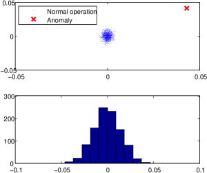
For an ideal stationary periodic signal, the feature set is time-invariant and remains constant since it has been projected to the frequency domain. Even in a practical setting where some noise is inevitable, the feature set does not vary much if the overall evolution remains constant. In other words, the feature set in each measurement should only fluctuate around its mean and at a very small scale. Fig. 2b plots the variation of system-level features with the mean subtracted from the values. The lower figure shows that the feature distribution during normal operations is very narrow and Gaussian-like. In the upper figure, we can see all the corresponding blue points scattered around the origin within a very small area. The big red cross in the top-right corner marks the deviant feature measured when a Sybil attack was launch in September 2011 [10]. We can see it deviates very far away from the center and this deviation can be used as an indicator of an anomaly. Note that this only indicates a possible anomaly but does not (necessarily) yield information about the nature of the anomaly.
Therefore, we can take advantage of the stability of the frequency-based feature and use it as an anomaly indicator. Technically, it is done by reusing the similarity metric introduced in Section 3.1 against a signal itself, namely .
Definition 4
Anomaly indicator for an entity is defined as , where and denote the current measurement on and its average value respectively.
By definition is the deviation of the current measured to its own average. In other words, it measures how similar a signal to itself on average in each measurement. In practice, sample mean is used in place of the true average. An alarm can be triggered if the deviation is large enough, e.g., and denotes the variance of . In the actual implementation, we incorporate supervised machine learning technique to achieve good balance between sensitivity and fall-out rate.
4 Evaluation in the Wild
In the following, we briefly report the performance of the proposed method on a realistic monitoring system with some selected results. We evaluate our method in terms of its effectiveness of clustering similar user behaviors and the accuracy of capturing anomalies. We extended the basic system proposed in [3] by incorporating the feature extraction and anomaly detection modules, and reimplemented it on Spark. The system is not only able to quickly respond to the continuous real-time samples, but also capable of fast processing terabytes historical archives.
4.1 Discover Similarity in Use Patterns
The evolution of network size represents how and when the system is accessed and used, which further reflects the characteristics of the use patterns from a group of geographically-close users. The frequency-based feature is expected to capture the similarity in such patterns and reflect in the proposed similarity metric defined in Section 3.1.
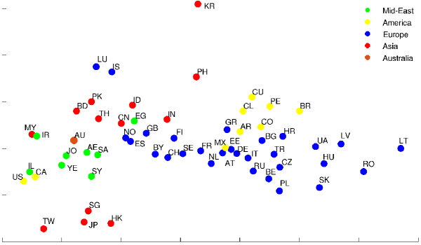
To gain an intuitive understanding of the effectiveness of such mechanisms, we use the first two principal components in the feature set and plot them in Fig.3a. Countries are marked with different colors according to their geographical regions, and their coordinates in the figure are determined by the two principal components. At the first glance, most of the countries gather together roughly based on their geographical proximity. This is understandable since the geographical closeness usually indicates that the countries share social, cultural, and economic bonds which lead to similar user behavior. For example, among the European countries, most East European countries stay at the right of the figure while the most Western ones gather in the middle.
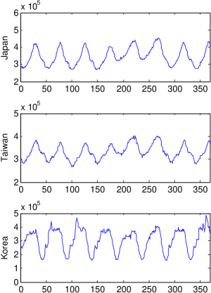
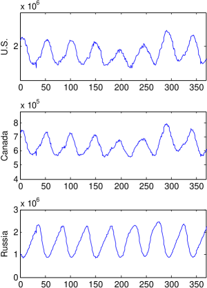
However, we can see some interesting phenomena among some sets of countries. Comparing Japan, Taiwan, and Korea, we see that Korea is mapped to a very different place in Figure 3a and if we compare the actual daily patterns of these three countries, as shown in Figure 3b, we see that the Korean pattern is clearly different from that of Japan or Taiwan. Similar observation holds when comparing Korea with Singapore or Hong Kong which map close to Japan and Taiwan in Figure 3a. Likewise, Figure 3c compares USA, Canada, and Russia, and the visual differences in the patterns are also reflected in the placement of the three countries in Figure 3a. (USA and Canada are towards the left, Russia is in the middle.)
We have compared other groupings of countries and have seen that countries that map close to each other in Figure 3a have visually similar daily patterns. However, data in Figure 3a only serves to classify countries into different groupings. The distances between different countries do not really serve as an indicator of how different their daily patterns are; instead it only indicates the existence of a difference.
4.2 Detecting Nontrivial Anomalies with Learning
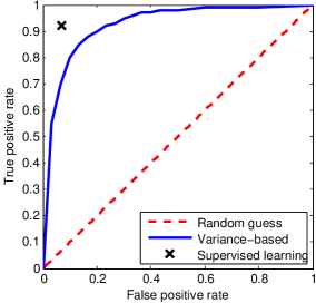
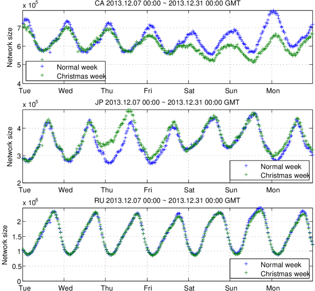
Despite different potential causes, the system anomalies are reflected as statistically significant changes in the feature by definition. Anomaly detection takes advantage of the stability of frequency-based features, and issues an alarm when the deviation is large enough. As we have introduced in Section 3.2, the threshold of triggering an alarm can either be manually set or automatically learnt from labelled data. The blue solid line in the Fig. 4a shows the performance by simply varying variance-based threshold in the ROC space. Recall that ROC curve shows the trade-off between sensitivity (true positive rate) and fall-out (false positive rate) in a classification system and increasing the threshold improves fall-out by sacrificing sensitivity. The red dashed line in Fig. 4a represents a pure guess, which serves as a baseline that any rational algorithm should be above and the top-left corner represents perfect accuracy. Our evaluation shows that simple variance-based threshold can already achieve good accuracy. In the actual system, we adopted an naive Bayesian classifier trained on a data set of 500 labelled anomalies, and its accuracy is plotted as a black cross in the same Fig. 4a. As we can see, frequency-based feature with basic supervised learning leads to a high-accuracy detection module.
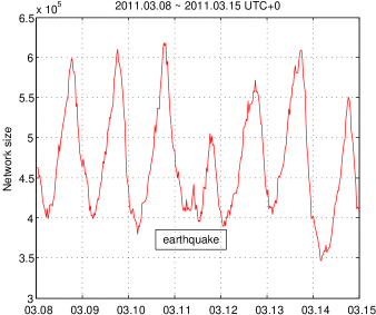
Besides the large-scale Sybil attack mentioned in Section 3.2 and many others, our anomaly detection system also successfully captured a lot of interesting real-world events. For example, there was a severe earthquake happened in Tōhoku, Japan on March 11th, 2011. Figure 4b shows the network evolution of the corresponding week. Our feature extraction method would have indicated an alarm due to the large-scale network breakdown which caused tens of thousands of computers disconnected from the network. While Figure 4b illustrates the impacts from natural causes, Figure 4c on the right shows how the social and cultural events can change user behaviors. Figure 4c plots the Christmas week in 2013 with green lines for Canada, Japan, and Russia (from top to bottom). To highlight the pattern drift, the network evolution of a normal week is also plotted in the same figure with blue line. Interestingly, we notice while there was significant drop in the network size during Christmas in Canada (actually in most western countries), this number increased quite a lot in Japan (also in many other Asian countries). Russia, on the other hand, did not change much during this time period. One possible explanation could be that in Russia Christmas is celebrated according to the Orthodox calendar, meaning that it falls a few weeks later than in Western countries; in other words, the week shown in Figure 4c is simply a normal week compared with another normal week.
4.3 Summary
As the results above show, the features extracted via Fourier transform allow us to look at the data from another point of view and observe different phenomena more easily. For example, characterizing the diurnal patterns in different countries is readily visible in Figure 3 without the need to compare every country pairs visually.
5 Conclusion
In this paper, we showed that Fourier transform can be used as a simple yet powerful tool to extract representative information from time series data in P2P measurements. Applying Fourier transform on network size evolution data, we showed that this seemingly trivial statistic contains rich information. The extracted frequency-based feature can be effectively used to characterize user behaviors and detect system anomalies. We implemented a monitoring system with the proposed algorithm and evaluated its actual performance in the realistic environment with many interesting real-world findings. Our algorithm successfully discovered nontrivial use patterns and captured anomalies with high accuracy. In the future, we plan to apply this technique on a broader range of data sets and also explore its other potential applications in P2P monitor and measurement research.
References
- [1] R. N. Bracewell, “Fourier transform and its applications,” 1980.
- [2] P. Bloomfield, Fourier analysis of time series: an introduction. John Wiley & Sons, 2004.
- [3] L. Wang and J. Kangasharju, “Measuring large-scale distributed systems: case of bittorrent mainline dht,” in Peer-to-Peer Computing (P2P), 2013 IEEE Thirteenth International Conference on, Sept 2013, pp. 1–10.
- [4] C. Decker, R. Eidenbenz, and R. Wattenhofer, “Exploring and improving bittorrent topologies,” in Peer-to-Peer Computing (P2P), 2013 IEEE Thirteenth International Conference on, Sept 2013, pp. 1–10.
- [5] R. Farahbakhsh, A. Cuevas, R. Cuevas, R. Rejaie, M. Kryczka, R. Gonzalez, and N. Crespi, “Investigating the reaction of bittorrent content publishers to antipiracy actions,” in Peer-to-Peer Computing (P2P), 2013 IEEE Thirteenth International Conference on, Sept 2013, pp. 1–10.
- [6] Z. Jelveh and K. Ross, “Profiting from filesharing: A measurement study of economic incentives in cyberlockers,” in Peer-to-Peer Computing (P2P), 2012 IEEE 12th International Conference on, Sept 2012, pp. 57–62.
- [7] J. Timpanaro, T. Cholez, I. Chrisment, and O. Festor, “Bittorrent’s mainline dht security assessment,” in New Technologies, Mobility and Security (NTMS), 2011 4th IFIP International Conference on, Feb 2011, pp. 1–5.
- [8] C. Zhang, P. Dhungel, D. Wu, and K. Ross, “Unraveling the bittorrent ecosystem,” Parallel and Distributed Systems, IEEE Transactions on, vol. 22, no. 7, pp. 1164–1177, July 2011.
- [9] G. Mega, A. Montresor, and G. Picco, “On churn and communication delays in social overlays,” in Peer-to-Peer Computing (P2P), 2012 IEEE 12th International Conference on, Sept 2012, pp. 214–224.
- [10] L. Wang and J. Kangasharju, “Real-world sybil attacks in BitTorrent Mainline DHT,” in Proceedings of IEEE Globecom, Dec. 2012.
Appendix
| BR | CA | CN | EG | FI | GB | HK | IL | IN | IT | JP | KR | NL | PL | RU | SE | US | |
|---|---|---|---|---|---|---|---|---|---|---|---|---|---|---|---|---|---|
| BR | 0.00 | 8.92 | 6.00 | 5.56 | 4.23 | 5.16 | 6.46 | 9.10 | 4.46 | 1.81 | 7.34 | 3.61 | 3.02 | 1.09 | 1.69 | 3.95 | 9.31 |
| CA | 8.92 | 0.00 | 2.95 | 3.39 | 4.69 | 3.77 | 2.59 | 0.19 | 4.48 | 7.16 | 1.72 | 5.78 | 5.92 | 8.22 | 7.33 | 4.97 | 0.39 |
| CN | 6.00 | 2.95 | 0.00 | 0.44 | 1.78 | 0.85 | 1.13 | 3.13 | 1.54 | 4.28 | 1.64 | 2.88 | 3.06 | 5.37 | 4.47 | 2.09 | 3.34 |
| EG | 5.56 | 3.39 | 0.44 | 0.00 | 1.35 | 0.42 | 1.35 | 3.56 | 1.10 | 3.84 | 2.00 | 2.48 | 2.63 | 4.94 | 4.03 | 1.67 | 3.78 |
| FI | 4.23 | 4.69 | 1.78 | 1.35 | 0.00 | 0.94 | 2.31 | 4.87 | 0.31 | 2.49 | 3.16 | 1.65 | 1.28 | 3.59 | 2.68 | 0.34 | 5.08 |
| GB | 5.16 | 3.77 | 0.85 | 0.42 | 0.94 | 0.00 | 1.53 | 3.94 | 0.71 | 3.43 | 2.30 | 2.22 | 2.21 | 4.52 | 3.62 | 1.25 | 4.15 |
| HK | 6.46 | 2.59 | 1.13 | 1.35 | 2.31 | 1.53 | 0.00 | 2.79 | 2.19 | 4.66 | 0.90 | 3.75 | 3.44 | 5.68 | 4.82 | 2.53 | 2.97 |
| IL | 9.10 | 0.19 | 3.13 | 3.56 | 4.87 | 3.94 | 2.79 | 0.00 | 4.66 | 7.35 | 1.91 | 5.94 | 6.11 | 8.41 | 7.52 | 5.16 | 0.22 |
| IN | 4.46 | 4.48 | 1.54 | 1.10 | 0.31 | 0.71 | 2.19 | 4.66 | 0.00 | 2.75 | 3.00 | 1.62 | 1.56 | 3.86 | 2.95 | 0.65 | 4.87 |
| IT | 1.81 | 7.16 | 4.28 | 3.84 | 2.49 | 3.43 | 4.66 | 7.35 | 2.75 | 0.00 | 5.55 | 2.36 | 1.24 | 1.12 | 0.22 | 2.19 | 7.55 |
| JP | 7.34 | 1.72 | 1.64 | 2.00 | 3.16 | 2.30 | 0.90 | 1.91 | 3.00 | 5.55 | 0.00 | 4.48 | 4.32 | 6.58 | 5.71 | 3.40 | 2.08 |
| KR | 3.61 | 5.78 | 2.88 | 2.48 | 1.65 | 2.22 | 3.75 | 5.94 | 1.62 | 2.36 | 4.48 | 0.00 | 1.77 | 3.40 | 2.58 | 1.68 | 6.16 |
| NL | 3.02 | 5.92 | 3.06 | 2.63 | 1.28 | 2.21 | 3.44 | 6.11 | 1.56 | 1.24 | 4.32 | 1.77 | 0.00 | 2.31 | 1.41 | 0.96 | 6.31 |
| PL | 1.09 | 8.22 | 5.37 | 4.94 | 3.59 | 4.52 | 5.68 | 8.41 | 3.86 | 1.12 | 6.58 | 3.40 | 2.31 | 0.00 | 0.91 | 3.27 | 8.60 |
| RU | 1.69 | 7.33 | 4.47 | 4.03 | 2.68 | 3.62 | 4.82 | 7.52 | 2.95 | 0.22 | 5.71 | 2.58 | 1.41 | 0.91 | 0.00 | 2.37 | 7.72 |
| SE | 3.95 | 4.97 | 2.09 | 1.67 | 0.34 | 1.25 | 2.53 | 5.16 | 0.65 | 2.19 | 3.40 | 1.68 | 0.96 | 3.27 | 2.37 | 0.00 | 5.36 |
| US | 9.31 | 0.39 | 3.34 | 3.78 | 5.08 | 4.15 | 2.97 | 0.22 | 4.87 | 7.55 | 2.08 | 6.16 | 6.31 | 8.60 | 7.72 | 5.36 | 0.00 |