Majorana modes and transport across junctions of superconductors and normal metals

Abstract

We study Majorana modes and transport in one-dimensional systems with a $p$-wave superconductor (SC) and normal metal leads. For a system with a SC lying between two leads, it is known that there is a Majorana mode at the junction between the SC and each lead. If the $p$-wave pairing $\Delta$ changes sign or if a strong impurity is present at some point inside the SC, two additional Majorana modes appear near that point. We study the effect of all these modes on the sub-gap conductance between the leads and the SC. We derive an analytical expression as a function of $\Delta$ and the length $L$ of the SC for the energy shifts of the Majorana modes at the junctions due to hybridization between them; the shifts oscillate and decay exponentially as $L$ is increased. The energy shifts exactly match the location of the peaks in the conductance. Using bosonization and the renormalization group method, we study the effect of interactions between the electrons on $\Delta$ and the strengths of an impurity inside the SC or the barriers between the SC and the leads; this in turn affects the Majorana modes and the conductance. Finally we propose a novel experimental realization of these systems, in particular of a system where $\Delta$ changes sign at one point inside the SC.

I Introduction

Topological phases of quantum systems have been extensively studied in recent years hasan ; qi . Typically, systems in such phases are gapped in the bulk but have gapless modes at the boundary, and the energy of the boundary modes lie in the bulk gap. Further, the number of species of boundary modes is given by a topological invariant which is robust against small amounts of disorder, and physical quantities (such as conductance) often take quantized values.

A prototypical example of a system with topological phases is the Kitaev chain kitaev1 ; this is a spin-polarized $p$-wave superconductor (SC) in one dimension, and it is known to have a zero energy Majorana mode at each end of a long system in the topological phase. (It also has a non-topological phases in which there are no Majorana modes at the ends). This system and others similar to it have been theoretically studied from various points of view beenakker ; lutchyn1 ; oreg ; fidkowski1 ; fidkowski2 ; potter ; law ; fulga ; stanescu1 ; tewari1 ; gibertini ; lim ; tezuka ; egger ; ganga ; stoud ; sela ; lobos ; pientka1 ; stanescu2 ; lutchyn2 ; roy ; cook ; pedrocchi ; sticlet1 ; jose ; klino1 ; klino2 ; sticlet2 ; klino3 ; alicea1 ; alicea2 ; stanescu3 ; chung ; shivamoggi ; dirks ; adagideli ; stanescu4 ; erik ; mano ; sau1 ; sarma ; akhmerov ; degottardi1 ; jiang ; degottardi2 ; manisha ; niu ; leijnse ; pientka2 ; sau2 ; liu ; lang ; brouwer ; vish ; cai ; kesel ; ojanen ; lucig ; lobos2 ; kashuba ; guigou ; door ; hassler ; ivar ; nadj ; kao ; hegde ; dumi ; tewari2 ; spanslatt , and it has inspired several experiments to look for Majorana modes kouwenhoven ; deng ; rokhinson ; das ; finck ; lee ; finck2 ; nadj2 . The experimental signatures are a zero bias conductance peak  kouwenhoven ; deng ; das ; finck ; lee ; finck2 ; nadj2 and the fractional Josephson effect rokhinson . The zero bias peak occurs because the Majorana mode (which lies at zero energy for a long enough system) facilitates the tunneling of an electron from the normal metal (NM) lead into the superconductor.

The Kitaev chain can be generalized in many ways; some of these generalizations give rise to more than one Majorana mode at each end of the system fidkowski1 ; potter ; law ; niu ; manisha . The case of additional Majorana modes appearing in the bulk (rather than at the end) of the system is less well studied. (Strictly speaking, the term Majorana refers to modes with exactly zero energy. However, for the convenience of notation, we will use the term more generally to refer to states which are localized at some point in the SC, have an energy which lies in the superconducting gap, and smoothly turn into Majorana states with exactly zero energy if the wire is so long that two such modes cannot hybridize with each other). It would be interesting to study the effect of such Majorana modes occurring inside the system on the electronic transport across the system. The effect of interactions between the electrons is also of interest. In one dimension, short-range density-density interactions are known to have a dramatic effect, turning the system into a Tomonaga-Luttinger liquid. The fate of the Majorana modes in the presence of interactions is therefore an interesting subject of study ganga ; sela ; lutchyn2 ; lobos ; fidkowski2 ; hassler ; stoud ; mano ; kashuba .

In this paper, we will study Majorana modes and the charge conductance of one-dimensional systems in which a $p$-wave superconductor lies between two normal metal leads; we will refer to this as a NSN system. As discussed below, we will consider two kinds of SC; in the first case, the $p$-wave pairing amplitude $\Delta$ will be taken to have the same value everywhere in the SC, while in the second case, $\Delta$ will be taken to have a change in sign at one point which lies somewhere inside the SC spanslatt . We will see that the number of Majorana modes is generally different in the two cases. In the first case, there are typically only two Majorana modes (one at each end of the SC), while in the second case, two additional Majorana modes appear near the point there $\Delta$ changes sign. While this has been pointed out earlier alicea1 ; kesel ; ojanen ; lucig ; klino3 , the effect of these additional modes on the conductance has not been studied earlier. Such additional Majorana modes also appear in the first case if there is a sufficiently strong impurity at one point in the SC.

Turning to the conductance, we note that electronic transport across a junction of a NM and a SC has been extensively studied for many years blonder ; kasta ; tanaka95 ; hayat ; ks01 ; ks02 ; kwon ; yoko ; hu ; tanaka2 and the junction between a topological insulator and a SC has also been studied law2 ; soori . The presence of a SC means that there will be both normal reflection and transmission and Andreev reflection and transmission andreev ; blonder . As a result, we will show that there are two differential conductances which can be measured in this NSN system: a conductance from the left lead to the right lead which we will call $G_{N}$, and a Cooper pair conductance from the left lead to the SC which we will call $G_{C}$. For a continuum model of this system, we will first present the boundary conditions at the junctions between the SC and the NM which follow from the conservation of both the probability and the charge current. Using these boundary conditions, we will analytically and numerically calculate $G_{N}$ and $G_{C}$ as functions of the energy $E$ of the electron incident from the left lead and the length $L$ of the SC for the case where $\Delta$ has the same value everywhere in the SC. This conductance calculation will be followed by the discussion of a superconducting box with hard walls; we will see that this is an analytically tractable problem which sheds light on the way the conductance varies with $L$. Next, we will discuss the case where $\Delta$ changes sign at one point inside the SC so that it has opposite signs on the two parts of the SC. Analytical calculations are difficult in this case; however we will numerically calculate $G_{N}$ and $G_{C}$ as functions of $E$ and $L$. We will then use a lattice model to numerically confirm the appearance of two additional Majorana modes which lie near the point where $\Delta$ changes sign by calculating the Majorana wave functions and the particle density. Finally, we will show that even if $\Delta$ is constant everywhere in the SC, the presence of an impurity at one point in the SC can give rise to two Majorana modes near that point.

Next, we study what happens when there are interactions between the electrons. We use bosonization and the renormalization group (RG) method to study a SC with interacting electrons when there is an impurity at one point in the SC and also impurities (barriers) at the ends of the SC. We will study what happens to the impurity strengths and the Majorana modes as the length $L$ of the SC is varied; from this we will deduce how the conductance varies with $L$.

The plan of the paper is as follows. In Sec. II, we introduce the continuum model for the NSN system. We then derive the boundary conditions at the junctions between the SC and the NM and show how this can be used to derive the differential conductances $G_{N}$ and $G_{C}$. In Sec. III, we numerically calculate $G_{N}$ and $G_{C}$. In Sec. IV, we calculate the forms of $G_{N}$ and $G_{C}$ for various parameters of the system such as the pairing amplitude $\Delta$ and the length $L$ of the SC. We then consider a superconducting box with hard walls to understand how the energies of the Majorana modes vary with $L$. In Sec. V, we use both a continuum and a lattice model to study the Majorana modes and the conductances when $\Delta$ changes sign at some point in the SC. In Sec. VI, we use the formalisms of bosonization and RG to show how the pairing amplitude $\Delta$ and the strength of a single impurity inside the SC vary with the length $L$; this will be followed by a discussion of the effect of the RG variation on the Majorana modes near that point. In Sec. VII, we will discuss how to experimentally construct the various models discussed in the earlier sections. We will end in Sec. VIII with a summary of our main results and some additional comments.

In brief, the main aim of this paper is to consider a simple model of a $p$-wave superconducting wire and to study the Majorana modes and conductances using analytical techniques as far as possible. We have compared the cases of the $p$-wave pairing having the same sign everywhere in the superconductor and changing sign at one point in the superconductor (when two additional symmetry protected Majorana modes appear around that point), to see if there is an appreciable difference in the conductances in the two cases. We have proposed experimental set-ups where these two cases can be studied. We have studied the effect of interactions between the electrons on the various parameters of the system and therefore on the conductances. We believe that it is useful to have a unified and analytical understanding of all these aspects of this important subject. We have not attempted to carry out extensive numerical calculations as has been done in many other papers.

II Model for a NSN system

We begin with a continuum model for a NSN system in one dimension as shown in Fig. 1. We assume that the NM lead on the left goes from $x=-\infty$ to 0, while the NM lead on the right goes from $L$ to $\infty$; a spin-polarized (hence effectively spinless) $p$-wave superconductor lies in the region $0<x<L$.

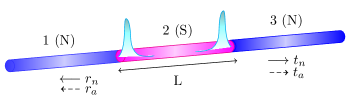
Figure 1: (Color online) Schematic picture of a NSN system. The middle part (2) with length $L$ is the $p$-wave superconductor, while the left and right parts (1 and 3) are normal metal leads. Four amplitudes are shown: $r_{n},~{}r_{a}$ are normal and Andreev reflections in the left lead, and $t_{n},~{}t_{a}$ are normal and Andreev transmissions in the right lead. Majorana modes at the two ends of the SC region are also shown.

Let us denote the wave function in each region as $\psi=(c,~{}d)^{T}$, where $c(x,t),~{}d(x,t)$ are the electron (particle) and hole components respectively (there is no spin label to be considered here). The Hamiltonian in each region can be written as

$$H = \int dx~{}[c^{\dagger}(-\frac{\hbar^{2}\partial_{x}^{2}}{2m}-\mu)c~{}-~{}d^{\dagger}(-\frac{\hbar^{2}\partial_{x}^{2}}{2m}-\mu)d$$ (1)

$$~{}~{}~{}~{}~{}~{}~{}~{}~{}-\frac{i\Delta}{k_{F}}~{}(c^{\dagger}\partial_{x}d+d^{\dagger}\partial_{x}c)],$$

where $\mu$ is the chemical potential, $k_{F}=\sqrt{2m\mu}/\hbar$ is the Fermi wave number, and $\Delta$ is the $p$-wave superconducting pairing amplitude assumed to be real everywhere; we will set $\Delta=0$ in the NM leads. (We will generally set $\hbar=1$ in this paper, except in places where it is required for clarity. The Fermi velocity is $v_{F}=\hbar k_{F}/m$). The Heisenberg equations of motion $i\partial_{t}c=-[H,c]$ and $i\partial_{t}d=-[H,d]$ imply that

$$i\partial_{t}c = (-\frac{\partial_{x}^{2}}{2m}-\mu)~{}c~{}-~{}\frac{i\Delta}{k_{F}}~{}\partial_{x}d,$$

$$i\partial_{t}d = (\frac{\partial_{x}^{2}}{2m}+\mu)~{}d~{}-~{}\frac{i\Delta}{k_{F}}~{}\partial_{x}c.$$ (2)

For a wave function which varies in space as $e^{ikx}$, the energy is given by $\pm(k^{2}/(2m)-\mu)$ if $\Delta=0$, and by $\pm\sqrt{(k^{2}/(2m)-\mu)^{2}+\Delta^{2}(k/k_{F})^{2}}$ if $\Delta\neq 0$. The corresponding wave functions will be presented below. We see that the energy spectrum in the SC has a gap equal to $2\Delta$ at $k=\pm k_{F}$.

Let us define the particle density $\rho_{p}=c^{\dagger}c+d^{\dagger}d$ and charge density $\rho_{c}=c^{\dagger}c-d^{\dagger}d$. Using Eqs. (2) and the equations of continuity $\partial_{t}{\rho_{p}}+\partial_{x}J_{p}=0$ and $\partial_{t}{\rho_{c}}+\partial_{x}J_{c}=0$, we find the particle and charge currents to be blonder ; soori

$$J_{p} = \frac{i}{2m}~{}[-~{}c^{\dagger}\partial_{x}c~{}+~{}\partial_{x}c^{\dagger}c~{}+~{}d^{\dagger}\partial_{x}d~{}-~{}\partial_{x}d^{\dagger}d]$$

$$~{}+~{}\frac{\Delta}{k_{F}}~{}(c^{\dagger}d+d^{\dagger}c),$$

$$J_{c} = J_{1}~{}+~{}\int_{0}^{x}dx^{\prime}~{}J_{2}(x^{\prime}),$$

$$J_{1} = \frac{i}{2m}~{}[-~{}c^{\dagger}\partial_{x}c~{}+~{}\partial_{x}c^{\dagger}c~{}-~{}d^{\dagger}\partial_{x}d~{}+~{}\partial_{x}d^{\dagger}d]$$

$$~{}+~{}\frac{\Delta}{k_{F}}~{}(c^{\dagger}d+d^{\dagger}c)],$$

$$J_{2} = -~{}\frac{2\Delta}{k_{F}}~{}(\partial_{x}c^{\dagger}d+d^{\dagger}\partial_{x}c).$$ (3)

The last term, $J_{2}$, can be interpreted as the contribution of Cooper pairs to the charge current; note that it vanishes in the NM where $\Delta=0$.

The boundary conditions at the SC-NM junctions at $x=0$ and $L$ can be found by demanding that the currents $J_{p}$ and $J_{c}$ be conserved at those points. At the junction $x=0$, let us consider the wave functions $\psi_{1}=(c_{1},~{}d_{1})^{T}$ and $\psi_{2}=(c_{2},~{}d_{2})^{T}$ at the points $x=0-\epsilon$ and $x=0+\epsilon$, i.e., in the NM and SC regions respectively. The condition $J_{p1}(0-\epsilon)=J_{p2}(0+\epsilon)$ implies that

$$\frac{i}{2m}~{}[-~{}c_{1}^{\dagger}\partial_{x}c_{1}~{}+~{}\partial_{x}c_{1}^{\dagger}c_{1}~{}+~{}d_{1}^{\dagger}\partial_{x}d_{1}~{}-~{}\partial_{x}d_{1}^{\dagger}d_{1}~{}]$$

$$= \frac{i}{2m}~{}[-~{}c_{2}^{\dagger}\partial_{x}c_{2}~{}+~{}\partial_{x}c_{2}^{\dagger}c_{2}~{}+~{}d_{2}^{\dagger}\partial_{x}d_{2}~{}-~{}\partial_{x}d_{2}^{\dagger}d_{2}]$$ (4)

$$~{}+~{}\frac{\Delta}{k_{F}}~{}(c_{2}^{\dagger}d_{2}+d_{2}^{\dagger}c_{2}).$$

The simplest way of satisfying this condition is to set

$$c_{1} = c_{2},$$

$$d_{1} = d_{2},$$

$$\partial_{x}c_{1} = \partial_{x}c_{2}~{}+~{}\frac{i\Delta}{v_{F}}~{}d_{2},$$

$$\partial_{x}d_{1} = \partial_{x}d_{2}~{}-~{}\frac{i\Delta}{v_{F}}~{}c_{2},$$ (5)

where $v_{F}=\hbar k_{F}/m$. (The first two equations above mean that the wave function is continuous while the last two equations imply that the first derivative is discontinuous in a particular way). We now find Eqs. (5) also imply that that charge current is conserved, i.e., $J_{c1}(0-\epsilon)=J_{c2}(0+\epsilon)$. Next, let us consider what happens if a $\delta$-function potential of strength $\lambda$ is also present at the junction at $x=0$; the dimension of $\lambda$ is energy times length. (This potential is physically motivated by the fact that in many experiments, the NM leads are weakly coupled, by a tunnel barrier, to the SC. This can be modeled by placing a $\delta$-function potential with a large strength at the junction). Now there will be an additional discontinuity in the first derivative at $x=0$; this is found by integrating over the $\delta$-function which gives

$$\partial_{x}\psi_{2}(0+\epsilon)~{}-~{}\partial_{x}\psi_{1}(0-\epsilon)~{}=~{}2m\lambda~{}\psi_{1}(0).$$ (6)

Hence Eqs. (5) must be modified to

$$c_{1} = c_{2},$$

$$d_{1} = d_{2},$$

$$\partial_{x}c_{1}~{}+~{}2m\lambda~{}c_{1} = \partial_{x}c_{2}~{}+~{}\frac{i\Delta}{v_{F}}~{}d_{2},$$

$$\partial_{x}d_{1}~{}+~{}2m\lambda~{}d_{1} = \partial_{x}d_{2}~{}-~{}\frac{i\Delta}{v_{F}}~{}c_{2}.$$ (7)

For the SC-NM junction at $x=L$, we consider the wave functions $\psi_{2}=(c_{2},~{}d_{2})^{T}$ at $x=L-\epsilon$ in the SC region and $\psi_{3}=(c_{3},~{}d_{3})^{T}$ at $x=L+\epsilon$ in the NM region. Assuming that there is also a $\delta$-function potential with strength $\lambda$ at this junction, we find that the boundary conditions which conserve the probability and charge current at this point are given by

$$c_{2} = c_{3},$$

$$d_{2} = d_{3},$$

$$\partial_{x}c_{2}~{}+~{}\frac{i\Delta}{v_{F}}~{}d_{2}~{}+~{}2m\lambda~{}c_{2} = \partial_{x}c_{3},$$

$$\partial_{x}d_{2}~{}-~{}\frac{i\Delta}{v_{F}}~{}c_{2}~{}+~{}2m\lambda~{}d_{2} = \partial_{x}d_{3}.$$ (8)

We now use the boundary conditions discussed above to find the various reflection and transmission amplitudes when an electron is incident from, say, the NM lead on the left with unit amplitude. The presence of the SC in the middle implies that one of four things can happen blonder .

(i) an electron can be reflected back to the left lead with amplitude $r_{n}$.

(ii) a hole can be reflected back to the left lead with amplitude $r_{a}$. In this case, charge conservation implies that a Cooper pair must be produced inside the SC.

(iii) an electron can be transmitted to the right lead with amplitude $t_{n}$.

(iv) a hole can be transmitted to the right lead with amplitude $t_{a}$. (This is usually called crossed Andreev reflection law2 ). Then charge conservation again implies that a Cooper pair must be produced inside the SC.

If the energy $E$ of the electron (incident from the left lead) lies in the superconducting gap, i.e., $-\Delta\leq E\leq\Delta$ ($E$ can be interpreted as the bias between the left lead and the SC), Eqs. (2) imply that the wave functions in the three regions must be of the form

$$\psi_{1} = e^{ikx}\left(\begin{array}[]{c}1\\ 0\end{array}\right)+r_{n}e^{-ikx}\left(\begin{array}[]{c}1\\ 0\end{array}\right)+r_{a}e^{ikx}\left(\begin{array}[]{c}0\\ 1\end{array}\right),$$ (15)

$$\psi_{2} = t_{1}e^{ik_{1}x}\left(\begin{array}[]{c}1\\ e^{i\phi}\end{array}\right)+t_{2}e^{ik_{2}x}\left(\begin{array}[]{c}1\\ -e^{-i\phi}\end{array}\right)$$ (25)

$$+~{}t_{3}e^{ik_{3}x}\left(\begin{array}[]{c}1\\ e^{-i\phi}\end{array}\right)+t_{4}e^{ik_{4}x}\left(\begin{array}[]{c}1\\ -e^{i\phi}\end{array}\right),$$

$$\psi_{3} = t_{n}e^{ikx}\left(\begin{array}[]{c}1\\ 0\end{array}\right)+t_{a}e^{-ikx}\left(\begin{array}[]{c}0\\ 1\end{array}\right),$$ (30)

where $e^{i\phi}=(E-i\sqrt{\Delta^{2}-E^{2}})/\Delta$. Here $\psi_{1}$ and $\psi_{3}$ are the wave functions in the NM leads on the left (1) and right (3) respectively, while $\psi_{2}$ is the wave function in the SC region in the middle (see Fig. 1). The top and bottom entries in the wave functions denote the particle and hole components. The wave functions in the NM leads are proportional to $e^{\pm ikx}$, where $k$ is close to the Fermi wave number $k_{F}$. In the SC, we have four modes; two of these decay exponentially and the other two grow as we move from left to right. We denote the wave numbers of these by $k_{1},~{}k_{2},~{}k_{3}$ and $k_{4}$. Defining the length scale

$$\xi~{}=~{}\frac{\hbar v_{F}}{\Delta\sqrt{1-(E/\Delta)^{2}}},$$ (31)

we find that the decaying modes have $k_{1}=k_{F}+i/\xi$ and $k_{2}=-k_{F}+i/\xi$, while the growing modes have $k_{3}=k_{F}-i/\xi$ and $k_{4}=-k_{F}-i/\xi$.

Upon including the $\delta$-function potentials with strength $\lambda$ at the junctions at $x=0$ and $x=L$, we get a total of eight boundary conditions from Eqs. (7) and (8) which connect $\psi_{1}=(c_{1},~{}d_{1})^{T}$, $\psi_{2}(c_{2},~{}d_{2})^{T}$ and $\psi_{3}=(c_{3},~{}d_{3})^{T}$. We thus have eight equations for the eight unknowns $r_{a},~{}r_{n},~{}t_{n},~{}t_{a},~{}t_{1},~{}t_{2},~{}t_{3}$ and $t_{4}$. After solving these equations we can calculate the reflection and transmission probabilities. The conservation law for probability current implies that

$$|r_{a}|^{2}~{}+~{}|r_{n}|^{2}~{}+~{}|t_{a}|^{2}~{}+~{}|t_{n}|^{2}~{}=~{}1.$$ (32)

The net probability of an electron to be transmitted from the left NM lead to the right NM lead gives the differential conductance

$$G_{N}~{}=~{}|t_{n}|^{2}~{}-~{}|t_{a}|^{2}.$$ (33)

The net probability of the electron to be reflected back to the left NM lead is

$$G_{B}~{}=~{}|r_{n}|^{2}~{}-~{}|r_{a}|^{2}.$$ (34)

The remainder, denoted by the differential conductance $G_{C}$, is the probability of electrons to be transmitted into the SC in the form of Cooper pairs. The conservation of charge current implies that

$$G_{C} = 1~{}-~{}G_{N}~{}-~{}G_{B}$$ (35)

$$= 2~{}(|r_{a}|^{2}~{}+~{}|t_{a}|^{2}),$$

where we have used Eqs. (32)-(34) to derive the last line in Eq. (35). The corresponding differential conductances into the right lead and the SC are given by $e^{2}/(2\pi\hbar)$ times $G_{N}$ and $G_{C}$, where $e$ is the charge of an electron. However, we will ignore the factors of $e^{2}/(2\pi\hbar)$ in this paper and simply refer to $G_{N}$ and $G_{C}$ as the conductances.

We note that a differential conductance denotes $G=dI/dV$. To measure $G_{N}$ and $G_{C}$ in our system, we have to assume that there is a voltage bias $V$ between the left NM lead on the one hand and the SC and the right NM lead on the other (the latter two are taken to be at the same potential). Namely, we choose the mid-gap energy in the SC as zero, and the Fermi energies in the left and right NM leads as $E=eV$ and zero respectively. The differential conductances $G_{N}=dI_{N}/dV$ and $G_{C}=dI_{C}/dV$ are then the derivatives with respect to $V$ of the currents measured in the right NM lead and in the SC.

III Numerical results for uniform $\Delta$

In this section we present our numerical results for $G_{N}$ and $G_{C}$ as functions of the length $L$ of the SC and the ratio $E/\Delta$ lying in the range $[-1,1]$. There is a length scale associated with the SC gap called $\eta=\hbar v_{F}/\Delta$. (This is different from the length $\xi$ introduced in Eq. (31) which depends on the energy $E$). We study three cases, namely, $L\ll\eta$, $L\sim\eta$ and $L\gg\eta$.

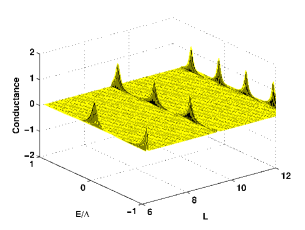
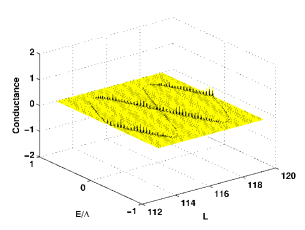
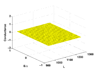
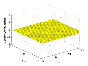
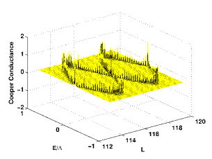
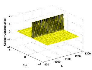
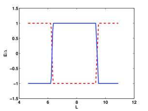
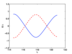
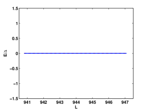
Figure 2: (Color online) Plots of conductances and energy splitting when $\Delta$ has the same sign everywhere in the SC: the parameters chosen are $k_{F}=1,~{}m=1,~{}\Delta=0.01,\lambda=10$, and an offset in $k_{F}L$ equal to $0.1$. Each row shows three plots corresponding, from left to right, to $L=2\pi-0.1~{}\text{to}~{}4\pi-0.1$, $L=37\pi-0.1~{}\text{to}~{}39\pi-0.1$, and $L=300\pi-0.1~{}\text{to}~{}400\pi-0.1$. Figures (a-c) show the conductance $G_{N}$ from the left lead to the right lead while figures (d-f) show the conductance $G_{C}$ from the left lead to the SC, as functions of $L$ and $E/\Delta$. In figures (a) and (d), with $L=2\pi-0.1~{}\text{to}~{}4\pi-0.1$, we see that $G_{C}$ is almost zero everywhere, while $G_{N}$ is a maximum at the values of $L$ where the quantization condition $k_{F}L=n\pi-\text{offset}$ is satisfied. (We do not see peaks in $G_{N}$ at all points on those lines because of the finite resolution of the set of values of $L$ and $E/\Delta$ that we have taken in our numerical calculations. As we increase the number of points, we do find that the peaks occupy an increasingly large fraction of those lines). In figures (b) and (e), with $L=37\pi-0.1~{}\text{to}~{}39\pi-0.1$, we see a sinusoidal variation in the locations of the peaks of both $G_{N}$ and $G_{C}$ as a function of $L$. In figures (c) and (f), with $L=300\pi-0.1~{}\text{to}~{}400\pi-0.1$, $G_{N}$ is almost zero everywhere, while $G_{C}$ has peaks only at $E/\Delta=0$ (zero bias peak) where its value is 2. Figures (g-i) show the analytically calculated energies $E/\Delta$ of the Majorana modes as a function of the length $L$ of a SC box. The conductance peaks in figures (a-f) occur exactly at the Majorana mode energies in the figures (g-i).

We show the numerically obtained conductances $G_{N}$ and $G_{C}$ in the first and second rows of Fig. 2. We have chosen the parameters $k_{F}=1,~{}m=1,~{}\Delta=0.01,~{}\lambda=10$, and an offset in $k_{F}L$ equal to $0.1$ (the reason for the offset is explained in Sec. IV.1). The length scale $\eta=\hbar^{2}k_{F}/(m\Delta)=100$. In the first column of Fig. 2, we have taken $L=2\pi-0.1~{}\text{to}~{}4\pi-0.1$, namely, $L\ll\eta$. We then find that $G_{N}$ is peaked at the values of $L$ where the quantization condition, $k_{F}L=n\pi-\text{offset}$, is satisfied, and $G_{C}$ is almost zero everywhere. For a fixed value of $k_{F}$, we find that the offset depends only on the strength of the $\delta$-function potential $\lambda$ as shown in Eq. (39) below. In the second column, we have taken $L=37\pi-0.1~{}\text{to}~{}39\pi-0.1$, i.e., $L\sim\eta$. Here we find that the locations of the peaks of both $G_{N}$ and $G_{C}$ vary sinusoidally with $L$. In the third column, we have taken $L=300\pi-0.1~{}\text{to}~{}400\pi-0.1$, i.e., $L\gg\eta$. Here $G_{C}$ has peaks only at zero energy (called the zero bias peak) where its value is 2, while $G_{N}$ is almost zero everywhere. The general pattern of variation of the conductances is that $G_{N}$ decreases while $G_{C}$ increases with increasing $L$. For very large $L$, we observe only a zero bias peak in $G_{C}$, and only the junction at $x=0$ is important; the electron never reaches the junction at $x=L$.

IV Analytical results for uniform $\Delta$

IV.1 Superconducting box

In this section, we study how the energies of the Majorana modes depend on the length $L$ of the SC region if the NM leads are absent. We consider a SC box with hard walls ($\lambda=\infty$) at $x=0$ and $L$. We therefore set the wave functions $\psi_{1}$ and $\psi_{3}$ equal to zero in Eq. (30) and consider only the wave function $\psi_{2}$. This satisfies a total of four boundary conditions, two at each wall.

At $x=0$, we obtain

$$t_{1}+t_{2}+t_{3}+t_{4} = 0,$$

$$t_{1}e^{i\phi}-t_{2}e^{-i\phi}+t_{3}e^{-i\phi}-t_{4}e^{i\phi} = 0,$$ (36)

while at $x=L$,

$$t_{1}e^{ik_{1}L}+t_{2}e^{ik_{2}L}+t_{3}e^{ik_{3}L}+t_{4}e^{ik_{4}L} = 0,$$

$$t_{1}e^{i\phi}e^{ik_{1}L}-t_{2}e^{-i\phi}e^{ik_{2}L}+t_{3}e^{-i\phi}e^{ik_{3}L}-t_{4}e^{i\phi}e^{ik_{4}L} = 0.$$

The consistency of these four equations implies the condition

$$\frac{E}{\Delta}~{}=~{}\pm~{}\frac{\sin(k_{F}L)}{\sqrt{\sin^{2}(k_{F}L)~{}+~{}\sinh^{2}(L/\xi)}}.$$ (38)

This splitting of the energy away from zero is essentially due to the hybridization of the Majorana modes due to a finite tunneling amplitude between the two ends of the SC box. We note that oscillations in the energy splitting due to the factor of $\sin(k_{F}L)$ have been studied in certain regimes of the wire length in Refs. sarma, , pientka2, , klino2, and stanescu4, . However, the analytical expression in Eq. (38) is valid for all values of $L$.

Note that in the limit $L/\xi\to\infty$, the energy splitting goes to zero, i.e., $E\to 0$. In this limit, the Majorana modes at the two ends of the box are decoupled from each other. The mode at the left end of the system ($x=0$) has a wave function of the form $(1,~{}-i)^{T}\sin(k_{F}x)e^{-x/\xi}$, while the mode at the other end $(x=L)$ has a wave function of the form $(1,~{}i)^{T}\sin(k_{F}(L-x))e^{-(L-x)/\xi}$. We have assumed so far that $\Delta>0$. If $\Delta<0$, we find that the mode at the left end is proportional to $(1,~{}i)^{T}$ while the mode at the right end is proportional to $(1,~{}-i)^{T}$.

[Incidentally, the wave functions of the Majorana modes can be made completely real by a unitary transformation. In Eq. (1), let us change the phases of $c$ and $d$ by $e^{i\pi/4}$ and $e^{-i\pi/4}$ respectively; this effectively changes the phase of $\Delta$ by $i$. We then find that the Majorana wave functions become $(1,~{}\pm 1)^{T}$ instead of $(1,~{}\pm i)^{T}$. Since their energy is zero, there is no complex phase factor $e^{-iEt}$. So the wave functions are real at all points in space and time].

To visualize the expression in Eq. (38), we show the dependence of $E/\Delta$ on $L$ in the third row of Fig. 2. For small values of $L/\eta\ll 1$, the energies are split by the maximum amount ($E/\Delta=\pm 1$), unless $k_{F}L$ is exactly equal to $n\pi$ where $E/\Delta=0$. As $L$ increases the splitting decreases as we see in Eq. (38) and in the second plot in the third row of Fig. 2. For $L/\eta\gg 1$, the energy splitting goes to zero as the tunneling between the two ends approaches zero exponentially with the length. We see that the analytical result in Eq. (38) matches with our numerical results.

We end this section by summarizing our understanding of the conductance peaks shown in Fig. 2. In the first column of that figure, the length $L$ of the superconducting part of the wire is small. Hence we can ignore the imaginary part, $\pm iL/\xi$, in the phase factors appearing in $\psi_{2}$ in Eq. (30). Thus the wave functions in the SC are approximately given by simple plane waves $e^{\pm ik_{F}x}$. Such a system has quantized energy levels when $k_{F}L=n\pi$; we then get transmission resonances, i.e., $|t_{n}|^{2}=1$ and $G_{N}=1$. $G_{C}$ is almost zero since the superconducting part is small. In the third column of Fig. 2, $L$ is much larger than the Majorana decay length $\xi$. The system therefore has zero energy Majorana modes near each end of the superconductor; the two modes are decoupled from each other since the Majorana wave functions decay exponentially as we go away from the ends, and $L$ is much larger than $\xi$. In this situation we find peaks in $G_{C}$ at zero bias since an electron coming in from the left lead can enter the superconductor by coupling to the Majorana mode; it then turns into a Cooper pair and a hole goes back into the left lead to conserve charge. We thus get perfect Andreev reflection, so that $|r_{a}|^{2}=1$ and $G_{C}=2$. $G_{N}$ is almost zero since the right lead is far away and the exponential decay of the wave function means the electron cannot reach there. In the second column of Fig. 2, $L$ has intermediate values of the same order as $\xi$; the Majorana modes at the two ends can now hybridize with each other. We have shown above that the Majorana wave functions oscillate as $\sin(k_{F}x)$ and $\sin(k_{F}(L-x))$. The hybridization between the Majorana modes at the two ends is proportional to the overlap of their wave functions and therefore oscillates with the length as $\sin(k_{F}L)$. Hence the energy splitting and therefore the peaks in $G_{N}$ and $G_{C}$ also oscillate as $\sin(k_{F}L)$.

IV.2 Conductances

In this section, we will present the exact forms of $G_{N}$ and $G_{C}$ in some special cases. It is generally difficult to analytically solve the eight equations coming from Eqs. (7)-(8). But if $E=0$ which implies that $e^{i\phi}=-i$ and $\xi=\hbar v_{F}/\Delta$, and if $\Delta\ll\hbar^{2}k_{F}^{2}/m$, it turns out that one can analytically solve the eight equations in two limits.

(i) If $\lambda/(\hbar v_{F})\gg 1$ but $e^{L/\xi}$ has a finite value, the numerical calculations of $r_{n},~{}r_{a},~{}t_{n}$ and $t_{a}$ show that for most values of the length $L$, $|r_{n}|\simeq 1$ and the other three amplitudes almost vanish; hence $G_{N},~{}G_{C}$ are very small. However, we find numerically that there are special values of $L$ where $r_{n},~{}t_{a}$ are almost equal to zero. We can then use this numerical observation and the boundary conditions to analytically find the quantization condition on $L$. We find that

$$e^{i2k_{F}L} = -~{}\frac{v_{F}+i\lambda}{v_{F}-i\lambda},$$

$${\rm implying~{}that}~{}~{}k_{F}L = n\pi-\theta,$$

$${\rm where}~{}~{}\theta \simeq \frac{\hbar v_{F}}{\lambda},$$

$${\rm and}~{}~{}|r_{a}| = \tanh~{}(\frac{L}{\xi}),$$

$$|t_{n}| = {\rm sech}~{}(\frac{L}{\xi}).$$ (39)

Hence $G_{N}={\rm sech}^{2}(L/\xi)$ and $G_{C}=2\tanh^{2}(L/\xi)$. We see that if $L/\xi\to 0$, $G_{N}\to 1$ and $G_{C}\to 0$, while if $L/\xi\to\infty$, $G_{N}\to 0$ and $G_{C}\to 2$. (Results similar to Eqs. (39) have been derived in Ref. lobos2, ).

Eq. (39) shows that if $\lambda$ is large but not infinite, there is a small offset equal to $\theta$ from the quantization condition $k_{F}L=n\pi$ which is true for $\lambda=\infty$ (as we see in Eq. (38) for $E=0$); hence $\sin(k_{F}L)$ is non-zero but small. For $k_{F}=1,~{}m=1$ and $\lambda=10$, we see that $\theta=0.1$, which matches with the numerical results shown in Sec. III.

(ii) If $\lambda/(\hbar v_{F})$ and $e^{L/\xi}$ are both much larger than 1 and $\sin(k_{F}L)$ is not small (i.e., $k_{F}L$ is not close to an integer multiple of $\pi$), we analytically find that

$$|r_{n}| = \frac{\nu^{2}}{1~{}+~{}\nu^{2}},$$

$$|r_{a}| = \frac{1}{1~{}+~{}\nu^{2}},$$

$$|t_{n}| = |t_{a}|~{}=~{}\frac{|\nu|}{1~{}+~{}\nu^{2}},$$

$${\rm where}~{}~{}\nu = \left(\frac{2\lambda}{\hbar v_{F}}\right)^{2}~{}e^{-L/\xi}~{}\sin(k_{F}L).$$

$${\rm Hence}~{}~{}G_{N} = 0~{}~{}{\rm and}~{}~{}G_{C}~{}=~{}\frac{2}{1~{}+~{}\nu^{2}}.$$ (40)

We see that if $\nu\to\infty$, $G_{C}\to 0$, while if $\nu\to 0$, $G_{C}\to 2$. There is a cross-over from one limit to the other depending on whether $(\lambda/\hbar v_{F})^{2}$ (the square of the strength of the barrier between the SC and the NM) is much larger than or much smaller than $e^{L/\xi}$.

V Effects of $\Delta$ changing sign

V.1 Continuum model

In this section, we will consider a continuum model for a system in which the $p$-wave pairing amplitude $\Delta$ changes sign at some point in the SC as shown in Fig. 3. (A way of experimentally realizing such a system will be discussed in Sec. VII). We now get twelve boundary conditions: four at the NM-SC junction at $x=0$, four at the SC-NM junction at $x=L$, and four at the point in the SC where $\Delta$ changes sign.

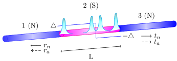
Figure 3: (Color online) Schematic picture of a NSN system where $\Delta$ changes sign at one point in the SC. The middle part with length $L$ is the $p$-wave superconductor, while the left and right parts are normal metal leads. $r_{n},~{}r_{a}$ are normal and Andreev reflection amplitudes in the left lead, and $t_{n},~{}t_{a}$ are normal and Andreev transmission amplitudes in the right lead. Also shown are four Majorana modes, two at the ends of the SC region and two near the point where $\Delta$ changes sign.

Using the boundary conditions we numerically calculate the conductances. These are shown in Fig. 4 for the parameter values $k_{F}=1,~{}m=1$, $\lambda=10$, and an offset in $k_{F}L=0.1$ where $L$ is the length of the SC. We take $\Delta=0.01$ from $x=0$ to $3L/4$, and $\Delta=-0.01$ from $x=3L/4$ to $L$. (We found numerically that if $\Delta$ changes sign exactly at the mid-point of the SC, the system has an extra symmetry which gives rise to a rather unusual pattern of conductances. Since experimentally the sign change will typically not occur at the mid-point, we chose it to be at $3L/4$ where there is no special symmetry). As in Sec. III where $\Delta$ was assumed to have the same sign everywhere in the SC, we consider three cases. For $L=2\pi-0.1~{}\text{to}~{}3\pi-0.1$, i.e., $L\ll\eta$, we get peaks in $G_{N}$ at those values of $L$ where the quantization condition $k_{F}L=(n\pi-\text{offset}$) is satisfied; $G_{C}$ is almost zero. For $L=36\pi-0.1~{}\text{to}~{}38\pi-0.1$, i.e., $L\sim\eta$, we find a sinusoidal variation of the locations of the peaks in both $G_{N}$ and $G_{C}$ as functions of $L$. For $L=300\pi-0.1~{}\text{to}~{}400\pi-0.1$, i.e., $L\gg\eta$, we find that $G_{N}$ is almost zero but $G_{C}$ has peaks only at zero energy where its value is 2. Thus the conductances show very similar behaviors as functions of $L$ and $E/\Delta$ for $\Delta$ having the same sign throughout the SC or changing sign at one point in the SC.

Although the conductances show similar behaviors for systems in which $\Delta$ has the same sign everywhere or changes sign at one point, we will show below that there is a difference in the Majorana mode structure in the two cases. Namely, if $\Delta$ changes sign at one point in the SC, two Majorana modes will generally appear near that point. But if $\Delta$ has the same sign everywhere, Majorana modes generally do not appear inside the SC unless a large impurity potential is present at one point (which has the effect of dividing the SC into two regions).

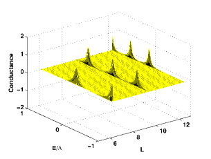
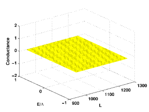
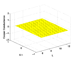
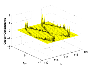
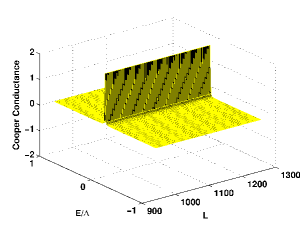
Figure 4: (Color online) Plots of conductances when $\Delta$ changes sign at one point in the SC: the parameters chosen are $k_{F}=1,~{}m=1,~{}\Delta=0.01,~{}\lambda=10$, and an offset in $k_{F}L$ equal to $0.1$. The first and second rows respectively show the conductance $G_{N}$ from the left lead to the right lead and the conductance $G_{C}$ from the left lead to the SC, as functions of $L$ and $E/\Delta$. The three different plots in the first two rows are for different ranges of $L$. The first column shows $L=2\pi-0.1~{}\text{to}~{}4\pi-0.1$, the second column shows $L=36\pi-0.1~{}\text{to}~{}38\pi-0.1$, and the third column shows $L=300\pi-0.1~{}\text{to}~{}400\pi-0.1$.

V.2 Kitaev chain

In this section we will obtain a clearer picture of the Majorana modes by studying the Kitaev chain. This is a lattice model of spinless $p$-wave SC with nearest neighbor hopping $\gamma$ (which we will assume to be positive), SC pairing $\Delta$, and chemical potential $\mu$. (Numerically, it is easier to study a lattice model than a continuum one). The Hamiltonian is

$$H= - \frac{i}{2}~{}\sum_{n=1}^{\mathcal{N}-1}~{}\Big{[}(\gamma-\Delta)~{}a_{n}b_{n+1}~{}+~{}(\gamma+\Delta)~{}a_{n+1}b_{n}\Bigl{]}$$ (41)

$$- \frac{i}{2}~{}\sum_{n=1}^{\mathcal{N}}~{}\mu~{}a_{n}b_{n},$$

where $a,b$ are Majorana operators which are Hermitian and satisfy the anticommutation relations $\{a_{m},a_{n}\}=\{b_{m},b_{n}\}=2\delta_{mn}$ and $\{a_{m},b_{n}\}=\delta_{mn}$. To connect this Majorana formalism to the usual particles, we define the particle creation and annihilation operators as $f_{n}=(1/2)(a_{n}-ib_{n})$ and $f_{n}^{\dagger}=(1/2)(a_{n}+ib_{n})$, which satisfy the standard anticommutation relations $\{f_{m},f_{n}^{\dagger}\}=\delta_{mn}$. The particle number operator at site $n$ is then given by $f_{n}^{\dagger}f_{n}=(ia_{n}b_{n}+1)/2$. Hence the last term in Eq. (41) is, apart from a constant, equal to $-\mu\sum_{n}f_{n}^{\dagger}f_{n}$, as a chemical potential term should be.

The Hamiltonian in Eq. (41) has an “effective time reversal symmetry”, namely, it is invariant under complex conjugation of all complex numbers along with $a_{n}\to a_{n}$ and $b_{n}\to-b_{n}$ manisha . (This symmetry would be violated if terms like $ia_{m}a_{n}$ or $ib_{m}b_{n}$ were present). This symmetry implies that if we look at eigenstates with zero energy, their wave functions involve only the $a_{n}$ or only the $b_{n}$, not both. Depending on the values of the parameters $\gamma,~{}\Delta$ and $\mu$, Eq. (41) is known to have two topological phases (for $|\mu|<\gamma$ and $\Delta\neq 0$) and one non-topological phase (for $|\mu|>\gamma$). The bulk modes are gapped in all the phases. In the topological phases, a long system has one zero energy Majorana mode at each end, whose wave functions involve only the $a_{n}$ operators near the left end and only the $b_{n}$ operators near the right end if $\Delta>0$, and vice versa if $\Delta<0$ manisha . (We can see this particularly clearly in the special case that $\mu=0$ and $\Delta=\pm\gamma$. If $\Delta=\gamma$ ($-\gamma$), the Majorana modes are given by $a_{1}$ ($b_{1}$) at the left end and $b_{\mathcal{N}}$ ($a_{\mathcal{N}}$) at the right end). Comparing these statements with the expressions given in the paragraph following Eq. (38) for the wave functions of Majorana modes at the ends of a long system, we conclude that a Majorana mode made from $a_{n}$ ($b_{n}$) has a wave function of the form $(1,-i)^{T}$ ($(1,i)^{T}$).

The energies and eigenstates of Eq. (41) have some interesting properties. We can write the Hamiltonian in the general form

$$H~{}=~{}i~{}\sum_{mn}~{}\alpha_{m}M_{mn}\alpha_{n},$$ (42)

where $M_{mn}$ is a real antisymmetric matrix, and $\alpha_{n}$ denote all the $2{\mathcal{N}}$ Majorana operators. The energies $E$ and corresponding eigenstates $u$ must satisfy $iMu=Eu$. We then see that for every non-zero energy $E$ and eigenstate $u$, there will be an energy $-E$ with eigenstate $u^{*}$. Next, the fact that the Hamiltonian only has terms like $ia_{m}b_{n}$ implies that we can choose the eigenstates in such a way that the $a_{n}$ components are real and the $b_{n}$ components are imaginary. Hence, when we go from $u$ to $u^{*}$, the $a_{n}$ components will remain the same while the $b_{n}$ components change sign. This implies that the quantity $ia_{n}b_{n}$, which is related to the particle number $f_{n}^{\dagger}f_{n}$ at site $n$, has opposite signs for the states $u$ and $u^{*}$ with energies $E$ and $-E$.

To numerically study the Majorana modes in this system, we first consider a 500-site system with $\gamma=1,~{}\Delta=0.03$, and $\mu=0.9$. To distinguish between localized and extended states, we use the inverse participation ratio (IPR) mt . (Given an eigenstate $\psi$ of the Hamiltonian, which is normalized so that $\sum_{n}|\psi_{n}|^{2}=1$, the IPR of the state is defined as $\sum_{n}|\psi_{n}|^{4}$). We find that for two of the eigenstates, the IPR is much larger than for all the other eigenstates; these correspond to localized states. The energy eigenvalues of these two eigenstates are zero to our numerical accuracy. Hence we get one Majorana mode at each end of the system as shown in Fig. 5. Note that the number of components of the wave function is twice the number of sites since each site $n$ has $a_{n}$ and $b_{n}$.

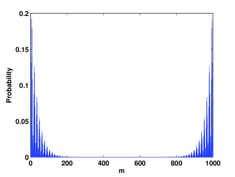
Figure 5: (Color online) Two Majorana modes, one at each end of a 500-site system with $\gamma=1,~{}\Delta=0.03$, and $\mu=0.9$.

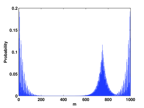
Figure 6: (Color online) Four Majorana modes, one at each end and two in the middle (on two sides of the components around 700 corresponding to the site labeled 350), for a 500-site system with $\gamma=1$, $\mu=0.9$, and $\Delta=0.03$ for sites 1 to 350 and $-0.03$ for sites 351 to 500.

Next we again consider a 500-site system with $\gamma=1$ and $\mu=0.9$, but now with $\Delta=0.03$ from site 1 to 350 and $\Delta=-0.03$ from site 351 to 500. The IPR is maximum for four eigenstates, indicating the presence of localized state. The energy eigenvalues of these four eigenstates are zero to numerical accuracy. The system now has four Majorana modes as shown in Fig. 6: two at the ends and two around the point where $\Delta$ changes sign. (Note that the wave function components $m=699,~{}700$ correspond to $a_{n}$ and $b_{n}$ at the site labeled $n=350$). We note that in Figs. 5 and 6, there is no impurity potential anywhere inside the system.

It is important to note that a SC in which $\Delta$ changes sign at one point, say $x=x_{0}$, will necessarily have two Majoranas near that point if the Hamiltonian only has terms of the form $ia_{m}b_{n}$. To see this, note that if the SC was cut at that point by putting an infinitely strong barrier there, the left part of the SC where $\Delta>0$ will have a Majorana involving $a_{n}$ at its left end (i.e., at $x=-\infty$) and $b_{n}$ at its right end ($x=x_{0}$), while the right part of the SC where $\Delta<0$ will have a Majorana involving $b_{n}$ at its left end (at $x=x_{0}$) and $a_{n}$ at its right end ($x=\infty$). We thus see that there will be two Majoranas near $x=x_{0}$ which are both of type $b$. If the barrier at $x=x_{0}$ is now decreased to a finite value (or even removed), the two Majoranas will survive since the Hamiltonian has no terms of type $ib_{m}b_{n}$ which can couple them and thereby gap them out. This is different from a SC where $\Delta$ has the same sign everywhere. Then an infinitely strong barrier at some point $x_{0}$ will cut the SC and produce two zero energy Majoranas there, but these will be of opposite types, $a$ and $b$. Lowering the barrier will now mix these Majoranas by tunneling and thus gap them out if the barrier is small enough. These observations are illustrated in Figs. 7 and 8.

Fig. 7 shows some of the eigenvalues for a 500-site system with different values of $\lambda$, which is the strength of an impurity placed at the site labeled 350. The energies are sorted in increasing order and are labeled by $m$ which runs from 1 to 1000. Thus $m=500,~{}501$ label the middle two energy levels; these remain at zero for all values of $\lambda$ and correspond to Majorana modes at the ends of the SC. The Majorana modes near the site labeled 350 correspond to $m=499,~{}502$; they are at zero energy if $\lambda$ is large but move away from zero and merge with the bulk states as $\lambda$ is decreased.

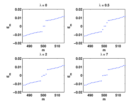
Figure 7: (Color online) Energy levels for different values of the strength $\lambda$ of an impurity inside a SC, when $\Delta$ has the same value everywhere. The system has 500 sites, $\gamma=1,~{}\mu=0.9$, and $\Delta=0.03$ at all sites. The impurity with strength $\lambda$ is at the site labeled 350. For small $\lambda$, there are only two Majorana modes, with energy close to zero, which lie at the ends of the SC. For large $\lambda$, the SC gets cut into two parts, and two additional Majorana modes appear near the impurity.

The situation is different if $\Delta$ changes sign at one point in the SC and there is also an impurity at the point. The number of Majorana modes close to zero energy is now always four regardless of the value of $\lambda$; two of the modes lie at the ends of the system and the other two lie near the point where $\Delta$ changes sign (these modes were shown in Fig. 6 for the case $\lambda=0$). Fig. 8 shows the energies of these four modes for a 500-site system with $\Delta$ changing sign and an impurity of strength $\lambda$ at the site labeled 350. We see that the four energies lie close to zero for all $\lambda$, unlike Fig. 7 where that happens only if $\lambda$ is large.

Figure 8: (Color online) Energy levels for different values of the strength $\lambda$ of an impurity inside a SC, when $\Delta$ changes sign at that point. The system has 500 sites, $\gamma=1,~{}\mu=0.9$, and $\Delta=0.03$ for sites 1 to 350 and $-0.03$ for sites 351 to 500. The impurity with strength $\lambda$ is at the site labeled 350. For all values of $\lambda$, there are four Majorana modes with energy close to zero, two of which lie at the ends of the SC and two are near the site where $\Delta$ changes sign.

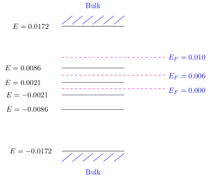
Figure 9: (Color online) Energy spectrum for a 60-site system with $\gamma=1$, $\mu=0.9$, and $\Delta=0.03$ from sites 1 to 45 and $-0.03$ from sites 45 to 60. The three values of $E_{F}$ shown correspond to the three plots in Fig. 10.

We will now look at the effect of the Majorana modes on the local particle density. Let $a_{E,n}$ and $b_{E,n}$ denote the $a$ and $b$ components of an eigenstate with energy $E$. For a Fermi energy $E_{F}$, all energy levels up to $E_{F}$ will be filled. We then define the total particle density at each site $n$ as

$$\rho_{n}~{}=~{}\frac{1}{2}\sum_{E<E_{F}}(ia_{E,n}b_{E,n}~{}+~{}1),$$ (43)

where $E_{F}$ is the Fermi energy of the system and $n$ goes from 1 to $\mathcal{N}$. We consider a system of size $\mathcal{N}=60$, $\gamma=1,~{}\mu=0.9$, with $\Delta$ equal to $0.03$ from sites 1 to 45 and $-0.03$ from sites 45 to 60. This system size is not very large, so the four Majorana modes will hybridize with each other and their energies will split from zero. We find numerically that the energies of the four modes lie at $\pm 0.0086$ and $\pm 0.0021$ as shown in Fig. 9. The bulk gap is found to be $0.0344$, so these four energies lie well within the bulk gap. We now study the particle density given in Eq. (43) for three values of Fermi energy $E_{F}=0.010,0.006,0.000$ to see the effect of the Majorana modes on the particle density. For $E_{F}=0.010$, the PD does not get any contribution from Majorana modes as the contributions to $ia_{n}b_{n}$ from pairs of states with energies $\pm E$ cancel out. For $E_{F}=0.006$, the PD gets contribution only from one unpaired Majorana mode (with $E=-0.0086$). For $E_{F}=0.000$, PD gets contribution from both the unpaired Majorana modes ($E=-0.0086$ and $-0.0021$). The PD for these three values of $E_{F}$ is shown in Fig. 10. A comparison of the three plots will show the contribution of the Majorana modes to the PD; for instance, the difference of the PD in plots (a) and (b) comes from the Majorana mode at $E=-0.0086$ while the difference of the PD of the plots (b) and (c) comes from the Majorana mode at $E=-0.0021$.

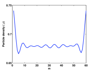
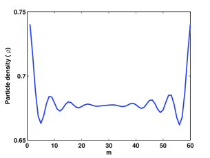
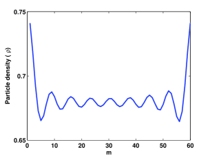
Figure 10: (Color online) Plots of the particle density when $\Delta$ changes sign at one point in the SC. We take the the SC region to have 60 sites, with $\gamma=1$, $\mu=0.9$, $\Delta=0.03$ from sites 1 to 45, and $\Delta=-0.03$ from sites 45 to 60. As the system length is finite, the four Majorana modes (two near the ends and two near the $45$-th site) split from zero energy. The energies of the four modes are $\pm 0.0086$ and $\pm 0.0021$. Figure (a) is for $E_{F}=0.010$ which lies above all the Majorana energies; hence the PD does not get a contribution from any of the Majorana modes since they are all occupied but their contributions cancel out in pairs. Figure (b) is for $E_{F}=0.006$; here the PD gets a contribution only from the Majorana mode at $E=-0.0086$ since the mode at $E=0.0086$ is unoccupied and therefore does not contribute. Figure (c) is for $E_{F}=0.000$; now the PD gets contributions from the Majorana modes at both $E=-0.0086$ and $-0.0021$ since the modes at $E=0.0086$ and $0.0021$ are unoccupied and do not contribute.

VI Interactions and renormalization group analysis

We will now study the effect of interactions between the electrons on the Majorana modes. More precisely, we will use the RG method to study how the various parameters of the model vary with the length scale, and we will then use that to see what happens to the Majorana modes. To begin, we will study only the SC region and not the NM leads. At the end of this section, we will consider the RG equation for a tunnel barrier lying at the junction of a SC and a NM.

Interactions have a particularly strong effect on many-electron systems in one dimension. Short range interactions change the system from a Fermi liquid to a Tomonaga-Luttinger liquid (TLL). The most effective way to study a TLL is to use bosonization gogolin ; delft ; rao ; giamarchi . Let us briefly explain the bosonization formalism. We first expand the second quantized electron fields around the Fermi wave numbers $\pm k_{F}$ as

$$\Psi~{}=~{}e^{ik_{F}x}~{}\Psi_{R}~{}+~{}e^{-ik_{F}x}~{}\Psi_{L},$$ (44)

where $\Psi_{R}$ and $\Psi_{L}$ denote right and left moving linearly dispersing fields. In bosonization these are related to two conjugate bosonic fields $\phi$ and $\theta$ as

$$\Psi_{R/L}~{}\sim~{}\frac{1}{\sqrt{2\pi a_{0}}}~{}\exp[i\sqrt{\pi}~{}(\mp\phi+\theta)],$$ (45)

where $a_{0}$ is a microscopic length scale such as the lattice spacing or the distance between nearest neighbor particles. (For simplicity we are ignoring Klein factors in Eq. (45)). The fields $\phi$ and $\theta$ describe particle-hole excitations, and their space-time derivatives give the charge current $J_{c}$ and the deviation of the charge density from a uniform background density, $\delta\rho=\rho_{c}-\rho_{0}$. Short range density-density interactions of the form $\int\int dxdy\rho(x)V_{int}(x-y)\rho(y)$ are therefore quadratic in terms of $\phi$ and $\theta$; this is the key advantage of the bosonization formalism. The Dirac Hamiltonian $H=iv_{F}\int dx[-\Psi_{R}^{\dagger}\partial_{x}\Psi_{R}+\Psi_{L}^{\dagger}\partial_{x}\Psi_{L}]$ (here $v_{F}$ is the Fermi velocity of the non-interacting system of electrons) along with density-density interactions takes the bosonic form $H=(v/2)\int dx[K(\partial_{x}\theta)^{2}+(\partial_{x}\phi)^{2}/K]$, where $v$ is the velocity of the particle-hole excitations in the interacting theory, and $K$ is a dimensionless parameter called the Luttinger parameter; these are related to $v_{F}$ and the strength of the interactions. [For repulsive (attractive) interactions between the electrons, $K<1$ ($K>1$)]. The superconducting term $\Psi_{R}^{\dagger}\Psi_{L}^{\dagger}$ plus its Hermitian conjugate is proportional to $\sin(2\sqrt{\pi}\theta)$. Finally, if we have a lattice model which is at half filling, there will be umklapp scattering terms like $\Psi_{R}^{\dagger}\Psi_{R}^{\dagger}\Psi_{L}\Psi_{L}e^{-i4k_{F}x}$ plus its Hermitian conjugate which add up to $\cos(4\sqrt{\pi}\phi-4k_{F}x)$. Putting all this together, we get a bosonized Hamiltonian of the form giamarchi ; ganga

$$H = \int\frac{dx}{2}[~{}vK(\partial_{x}\theta)^{2}~{}+~{}\frac{v}{K}(\partial_{x}\phi)^{2}~{}+~{}\frac{4\delta}{\pi a_{0}^{2}}~{}\sin(2\sqrt{\pi}\theta)$$ (46)

$$~{}~{}~{}~{}~{}~{}~{}~{}~{}-~{}\frac{U}{\pi^{2}a_{0}^{2}}~{}\cos(4\sqrt{\pi}\phi-4k_{F}x)],$$

where $\delta$ is related to the SC pairing $\Delta$ as $\delta=\Delta a_{0}$ at the microscopic length scale (we will see below that all these quantities will change with the length scale). We will ignore the umklapp scattering term below by setting $U=0$.

Let us consider the case where there is an isolated impurity in the system; for simplicity, we will assume this to be point-like so that the impurity potential is $V(x)=\lambda\delta(x)$, $\lambda$ being the strength of the impurity. The Hamiltonian which describes the effect of this is given by

$$H_{imp}~{}=~{}\int dx~{}V(x)\rho(x)~{}=~{}\lambda\rho(0),$$

where the density $\rho(x)=-(1/\pi)\partial_{x}\phi(x)$. The interaction renormalizes the system parameters. Hence the RG equations for the length scale dependence of the parameters $K$, $\delta$ and $\lambda$ are given by

$$\frac{dK}{dl} = \frac{\delta^{2}}{2},$$

$$\frac{d\delta}{dl} = (2-\frac{1}{K})~{}\delta,$$

$$\frac{d\lambda}{dl} = (1-K)~{}\lambda.$$ (48)

It is convenient to define a renormalized length scale $a=a_{0}e^{l}$. In the figures below, we will plot the pairing $\Delta$ which is related to $\delta$ as $\Delta=\delta/a$; this satisfies the equation $d\Delta/dl=(1-1/K)\Delta$. It is $\Delta$, rather than $\delta$, which is physically observable; for instance $\Delta$ is the superconducting gap for a system with length scale $a$. Note that for a non-interacting system, i.e., $K=1$, both $\delta$ and $a$ flow, but $\Delta$ does not flow. We note that the first two equations in Eqs. (48) were studied in Ref. ganga, . We have generalized their analysis by introducing an impurity with strength $\lambda$ which flows according to the last equation in Eqs. (48). It is important for us to consider this equation since we are mainly interested in the conductances of the system and these are strongly affected by the presence of impurities or barriers (see Eq. (50)). As we will see below, an impurity inside a SC region can have interesting consequences for Majorana modes and the conductances.

We have used the RG equations and some initial values of the parameters $K$, $\Delta/\Delta_{0}$ and $\lambda$ to find how these parameters vary with the length scale. These are shown in Figs. 11 and 12 for initial values $K_{0}=0.8$ (repulsive interactions) and $K_{0}=1.2$ (attractive interactions) respectively, along with $\Delta_{0}=0.01$ and $\lambda_{0}=2$. For $K<1$, $\lambda$ increases and $\Delta$ decreases with increasing length scale,and these trends are reversed when $K>1$. In Fig. 11, where $K_{0}=0.8$, we see that $\lambda$ keeps increasing up to $l=6$ (beyond this $K$ becomes larger than 1). These results have the following implications for Majorana modes at the ends of the SC.

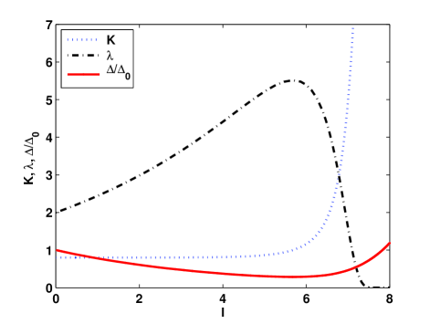
Figure 11: (Color online) Plots of $K$, $\Delta/\Delta_{0}$ and $\lambda$ versus $l$. The initial values of the parameters are $\Delta_{0}=0.01$, $K_{0}=0.8$ and $\lambda_{0}=2$.

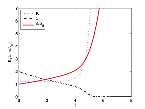
Figure 12: (Color online) Plots of $K$, $\Delta/\Delta_{0}$ and $\lambda$ versus $l$. The initial values of the parameters are $\Delta_{0}=0.01$, $K_{0}=1.2$ and $\lambda_{0}=2$.

If there is no impurity inside the SC (i.e., $\lambda=0$), then we will be in the situation studied in Ref. ganga, . If the SC region has a length $L$, the Majorana modes survive if the value reached by $\Delta$ at that length scale satisfies $L\Delta/v\gg 1$. If $L\Delta/v\lesssim 1$, the Majorana modes will hybridize strongly and move away from zero energy; if their energies approach the ends of the SC gap at $\pm\Delta$, they will become unobservable.

If $\lambda\neq 0$, it will grow with the length scale if $K<1$. For a large impurity strength $\lambda$ at one point, the SC essentially gets cut into two parts and one can get two Majorana modes on the two sides of that point stanescu4 . As shown in Fig. 7 for a 500-site system, the energies of these Majorana modes approach zero as $\lambda$ becomes large. (As discussed below, the RG equations cannot be trusted up to very large values of $\lambda$. The largest value $\lambda=7$ shown in Figs. 7 and 8 is therefore only for the purposes of illustration and may not be physically realistic). The situation is different if $\Delta$ changes sign at one point in the SC and there is also an impurity at the point. The RG equations will be the same as discussed above for the case of uniform $\Delta$. However the number of Majorana modes is now always four regardless of the value of $\lambda$. Two of the modes lie at the ends of the system and the other two lie near the point where $\Delta$ changes sign; the energies of these four modes are shown in Fig. 8. We see that the four energies lie close to zero for all $\lambda$.

We have studied above what happens if there is an impurity of strength $\lambda$ which lies inside the SC. It is also interesting to study the RG flow of an impurity which lies at the ends of the SC region, namely, the barriers which lie at the junctions between the SC and a NM lead. It is known that an impurity of strength $\lambda$ lying at the junction between two different TLLs with Luttinger parameters $K_{1}$ and $K_{2}$ satisfies the RG equation

$$\frac{d\lambda}{dl}~{}=~{}(1~{}-~{}\frac{2K_{1}K_{2}}{K_{1}~{}+~{}K_{2}})~{}\lambda.$$ (49)

Since a NM is equivalent to a TLL with $K=1$, the RG equation for the strength of an impurity at the junction between a NM and a SC which has a value of $K$ is given by

$$\frac{d\lambda}{dl}~{}=~{}\frac{1~{}-~{}K}{1~{}+~{}K}~{}\lambda.$$ (50)

If $K<1$, we see that a barrier strength $\lambda$ will increase with the length scale, though not as fast as the $\lambda$ of an impurity lying inside the SC as shown by the last equation in Eq. (48).

We can apply Eq. (50) to understand the conductance across a NSN system if we take $\lambda$ to be the strength of the tunnel barriers between the SC and the NM leads. If both $\lambda$ and $e^{L/\xi}$ are large and $k_{F}L$ is not an integer multiple of $\pi$, Eqs. (40) give expressions for the conductances across a NSN system at zero bias. For $E=0$, $L/\xi=L\Delta/v$; hence the parameter $\nu$ in Eqs. (40) depends on $\lambda$ and $\Delta$ both of which flow under RG. If $K<1$, $\lambda$ increases and $\Delta$ decreases with increasing length scales; both these imply that $\nu$ will increase and hence $G_{C}$ will decrease as the length $L$ of the SC is increased.

We would like to emphasize here that we have only discussed RG equations up to the lowest possible order in $\delta$ and $\lambda$. Hence the RG flows cannot be trusted when these parameters reach values of the order of the energy cut-off, namely, the Fermi energy. Hence we cannot definitely conclude that the RG flow will cut the wire into two parts. However, we can conclude that an impurity inside the superconducting part of the system will grow and may thereby give rise to additional sub-gap modes near that point in the case where the $p$-wave pairing $\Delta$ has the same sign everywhere. (If $\Delta$ changes sign at one point, two additional Majorana modes will appear there regardless of whether or not there is a barrier there, as we have argued on symmetry grounds).

VII Experimental realizations

We will now discuss how the different systems that we have discussed above can be experimentally realized. In particular, we will see how it may be possible to have a SC in which the pairing $\Delta$ changes sign at one point.

We consider the model studied in Ref. ganga, . We take a wire with a Rashba spin-orbit coupling of the form $\pm\alpha_{R}p_{r}\sigma^{x}$, where $p_{r}$ is the momentum along the wire and $\sigma^{x}$ is a Pauli spin matrix. This form can be justified as follows. Let us take the coordinate in the wire to increase along an arbitrary direction $\hat{r}$ lying in the $x-y$ plane (instead of the $\hat{x}$ direction as assumed in earlier sections). If the Rashba term is $\alpha_{R}{\hat{n}}\cdot{\vec{\sigma}}\times{\vec{p}}$, and $\hat{n}$ points in the $\hat{z}$ direction, then the Rashba term will be $\alpha_{R}p_{r}\sigma^{x}$ if ${\hat{r}}={\hat{y}}$ and $-\alpha_{R}p_{r}\sigma^{x}$ if ${\hat{r}}=-{\hat{y}}$.

Next, the wire is placed in a magnetic field in the $\hat{z}$ direction which is perpendicular to the Rashba term (with a Zeeman coupling $\Delta_{Z}$) and in proximity to a bulk $s$-wave SC with pairing $\Delta_{S}$. The complete Hamiltonian, given in Ref. ganga, , is

$$H = \int dr~{}\Psi^{\dagger}_{\alpha}\left[(\frac{p_{r}^{2}}{2m}-\mu)\delta_{\alpha\beta}\pm\alpha_{R}p_{r}\sigma^{x}_{\alpha\beta}-\Delta_{Z}\sigma^{z}_{\alpha\beta}\right]\Psi_{\beta}$$ (51)

$$+\frac{i}{2}\int dr~{}[\Delta_{S}\Psi^{\dagger}_{\alpha}\sigma^{y}_{\alpha\beta}\Psi^{\dagger}_{\beta}+H.c.],$$

where $\Psi_{\alpha}$ is the annihilation operator for an electron with spin $\alpha$, and the $\pm$ sign of the Rashba term depends on whether ${\hat{r}}=\pm{\hat{y}}$. Ref.  ganga, then shows that for a certain range of the parameters, this system is equivalent to a spinless $p$-wave SC of the form that we have studied in this paper, with the $p$-wave pairing being given by $-i(\Delta/k_{F})(c^{\dagger}\partial_{x}d+d^{\dagger}\partial_{x}c)$ (see Eq. (1)), where

$$\Delta~{}=~{}\pm~{}\frac{\hbar\alpha_{R}k_{F}\Delta_{S}}{\Delta_{Z}}.$$ (52)

Now consider a straight wire in which the coordinate ${\hat{r}}={\hat{y}}$ along the entire wire; see Fig. 13 (a). Then the Rashba term and hence $\Delta$ will have the same sign everywhere. On the other hand, suppose that the wire is bent by an angle $\pi$ so that the two parts of the wire run in opposite directions as shown in Fig. 13 (b). Now ${\hat{r}}=-{\hat{y}}$ in the lower part of the wire and ${\hat{r}}={\hat{y}}$ in the upper part. Then Eq. (52) shows that $\Delta$ will have opposite signs in the two parts. It is also clear that the bend in the wire is likely to cause some scattering of the electrons, and it is natural to model such a scattering by assuming that an impurity potential is present there.

Note that if the wire is bent by any angle different from zero or $\pi$, the situation will be more complicated because the Rashba term $\alpha_{R}{\hat{n}}\cdot{\vec{\sigma}}\times{\vec{p}}$ will no longer be proportional to the same $\vec{\sigma}$ matrix in the two parts of the wire. Hence the effective $p$-wave superconductors in the two parts will not be related simply by a phase change in $\Delta$.

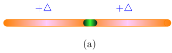
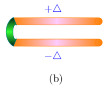
Figure 13: (Color online) Superconducting systems with (a) the same value of $\Delta$ throughout, and (b) the sign of $\Delta$ changing near one point shown in green (dark shade). There is also an impurity present at that point.

The impurity inside the SC that we have studied in Sec. VI corresponds to an arbitrary point in Fig. 13 (a) and to the region where $\Delta$ changes sign in Fig. 13 (b); both these points are shown in green (dark shade). The strength of the impurity $\lambda$ can be controlled by placing a gate near those points and varying the gate voltage.

Finally, the ends of the SC can be connected to NM leads through tunnel barriers. As discussed in Sec. II, these barriers can be characterized by their strength $\lambda$.

In Secs. II-IV, we discussed a conductance $G_{C}$ in which pairs of electrons can appear in (or disappear from) the $p$-wave SC. At a microscopic level we can understand these processes as occurring due to a Cooper pair going from the $s$-wave SC to the $p$-wave SC (or vice versa). Finally we have to assume that the two NM leads and the $s$-wave SC form a closed electrical circuit so that we can measure the conductances $G_{N}$ and $G_{C}$.

We would like to note here that some other realizations of systems in which the pairing $\Delta$ changes sign at one point have been discussed before alicea1 ; kesel ; ojanen ; lucig ; klino3 . However the effect of an impurity at that point and the conductances of the system were not studied in these papers. Although the geometry of the system discussed in Ref. kesel, looks similar to ours (Fig. 13 (b)), the details are quite different. The set-up proposed in Ref. kesel, requires proximity to two different $s$-wave superconductors and also requires a superconducting loop threaded by a magnetic flux equal to $hc/4e$.

VIII Conclusions

In this paper, we have studied the Majorana modes and conductances of a one-dimensional system consisting of a $p$-wave SC of length $L$ connected by tunnel barriers to two NM leads. We have considered two cases:  (i) the $p$-wave $\Delta$ pairing has the same sign everywhere in the SC (with, possibly, an impurity potential with strength $\lambda$ present at one point inside the SC), and (ii) $\Delta$ changes sign at one point in the SC (and an impurity present there). We have used a continuum model to derive the boundary conditions at the junctions between the SC and the NM. Using these conditions, we have numerically studied two conductances, $G_{N}$ (from one lead to the other) and the Cooper pair conductance $G_{C}$ (from one lead to the SC), when the energy $E$ of an electron incident from one of the leads lies within the SC gap.

We have studied three ranges of values of $L$ with respect to the length $\eta$ (the length scale associated with the SC gap). We find a rich pattern of variations of the conductances as functions of $L$ and $E$. We have provided analytical explanations for these behaviors by studying some special limits, such as the Majorana modes at the ends of a SC box with no leads, and the conductances of the NSN system in the limit when the tunnel barriers $\lambda$ between the SC and the leads are very large. In this limit, we find that there are quantization conditions for the length $L$ at which $G_{N}$ and $G_{C}$ have peaks. We find that the presence of Majorana modes at the ends of the SC has a significant effect on the conductances; the latter have peaks exactly at the energies of the Majorana modes. We do not find any noticeable difference between the behaviors of the conductances for the cases of uniform $\Delta$ versus $\Delta$ changing sign at one point in the SC, although the latter system has two additional Majorana modes at that point. This implies that the presence of Majorana modes inside the SC (i.e., far away from the leads) has no major effect on the conductances.

[We would like to mention here that the hybridization of the Majorana modes at the ends of the wire can also occur due to tunneling processes involving virtual quasiparticle states in the bulk $s$-wave SC which is in proximity to the wire zyuzin . This can give rise to an energy splitting even if the Majorana modes cannot directly hybridize through the wire. A discussion of this effect is beyond the scope of our model].

For the case that $\Delta$ changes sign at one point in the SC, we have used a lattice model to study the Majorana modes which occur near that point. We find that these modes have a noticeable effect on the local particle density as a function of the Fermi energy. Further, these modes are very robust in that they stay at zero energy even if we vary the potential near that point. This is because a symmetry of the system prevents these modes from hybridizing with each other.

Next, we have studied the effect of interactions between the electrons in a SC. Using bosonization, we have studied the RG flows of the different parameters of the theory such as the pairing $\Delta$ and the strength $\lambda$ of an impurity potential which may be present either inside the SC or at the junctions of the SC and the leads as tunnel barriers. For repulsive interactions, the Luttinger parameter $K<1$; we then find that $\Delta$ decreases while $\lambda$ increases as the length scale increases. We studied the effect of this on the Majorana modes and on the conductances. In particular, we find that if an impurity is present inside the SC, it can grow and eventually cut the SC into two parts if $L$ is large enough; then two Majorana modes can appear near the impurity. This is in contrast to the case where $\Delta$ changes sign at one point and there is also an impurity present there. We then find that there are always two Majorana modes near that point regardless of how small or large the impurity strength is.

Finally, we have discussed some experimental implementations of our model. We have shown that the cases of both uniform $\Delta$ and $\Delta$ changing at one point can be realized. The second case is interesting because two Majorana modes are expected to appear near that point. We have shown that these additional modes have no noticeable effect on the conductances of the system; this may be because we have considered a configuration in which the NM leads lie far away from these modes. It should be possible to study these modes by attaching a lead at that point and measuring the conductance in that lead zhou ; weit . Another way to detect these modes would be through STM studies of the local particle density as a function of energy.

References

- (1)
- (2) M. Z. Hasan and C. L. Kane, Rev. Mod. Phys. 82, 3045 (2010).
- (3) X.-L. Qi and S.-C. Zhang, Rev. Mod. Phys. 83, 1057 (2011).
- (4) A. Kitaev, Physics-Uspekhi 44, 131 (2001).
- (5) R. M. Lutchyn, J. D. Sau, and S. Das Sarma, Phys. Rev. Lett. 105, 077001 (2010).
- (6) Y. Oreg, G. Refael, and F. von Oppen, Phys. Rev. Lett. 105, 177002 (2010).
- (7) A. C. Potter and P. A. Lee, Phys. Rev. Lett. 105, 227003 (2010).
- (8) V. Shivamoggi, G. Refael, and J. E. Moore. Phys. Rev. B 82, 041405(R) (2010).
- (9) D. Sen and S. Vishveshwara, EPL 91, 66009 (2010).
- (10) L. Fidkowski and A. Kitaev, Phys. Rev. B 83, 075103 (2011).
- (11) P. W. Brouwer, M. Duckheim, A. Romito, and F. von Oppen, Phys. Rev. Lett. 107, 196804 (2011), and Phys. Rev. B 84, 144526 (2011).
- (12) J. Alicea, Y. Oreg, G. Refael, F. von Oppen, and M. P. A. Fisher, Nature Phys. 7, 412 (2011).
- (13) I. C. Fulga, F. Hassler, A. R. Akhmerov, and C. W. J. Beenakker, Phys. Rev. B 83, 155429 (2011).
- (14) K. T. Law and P. A. Lee, Phys. Rev. B 84, 081304(R) (2011).
- (15) T. D. Stanescu, R. M. Lutchyn, and S. Das Sarma, Phys. Rev. B 84, 144522 (2011).
- (16) S. Gangadharaiah, B. Braunecker, P. Simon, and D. Loss, Phys. Rev. Lett. 107, 036801 (2011).
- (17) E. M. Stoudenmire, J. Alicea, O. A. Starykh, and M. P. A. Fisher, Phys. Rev. B 84, 014503 (2011).
- (18) S. B. Chung, H.-J. Zhang, X.-L. Qi, and S.-C. Zhang, Phys. Rev. B 84, 060510 (2011).
- (19) E. Sela, A. Altland, and A. Rosch, Phys. Rev. B 84, 085114 (2011).
- (20) R. M. Lutchyn and M. P. A. Fisher, Phys. Rev. B 84, 214528 (2011).
- (21) A. R. Akhmerov, J. P. Dahlhaus, F. Hassler, M. Wimmer, and C. W. J. Beenakker, Phys. Rev. Lett. 106, 057001 (2011).
- (22) W. DeGottardi, D. Sen, and S. Vishveshwara, New. J. Phys. 13, 065028 (2011).
- (23) L. Jiang, T. Kitagawa, J. Alicea, A. R. Akhmerov, D. Pekker, G. Refael, J. I. Cirac, E. Demler, M. D. Lukin, and P. Zoller, Phys. Rev. Lett. 106, 220402 (2011).
- (24) T. Dirks, T. L. Hughes, S. Lal, B. Uchoa, Y.-F. Chen, C. Chialvo, P. M. Goldbart, and N. Mason, Nature Phys. 7, 386 (2011).
- (25) L. Fidkowski, J. Alicea, N. H. Lindner, R. M. Lutchyn, and M. P. A. Fisher, Phys. Rev. B 85, 245121 (2012).
- (26) S. Tewari and J. D. Sau, Phys. Rev. Lett. 109, 150408 (2012).
- (27) M. Gibertini, F. Taddei, M. Polini, and R. Fazio, Phys. Rev. B 85, 144525 (2012).
- (28) J. S. Lim, L. Serra, R. López, and R. Aguado, Phys. Rev. B 86, 121103 (2012).
- (29) M. Tezuka and N. Kawakami, Phys. Rev. B 85, 140508(R) (2012).
- (30) R. Egger and K. Flensberg, Phys. Rev. B 85, 235462 (2012).
- (31) A. M. Lobos, R. M. Lutchyn, and S. Das Sarma, Phys. Rev. Lett. 109, 146403 (2012).
- (32) F. Pientka, G. Kells, A. Romito, P. W. Brouwer, and F. von Oppen, Phys. Rev. Lett. 109, 227006 (2012).
- (33) T. D. Stanescu, S. Tewari, J. D. Sau, and S. Das Sarma, Phys. Rev. Lett. 109, 266402 (2012).
- (34) D. Roy, C. J. Bolech, and N. Shah, Phys. Rev. B 86, 094503 (2012), and arXiv:1303.7036.
- (35) A. M. Cook, M. M. Vazifeh, and M. Franz, Phys. Rev. B 86, 155431 (2012).
- (36) F. L. Pedrocchi, S. Chesi, S. Gangadharaiah, and D. Loss, Phys. Rev. B 86, 205412 (2012).
- (37) D. Sticlet, C. Bena, and P. Simon, Phys. Rev. Lett. 108, 096802 (2012); D. Chevallier, D. Sticlet, P. Simon, and C. Bena, Phys. Rev. B 85, 235307 (2012).
- (38) I. Martin and A. F. Morpurgo, Phys. Rev. B 85, 144505 (2012).
- (39) P. San-Jose, E. Prada, and R. Aguado, Phys. Rev. Lett. 108, 257001 (2012); E. Prada, P. San-Jose, and R. Aguado, Phys. Rev. B 86, 180503 (2012).
- (40) J. Klinovaja and D. Loss, Phys. Rev. B 86, 085408 (2012).
- (41) J. Alicea, Rep. Prog. Phys. 75, 076501 (2012).
- (42) F. Hassler and D. Schuricht, New J. Phys. 14, 125018 (2012).
- (43) J. D. Sau and S. Das Sarma, Nature Communications 3, 964 (2012).
- (44) S. Das Sarma, J. D. Sau, and T. D. Stanescu, Phys. Rev. B 86, 220506(R) (2012).
- (45) J. D. Sau, C. H. Lin, H.-Y. Hui, and S. Das Sarma, Phys. Rev. Lett. 108, 067001 (2012).
- (46) J. Liu, A. C. Potter, K. T. Law, and P. A. Lee, Phys. Rev. Lett. 109, 267002 (2012).
- (47) L.-J. Lang and S. Chen, Phys. Rev. B 86, 205135 (2012).
- (48) Y. Niu, S. B. Chung, C.-H. Hsu, I. Mandal, S. Raghu, and S. Chakravarty, Phys. Rev. B 85, 035110 (2012).
- (49) M. Leijnse and K. Flensberg, Semicond. Sci. Technol. 27, 124003 (2012).
- (50) F. Pientka, A. Romito, M. Duckheim, Y. Oreg, and F. von Oppen, New J. Phys. 15, 025001 (2013).
- (51) D. Rainis, L. Trifunovic, J. Klinovaja, and D. Loss, Phys. Rev. B 87, 024515 (2013).
- (52) D. Chevallier, D. Sticlet, P. Simon, and C. Bena, Phys. Rev. B 87, 165414 (2013).
- (53) T. D. Stanescu and S. Tewari, J. Phys. Condens. Matter 25, 233201 (2013).
- (54) S. Nadj-Perge, I. K. Drozdov, B. A. Bernevig, and A. Yazdani, Phys. Rev. B 88, 020407(R) (2013).
- (55) W. DeGottardi, D. Sen, and S. Vishveshwara, Phys. Rev. Lett. 110, 146404 (2013).
- (56) W. DeGottardi, M. Thakurathi, S. Vishveshwara, and D. Sen, Phys. Rev. B 88, 165111 (2013).
- (57) X. Cai, L.-J. Lang, S. Chen, and Y. Wang, Phys. Rev. Lett. 110, 176403 (2013).
- (58) A. Keselman, L. Fu, A. Stern, and E. Berg, Phys. Rev. Lett. 111, 116402 (2013).
- (59) T. Ojanen, Phys. Rev. B 87, 100506(R) (2013).
- (60) P. Lucignano, F. Tafuri, and A. Tagliacozzo, Phys. Rev. B 88, 184512 (2013); Erratum, Phys. Rev. B 88, 219902 (2013).
- (61) C. W. J. Beenakker, Annu. Rev. Condens. Matter Phys. 4, 113 (2013).
- (62) I. Adagideli, M. Wimmer, and A. Teker, Phys. Rev. B 89, 144506 (2014).
- (63) T. D. Stanescu and S. Tewari, Phys. Rev. B 89, 220507(R) (2014).
- (64) E. Eriksson, C. Mora, A. Zazunov, and R. Egger, Phys. Rev. Lett. 113, 076404 (2014).
- (65) A. Manolescu, D. C. Marinescu, and T. D. Stanescu, J. Phys. Condens. Matter 26, 172203 (2014).
- (66) A. M. Lobos and S. Das Sarma, New J. Phys. 17, 065010 (2015).
- (67) O. Kashuba and C. Timm, Phys. Rev. Lett. 114, 116801 (2015).
- (68) M. Guigou, N. Sedlmayr, J. M. Aguiar-Hualde, and C. Bena, arXiv:1407.1393v2.
- (69) J. Klinovaja and D. Loss, Eur. Phys. J. B 88, 62 (2015).
- (70) R. Doornenbal, G. Skantzaris, and H. Stoof, arXiv:1408.5106v2.
- (71) H.-C. Kao, arXiv:1411.4393.
- (72) E. Dumitrescu, B. Roberts, S. Tewari, J. D. Sau, and S. Das Sarma, Phys. Rev. B 91, 094505 (2015).
- (73) E. Dumitrescu, G. Sharma, J. D. Sau, and S. Tewari, arXiv:1501.00985.
- (74) C. Spanslatt, E. Ardonne, J. C. Budich, and T. H. Hansson, arXiv:1501.03413.
- (75) S. Hegde, V. Shivamoggi, S. Vishveshwara, and D. Sen, New J. Phys. 17, 053036 (2015).
- (76) V. Mourik, K. Zuo, S. M. Frolov, S. R. Plissard, E. P. A. M. Bakkers, and L. P. Kouwenhoven, Science 336, 1003 (2012).
- (77) M. T. Deng, C. L. Yu, G. Y. Huang, M. Larsson, P. Caroff, and H. Q. Xu, Nano Lett. 12, 6414 (2012).
- (78) A. Das, Y. Ronen, Y. Most, Y. Oreg, M. Heiblum, and H. Shtrikman, Nature Phys. 8, 887 (2012).
- (79) A. D. K. Finck, D. J. Van Harlingen, P. K. Mohseni, K. Jung, and X. Li, Phys. Rev. Lett. 110, 126406 (2013).
- (80) E. J. H. Lee, X. Jiang, M. Houzet, R. Aguado, C. M. Lieber, and S. De Franceschi, Nature Nanotechnology 9, 79 (2014).
- (81) A. D. K. Finck, C. Kurter, Y. S. Hor, and D. J. Van Harlingen, Phys. Rev. X 4, 041022 (2014).
- (82) S. Nadj-Perge, I. K. Drozdov1, J. Li, H. Chen, S. Jeon, J. Seo, A. H. MacDonald, B. A. Bernevig, and A. Yazdani, Science 346, 602 (2014).
- (83) L. P. Rokhinson, X. Liu, and J. K. Furdyna, Nature Phys. 8, 795 (2012).
- (84) G. E. Blonder, M. Tinkham, and T. M. Klapwijk, Phys. Rev. B 25, 4515 (1982).
- (85) A. Kastalsky, A. W. Kleinsasser, L. H. Greene, R. Bhat, F. P. Milliken, and J. P. Harbison, Phys. Rev. Lett. 67, 3026 (1991).
- (86) C.-R. Hu, Phys. Rev. Lett. 72 1526 (1994); J. Yang and C.-R. Hu, Phys. Rev. B 50, 16766 (1994).
- (87) Y. Tanaka and S. Kashiwaya, Phys. Rev. Lett. 74, 3451 (1995).
- (88) K. Sengupta, I. Zutić, H.-J. Kwon, V. M. Yakovenko, and S. Das Sarma, Phys. Rev. B 63, 144531 (2001).
- (89) K. Sengupta, H.-J. Kwon, and V. M. Yakovenko, Phys. Rev. B 65, 104504 (2002).
- (90) H.-J. Kwon, K. Sengupta and V. M. Yakovenko, Eur. Phys. J. B 37, 349 (2004).
- (91) T. Yokoyama, Y. Tanaka, and J. Inoue, Phys. Rev. B 74, 035318 (2006).
- (92) T. Yokoyama, Y. Tanaka, and N. Nagaosa, Phys. Rev. Lett. 102, 166801 (2009).
- (93) A. Hayat, P. Zareapour, S. Y. F. Zhao, A. Jain, I. G. Savelyev, M. Blumin, Z. Xu, A. Yang, G. D. Gu, H. E. Ruda, S. Jia, R. J. Cava, A. M. Steinberg, and K. S. Burch, Phys. Rev. X 2, 041019 (2012).
- (94) K. T. Law, P. A. Lee, and T. K. Ng, Phys. Rev. Lett. 103, 237001 (2009).
- (95) A. Soori, O. Deb, K. Sengupta, and D. Sen, Phys. Rev. B 87, 245435 (2013).
- (96) A. F. Andreev, Sov. Phys. JETP 19, 1228 (1964).
- (97) M. Thakurathi, A. A. Patel, D. Sen, and A. Dutta, Phys. Rev. B 88, 155133 (2013).
- (98) A. O. Gogolin, A. A. Nersesyan, and A. M. Tsvelik, Bosonization and Strongly Correlated Systems (Cambridge University Press, Cambridge, 1998).
- (99) J. von Delft and H. Schoeller, Ann. Phys. (Leipzig) 7, 225 (1998).
- (100) S. Rao and D. Sen, in Field theories in Condensed Matter Physics, edited by S. Rao (Hindustan Book Agency, New Delhi, 2001).
- (101) T. Giamarchi, Quantum Physics in One Dimension (Oxford University Press, Oxford, 2004).
- (102) A. A. Zyuzin, D. Rainis, J. Klinovaja, and D. Loss, Phys. Rev. Lett. 111, 056802 (2013).
- (103) Y. Zhou and M. W. Wu, J. Phys. Condens. Matter 26, 065801 (2014).
- (104) L. Weithofer, P. Recher, and T. L. Schmidt, Phys. Rev. B 90, 205416 (2014).