Relaxors, spin-, Stoner- and cluster-glasses

Abstract

It is argued that the main characteristic features of displacive relaxor ferrolectrics of the form ${\rm{A(B,B^{\prime})}\rm{O}}_{3}$ with isovalent ${\rm{B,B^{\prime}}}$ can be explained and understood in terms of a soft-pseudospin analogue of conventional spin glasses as extended to itinerant magnet systems. The emphasis is on conceptual comprehension and on stimulating new perspectives with respect to previous and future studies. Some suggestions are made for further studies both on actual real systems and on test model systems to probe further. The case of heterovalent systems is also considered briefly.

1 Introduction

There has been much interest in relaxor ferroelectrics since their discovery in the 1950s by the group of George Smolenskii in the USSR [1], following interest in pure displacive ferroelectrics of perovskite structure and make-up ${AB\rm{O}}_{3}$, where $A$ is an ion of nominal charge +2, $B$ an ion of charge +4 and O is oxygen, of charge -2. In particular, a new class of alloy materials was discovered in $\mathrm{Pb(Mg}_{1/3}\mathrm{Nb}_{2/3}\mathrm{)O}_{3}$ (PMN) with interesting frequency-dependent peaks in its dielectric susceptibilities as a function of temperature [2], just below room temperature, but without any macroscopic polarization in the absence of applied fields. It has further turned out that there are manifestations of nano-scale polar domains (polar nano-regions, PNRs) [3], beneath a higher ‘Burns’ temperature [4] at which deviations from high-temperature paraelectricity become apparent, and non-ergodicity onsets beneath a temperature comparable with that of the susceptibility peaks [5], [6], [7]. However, more than half a century later than the discovery of these systems, there remains a lack of full understanding and agreement on the microscopic physical origin of the observed effects.

Recently, the present author proposed [8, 9] that a conceptual explanation may be found in analogy with a soft-spin variant of a conventional spin glass [10, 11, 12], with the glassy onset of non-ergodicity without global lattice change the analogue of a spin glass transition and the PNRs manifestations of localized state precursors of macroscopic order [13, 14], especially simply for a more recently discovered class of isovalent relaxors, such as $\mathrm{Ba(Zr}_{1-x}\mathrm{Ti}_{x})\mathrm{O}_{3}$ (BZT) in which the B-site ions are occupied randomly by Ti or Zr ions, both of charge +4. BZT is conceptually clearer than heterovalent PMN in which the +4 Ti-ions of $\mathrm{PbTi}\mathrm{O}_{3}$ are replaced randomly by a mixture of one third Mg +2 and two thirds Nb +5, giving rise also to significant effective random fields relative to the charge distribution of the underlying ${AB\rm{O}}_{3}$ perovskite template .

The author’s paper on BZT [8] was based on the premise that the key features of the relaxor behaviour of BZT can be understood by analogy with experimental spin glasses, as a compromise between frustrated intersite interactions and quenched site-to-site variations in the extent to which local displacements have propensities in the absence of interactions towards retaining their high-temperature perovskite structure or moving away from these positions. In addition, the strength of the binding needs to be sufficient to overcome the local displacive energy cost. More specifically it was argued that for displacive relaxors the glassy ordering is analogous to earlier proposals for itinerant glassy magnets such as RhCo [15], essentially a combination of the Stoner-glass concept introduced in [16] and a cluster glass with the PNRs analogues of the statistically cluster-localized moments proposed in [13, 14].

[8] was stimulated in part by a prior computer simulation study of BZT [17] for the 50/50 concentration case, with observations in that computer study explainable by theoretical modelling and analogy. The simulational studies observed both PNRs and ergodicity-breaking. The prediction in [8] that PNRs above the relaxor onset temperature (the low-frequency susceptibility peak temperature) but beneath a higher temperature can be viewed as statistically clustered localized phonons was given posterior support in experimental observations of [18].

However, not all researchers in the topic share the author’s vision and prefer other pictures, such as random fields as the driving mechanism [5, 19], even for the isovalent relaxors [20]. Also, the non-observation, at least to date, of relaxor behaviour in $\mathrm{Pb(Zr}_{1-x}\mathrm{Ti}_{x})\mathrm{O}_{3}$ has been suggested as a counter-example to the spin-glass analogy for an isovalent alloy [21, 22].

Hence, in this communication the author attempts to explain further his reasoning, indicating also some of the similarities and overlaps of his modelling with other descriptions, as well as some of the the differences, in the hope of clarifying the potential conceptual issues. The mathematical models discussed below are similar to those used by previous authors concerned with first-principles quantum-mechanical evaluation of effective classical Hamiltonians followed by computer simulation of their statistical mechanics [23, 17, 24]. However, the approach used below is complementary; minimalist and qualitative, using simplified Hamiltonians, approximations and analogies, with the aim of probing possibilities for understanding and suggesting opportunities for the incorporation of unconventional concepts in future thinking, experimentation and simulation, rather than concerned with precision or quantification.

2 Microscopic ‘moments’

In ferroelectrics (and antiferroelectrics and relaxors) systems are often classified as ‘order-disorder’ or as ‘displacive’, depending upon whether the macroscopic ordering is of discrete or continuous variables. For example, $\mathrm{NaN0}_{2}$ is considered as an order-disorder system since well-defined (discrete) local dipolar moments exist already above the ferroelectric ordering temperature, while $\mathrm{Ba}\mathrm{Ti}\mathrm{O}_{3}$ is usually described as a displacive ferroelectric since, to a first approximation, there is no local electric moment above the ferroelectric transition temperature but rather it grows continuously from zero as the temperature is reduced through the transition.

Correspondingly for magnetic systems one has (i) order-disorder transitions where the local magnetism is due to well-defined local moments, typically associated with incomplete d- and f-shell atoms or ions, (ii) an analogue of displacive transitions in (metallic) itinerant magnets where the magnetism is due to Coulombic interactions in conduction-electron bands, typically in d-electron metals, displacing the symmetry of up and down conduction bands.

Although order-disorder and displacive transitions are often viewed as separate entities, in fact they can be considered as continuously related through variation of suitable parameters. Thus, if the non-interacting local displacement contribution to a Hamiltonian takes the form

$$H_{L}=\kappa u^{2}+\lambda u^{4}$$ (1)

with $\lambda$ positive, then its minimum will be at $u=0$ for $\kappa$ positive but for $\kappa$ negative it has two minima at $u=\pm(-\kappa/2\lambda)^{1/2}$ . When site-to-site interaction effects are included, permitting a cooperative ordering, $\kappa$ positive corresponds to a ‘displacive’ transition, whereas $\kappa$ negative corresponds to ‘order-disorder’. The order-disorder case sharpens as the limits ($\kappa\to-\infty$, $\lambda\to\infty$, with $(\kappa/\lambda)\to$ const) are taken . Clearly, as $\kappa$ is taken through 0 one passes continuously between ‘order-disorder’ and ‘displacive’. This explains why experimentally some systems undergo phase transitions with a mixture of order-disorder and displacive aspects, as corresponding to small negative $\kappa$.

As an example of the ‘displacive’ modelling of an itinerant magnet, pure or alloy, one can consider the procedure described in [13, 14]. With some simplifying assumptions one may start from the Hubbard model

$$H=\sum_{ij,\sigma}t_{ij}a_{i\sigma}^{\dagger}a_{j\sigma}-{\frac{1}{4}}\sum_{i}U_{i}{\textit{{S}}}_{i}.{\textit{{S}}}_{i},$$ (2)

where the $a,a^{\dagger}$ are site- and spin-labelled d-electron annihilation and creation operators, ${\bf{S}}_{i}=\sum_{s,s^{\prime}=\pm 1}a^{\dagger}_{is}{\bm{\sigma}}_{ss^{\prime}}a_{is^{\prime}}$, where ${\bm{\sigma}}_{ss^{\prime}}$ is the Pauli matrix, and allowance is made for different atom types with different Coulomb repulsions $U$. For simplicity below, discussion is restricted to just two types of atom, one with $U=0$ and one with a finite $U$. Expressing the partition function in terms of a Grassmann functional integral in $a,a^{*}$ fields, linearising in terms of single sites by utilising the inverse of completing the square [25, 26]

$$\exp(a^{2})={\pi^{-1/2}}\int dx\exp(-x^{2}-2ax),$$ (3)

via an effective local magnetization field, perturbation-expanding in the magnetization field by integrating out the electron variables and taking the static approximation, one obtains an effective magnetization Hamiltonian

$$H_{M}=\sum_{i}(U^{-1}-\chi_{ii})|{\textit{{M}}}_{i}|^{2}-\sum_{ij;i\neq j}\chi_{ij}{\textit{{M}}}_{i}.{\textit{{M}}}_{j}$$

$$-\sum_{ijkl;\alpha\beta\gamma\delta}\Pi^{\alpha\beta\gamma\delta}_{ijkl}M^{\alpha}_{i}M^{\beta}_{j}M^{\gamma}_{k}M^{\delta}_{l}+...$$ (4)

where ${\bf{M}}_{i}=U_{i}{\bf{m}}_{i}=U_{i}<a^{\dagger}_{is}{{{\boldsymbol{\sigma}}}}_{ss^{\prime}}a_{is^{\prime}}>$, the $\chi_{ij}$ and $\Pi_{ijkl}$ are the two-site susceptibilities and analogous four-site functions of the bare conduction-band structure, and the sums are over only sites with $U_{i}\neq 0$. The local terms in this expression are

$$H_{ML}=\sum_{i}(U^{-1}-\chi_{ii})|{\textit{{M}}}_{i}|^{2}-\sum_{i;\alpha\beta\gamma\delta}\Pi^{\alpha\beta\gamma\delta}_{iiii}M^{\alpha}_{i}M^{\beta}_{i}M^{\gamma}_{i}M^{\delta}_{i}+...,$$ (5)

again over only sites with $U\neq 0$, which is immediately recognisable as being of the form of Equation (1), with $\kappa\sim(U^{-1}-\chi_{ii})$ and $\lambda\sim-\Pi_{iiii}{{\color[rgb]{0,0,0}>0}}$. It immediately yields the standard Anderson mean-field criterion ($(1-U\chi_{ii})<0$) for a local moment on an isolated ion with $U\neq 0$ in a sea of ions with $U=0$ [27].

3 Interactions

To exhibit phase transitions a system needs interactions as well as the local terms. For the case of the Hubbard model example for itinerant magnets these have already been exhibited in the extra terms in Equation (4) compared with Equation (5). The simplest interaction term is

$$H_{MI}=\sum_{ij;i\neq j}\chi_{ij}{\textit{{M}}}_{i}.{\textit{{M}}}_{j}.$$ (6)

This gives the condition for itinerant ferromagnetism in a simple pure system (all sites with the same $U$) as

$$1-U\sum_{J}\chi_{ij}<0,$$ (7)

the well-known Stoner criterion.

For displacive ferroelectrics the microscopic origin of terms like Equation (7) is different but the consequence is similar. Interactions occur both because of shortish-range quantum mechanical reasons, estimable by first principles density functional methods, and because of longer-range Coulombic interactions [30]. Restricting to two-site interactions and ignoring coupling to overall strains, these interaction terms may be subsumed to give the Hamiltonian schematically as

$$\begin{split}H_{DF}=\sum_{i}\{\kappa_{i}|\textit{{u}}_{i}|^{2}+\lambda_{i}|\textit{{u}}_{i}|^{4}+\gamma_{i}[u_{ix}^{2}u_{iy}^{2}+u_{iy}^{2}u_{iz}^{2}+u_{iz}^{2}u_{ix}^{2}]\}\\ +{{1/2}\sum_{(i,j;i\neq j)}H_{int}({\textit{{u}}}_{i},{\textit{{u}}}_{j},{\textit{{{R}}}}_{ij})}.\end{split}$$ (8)

To attain cooperative order in a system with positive $\kappa$ there needs to be a sufficient lowering of the free energy due to the interaction to overcome the local displacement penalty. This is the direct analogue of the condition for magnetic order given in the itinerant magnetic example above.

Thus, viewed this way, there is conceptual similarity between itinerant magnets and displacive ferroelectrics, a similarity that extends to more complex order, such as antiferroelectricity and charge-density-wave magnetism, if the the form of the interaction is such that (free) energy is lowest for such ordering. Both require a minimum interaction binding energy gain relative to the harmonic displacement energy cost in order to bootstrap cooperative order. In both itinerant magnetic and displacive electric cases there are well-known examples of pure systems which satisfy this requirement and others which do not; thus $\mathrm{Ba}\mathrm{Ti}\mathrm{O}_{3}$ is a ferroelectric at low enough temperature while $\mathrm{Ba}\mathrm{Zr}\mathrm{O}_{3}$ remains paraelectric at all temperatures (presumably because its $\kappa$ is too large), and analagously Co is a ferromagnet while pure Pd is only paramagnetic.

In displacive systems there are also couplings to the overall strain. These are relevant for systems with periodic ordering, such as ferroelectricity, permitting also changes in $c/a$ ratios, but are not so important in relaxor systems where the overall symmetry is not affected. Hence they are ignored in the main discussion here.

4 Alloys

The interest of this article is principally in alloys which exhibit glassiness, a broad range of timescales extending to very slow. This is evident in relaxor systems in the fact that the peaks in the susceptibility are significantly frequency-dependent, their temperatures increasing with frequency. This is in contrast to conventional transitions, such as that to ferroelectricity, where the susceptibility peak positions are little affected by the frequency of the probe.

Small amounts of alloying, randomly replacing host atoms by other elements, retain the main characteristics of the pure system transition, such as the independence of the susceptibility peak on frequency. Larger amounts of admixture in systems with frustration can (and, it is argued here, often do) lead to a relaxor (glass) state.

As was pointed out in [8], in analogy with well-known behaviour in conventional (local moment) spin glasses, the combination of frustrated interactions and locally variable $\kappa$ provide ingredients known to lead to spin glass behaviour, particularly when one of the constituents is essentially immobile, having a $\kappa$ that is too large (positive) to permit periodic ordering as a pure material.

Canonical experimental local moment spin glasses, such as AuFe, in which one ingredient is magnetic (here Fe) and the other non-magnetic (here Au) have Hamiltonians of the form

$$H_{SG}=-{1/2}\sum_{(i,j;i\neq j)(Mag)}{J}({\textit{{R}}}_{ij}){\textit{{S}}}_{i}.{\textit{{S}}}_{j}$$ (9)

where the ${\it\bf{S}}_{i}$ are localised spins on the magnetic atoms and the summation is restricted to the corresponding sites. The exchange interaction ${J}({\textit{{R}}}_{ij})$ is frustrated; in the case of a simple metallic system like AuFe as the RKKY form $J{\cos(2k_{F}(R))}/R^{3}$, which provides spatial frustration through its oscillations in sign; while in insulating spin glasses in some cases the range of interaction is shorter but still spatially frustrated through antiferromagnetic terms beyond nearest neighbour, as, for example, in ${\textrm{Eu}}_{x}{\textrm{Sr}}_{(1-x)}{\textrm{S}}$, and in others there is frustration of long-range dipolar character, for example in ${\textrm{LiHo}}_{x}{\textrm{Y}}_{(1-x)}{\textrm{F}}_{4}$ .

Let us next consider displacive alloys ${A(B^{\prime},B^{\prime})}O_{3}$ in which the $B^{\prime}$, $B^{\prime\prime}$ are isovalent (both 4+) and, for concise simplicity, assume that the effects of the $A$ and $O$ ions are absorbed into an effective interaction between the $B$ ions. Each of the $B$-types has its own value of $\kappa$. If one of them (say that of $B^{\prime}$) is sufficiently large such that when it is the only $B$-constituent the material is paraelectric at all temperatures, then its displacements can be ignored and the Hamiltonian can be written as a sum over only the other $B$-sites ($B^{\prime\prime}$)

$$H_{DR}=\sum_{i}\{\kappa_{i}|\textit{{u}}_{i}|^{2}+\lambda_{i}|\textit{{u}}|^{4}\}+{{1/2}\sum_{i,j;i\neq j}H_{int}^{Beff}({\textit{{u}}}_{i},{\textit{{u}}}_{j},{\textit{{R}}}_{ij})}$$ (10)

where the summations are now over $B^{\prime\prime}$-sites only . Global strain coupling is ignored here since it has been observed that the average cubic perovskite structure is maintained in transitions from paraelectric to relaxor . In the case of BZT the summations are thus only over Ti sites. The interaction term $H_{int}^{Beff}({\textit{{u}}}_{i},{\textit{{u}}}_{j},{\textit{{R}}}_{ij)}$ is spatially frustrated but for the pure Ti case the minimum of $H_{DR}$ is ferroelectric.

To second order in the displacements the interaction term may be expressed in the form

$$H_{int}({\textit{{u}}}_{i},{\textit{{u}}}_{j},{\textit{{R}}}_{ij})=-{1/2}\sum_{(i,j;i\neq j;\alpha,\beta)}J_{\alpha\beta}({\textbf{R}}_{ij})u_{i,\alpha}u_{j,\beta}$$ (11)

where $J_{\alpha\beta}({\textbf{R}}_{ij})$ is made up of terms of shortish range but extending beyond nearest neighbour, calculable by first-principles quantum analysis, and others of long-ranged dipolar character [23]. Both involve frustration with terms of opposing character. Given the evidence from magnetic spin glasses that many types of frustration can lead to a spin glass state in the presence of sufficient quenched disorder, it seems reasonable to expect that a similar situation can occur in displacive ferroelectrics if their fundamental interactions are frustrated, there is sufficient quenched disorder such that the potential binding energy gain is greatest for a distorted state without periodic order, and the potential binding energy of spontaneous distorsion is sufficient to overcome the local displacement energy costs. This expectation for BZT is in accord the simulations of Akbarzadeh et. al [17] on BZT 50/50, showing the characteristic spin glass signature of a separation between field cooled (FC) and zero-field cooled (ZFC) quasi-static susceptibilities beneath a critical temperature, and the experiments of several groups [28, 29] showing significant frequency-dependence in peaking of the finite-frequency susceptibilities.

In comparison one might note that for the itinerant alloy system also, the interaction term $\chi_{ij}$ is spatially frustrated, in the same Fermi-surface-driven manner as the RKKY interaction.

5 Mean field theory, free energy, polar nanoregions, localization and phase transitions

In this section we consider mean field solutions for displacive alloys. Because of the spatial disorder in Equation (10) mean field theory must allow for spatial variations in $<{\bf{u_{i}}}>$. For zero temperature one can minimize $H_{DR}$, but for finite temperature one should minimise the corresponding free energy, which we shall write as

$$F_{DR}=\sum_{i}\{\tilde{\kappa}_{i}(T)|\textit{{u}}_{i}|^{2}+\tilde{\lambda}_{i}(T)|\textit{{u}}|^{4}\}+{\sum_{ij...}^{\prime}F_{int}({\textit{{u}}}_{i},{\textit{{u}}}_{j},...{\textit{{R}}}_{ij...})}$$ (12)

and, for simplicity, further concentrate on bi-linear contributions to $F_{int}$ and scalar $u$;

$$F_{SDR}=\sum_{i}\{\tilde{\kappa}_{i}(T)u_{i}^{2}+\tilde{\lambda}_{i}(T)u_{i}^{4}\}-{{1/2}\sum_{i,j;i\neq j}\tilde{J}(R_{ij},T)u_{i}u_{j}}.$$ (13)

All the coefficients are temperature-dependent, but the most important for our purpose is $\tilde{\kappa}_{i}$ which is expected to increase with temperature, making bootstrapping order more difficult as temperature is increased and yielding paraelectricity as the high temperature phase. It is assumed that $\tilde{\lambda}$ remains positive throughout . Again for simplicity, the temperature dependence of $\tilde{\lambda}$ and $\tilde{J}$ (or $F_{int}$) will be suppressed in the discussion.

Minimizing $F_{SDR}$, Equation (12), with respect to the $\{u_{i}\}$ yields

$$-2\tilde{\kappa}_{i}(T)u_{i}+{\sum_{j}\tilde{J}(R_{ij})u_{j}}=4\tilde{\lambda}_{i}u_{i}^{3}.$$ (14)

Clearly, this equation always allows solutions $\{{u=0}\}$, corresponding to undisplaced paraelectricity, but interest is in possible solutions $\{{u\neq 0}\}$. Such $\{{u\neq 0}\}$ solutions only occur for small enough $\{\tilde{\kappa}\}$ such that the $\tilde{J}$ term can bootstrap-yield a right hand side (r.h.s.) of Equation (14) that has the same sign as $u_{i}$. They can be either extended or localized, depending upon whether $\{u\neq 0\}$ sites span the whole system or not. Localized states correspond to PNRs while a true phase transition requires a globally extended solution.

A potentially helpful way to understand these possibilities is to compare Equation (14) with the Anderson (eigenfunction) localization equation [31]

$$\epsilon_{i}\phi_{i}+{\sum_{j}t_{ij}\phi_{i}}=E\phi_{i},$$ (15)

with the identifications

$$\epsilon_{i}=-\tilde{\kappa_{i}}(T);\hskip 28.45274ptt_{ij}={\tilde{J}}(R_{ij})/2,$$ (16)

corresponding to diagonalization of the r.h.s. of Equation (14). This shows that that the condition for non-zero solutions to Equation (14) corresponds to that for $E\geq 0$ solutions to Equation (15). Thus, if $E<0$ the system remains paraelectric with all $u_{i}=0$.

The density of states $\rho(E)$ of solutions of Equation (15) of eigenvalue $E$ gives insight into the corresponding solutions of Equation (14). Figure 1 shows a schematic density of states for a system such as described by Equation (15), for a situation with all eigenvalues negative, corresponding for Equation (14) to a temperature too high for $u\neq 0$ solutions, in the paraelectric region. As the temperature is reduced the density of states distribution moves to higher $E$. At a first characteristic temperature the density of states crosses zero and permits non-zero $u$ solutions to Equation (14).

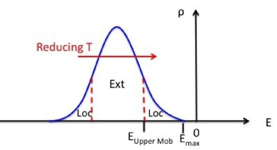
Figure 1: Schematic density of states of an analogous Anderson model, showing typical localized (Loc) and extended (Ext) states in the case of a disordered system. Also shown is the effect of reducing temperature in the displacive system. Polar nanoregions onset when the upper band edge ($\textrm{E}_{\textrm{max}}$) crosses zero energy and macroscopic order occurs when the upper mobility edge ($\textrm{E}_{\textrm{{Upper Mob}}}$) crosses zero.

For a pure system the eigenfunction of Equation (15) with the largest eigenvalue is extended . Thus, with a small enough $\kappa$ there will be a spontaneous phase transition when the highest eigenvalue reaches zero, to a phase with the symmetry of the highest eigenfunction. As the temperature is lowered the order parameter of the symmetry breaking will initially grow linearly in ${(E_{c})}^{1/2}$ or equivalently${(T_{c}-T)^{1/2}}$. $\mathrm{Ba}\mathrm{Ti}\mathrm{O}_{3}$ (BT) is an example (with the transition to a ferroelectric).

However, in a disordered system the states near the band edges of Equation (15) are localized, with extended states only possible within ‘mobility edges’ (see Figure(1). Thus, in a disordered system, as the temperature is reduced there first onset metastable localized clusters at a temperature $T_{A}$ at which the upper band edge of the Anderson equation reaches zero energy, with a possible true phase transition only at a lower temperature $T_{c}$ at which an extended state becomes a solution to Equation (14), analogous to where the upper mobility edge of the Anderson model crosses zero.

In conventional Anderson localization modelling the $t_{ij}$ are unfrustrated and usually short-ranged and the extended states have the average symmetry of the pure system. In the present problem, however, the $t_{ij}$ are frustrated as a function of separation. This allows for the largest interactive binding energy compared with the local displacement cost to be for an unconventional order, as is the case for spin glasses with good local moments in the presence of a sufficient combination of quenched disorder and frustration. Thus, for a displacive system, depending upon the level of disorder and frustration, the true phase transition can be to (i) a phase that is periodically ordered on average or (ii) to a spin glass-like phase with $p=\overline{\langle u\rangle}=0$ but $q=\overline{{\langle u\rangle}^{2}}\neq 0$ or (iii) there can be no cooperative order at all. This is in accord with observations on $\mathrm{Ba(Zr}_{1-x}\mathrm{Ti}_{x})\mathrm{O}$ [28, 37] where the interaction term is spatially frustrated but the pure $x=1$ system is ferroelectric, that the ordering is found to be ferroelectric for $x\geq 0.75$, but for $0.65\geq x\geq 0.25$ the ordering is as a relaxor. The absence of any ordered phase for $x\leq 0.25$ suggests that, for this concentration range, the upper mobility edge is not reached as $T\to 0$ and there is no true phase transition, as as is the situation in pure $\mathrm{Ba}\mathrm{Zr}\mathrm{O}_{3}$ (BZ). Precursor localized displaced nanoregions are expected for $0<x<1$.

Note that it is not proven here that the intermediate concentration phase will be a pseudo-spin glass but it is strongly suggested as a reasonable possibility given (i) the similarity of Equation (9) and Equations (10) and (13) and (ii) the fact that interactions in relaxor systems are frustrated by long-range Coulomb/dipolar interactions as well as short range interactions and (iii) magnetic systems have provided ample evidence of the existence of spin glasses for a number of different types of frustrated interaction and quenched disorder.

By comparison with the case of spin glass systems, the paraelectric-to-ferroelectric transitions are expected to be sharp, with little dependence on probe frequency or history-dependence, whereas relaxor transitions (c.f. spin glass) are expected to be sluggish with significant probe-frequency-dependence and history-dependence (as observable in a separation of FC and ZFC static susceptibilities [32, 7]).

The glassiness and its consequence on history-dependence of conventional spin glasses can be studied within a more sophisticated mean field theory in terms of the recognition of the existence of many ‘pure states’ and the identification of the (low-field limit) FC and ZFC susceptibilities in terms of different ‘overlap’ contributions [33]. For example, for the SK $\pm 1$ Ising spin glass,

$$\chi^{FC}=T^{-1}(1-\int_{0}^{1}dxq(x));\hskip 14.22636pt\chi^{ZFC}=T^{-1}(1-q(x=1))$$ (17)

where

$$dx/dq=P(q)=\sum_{S,S^{\prime}}\delta(q-q_{S,S^{\prime}});\hskip 14.22636ptq_{S,S^{\prime}}=N^{-1}\sum_{i}<\sigma_{i}>_{S}<\sigma_{i}>_{S^{\prime}}$$ (18)

and the $S,S^{\prime}$ are pure states; $q_{S,S^{\prime}}$ is known as the overlap between the pure states $S$ and $S^{\prime}$. The existence of a non-trivial distribution of pure states implies glassy dynamics and can be related to the dynamical breakdown of conventional equilibrium statistical mechanical connections between fluctuations and dissipation (see e.g. [34]). It also leads to the concept of a hierarchy of timescales [35] and hence a severe frequency-dependence of peaks in the susceptibility [36]. However, the reader is referred to the extensive spin glass literature for further details.

Note that the higher energy localized states of the Anderson model with the parameter identification of eqn. (16) correspond to statistically clustered regions with higher than average Ti concentration (sites with higher $\epsilon$) and that, following BT, internally they will have dominantly $\phi$ of the same sign, so that the corresponding regions for eqn. (14) will have a tendency towards internal ferroelectric ordering, hence polar nano-regions.

Turning now to the localized states above the upper mobility edge of the Anderson analogue, it is tempting to approximate by

$$u_{i}=0;\hskip 2.84544ptE<0,\hskip 14.22636pt|u_{i}|\approx\{E/[2\tilde{\lambda}]\}^{1/2}{\rm{on}}\hskip 2.84544pt{\rm{sites}}\hskip 2.84544pt{\rm{with}}\hskip 2.84544pt{\rm{eigenstate}}\hskip 2.84544pt\phi_{i}\neq 0;\hskip 2.84544ptE>0,$$ (19)

However, in fact account must be taken of the polarizations associated with condensation of higher E eigenfunctions in assessing the potential for condensation of local polarizations associated with lower E. In a pure system, where the eigenstates are extended, this normally results in suppression of the ordering associated with the lower eigenstates. In the case of localized eigenstates however there exists the possibility that there may still remain the many separated localized polarization clusters, with effective interactions between them that are too weak to cause coalescence to an extended state above a characteristic temperature, at which there can be a transition to a phase which may be either periodic on average or relaxor, depending upon the energetic balance. Explicit solution of Equation (14), or a simplification - see the next section - would be valuable to assess this further within the context of mean field theory, but the observation of PNRs in both experiment and simulation appear to demonstrate that such localized states do exist at intermediate temperatures, while the observation of the onset of non-ergodicity at a lower temperature suggests the relaxor interpretation as a pseudo-softspin glass.

PNRs will contribute to deviations from pure paraelectricity, so it is tempting to identify $T_{A}$ with the Burns temperature $T_{B}$. Caution is needed in a precise identification of the temperatures, not only because the theory discussed is only for static equilibrium and even then in mean field theory, but also in the absence of detailed investigation of the form of the density of states near the band edges and the weightings of localized states to the susceptibility. However, it seems probable that $T_{B}$ measures the temperature region where the mean field localized states start to have sufficient weight to contribute significantly and the conceptualization provides a useful starting point for further theoretical modelling and further simulational investigation, beyond that in [17, 24]. It is also notable that the Burns temperature in BZT is comparable with the ferroelectric transition temperature in BT, which is likely to be close to where the upper limit of the Anderson density of states crosses zero.

Note that this simple picture already provides for the three characteristic features attributed to a displacive relaxor [20]; (i) significant frequency-dependence of the temperature of peaking of the susceptibility, with higher frequencies peaking at higher temperatures, (ii) absence of overall global spontaneous polarization or other structural symmetry-breaking and (iii) longish-lived polar nanoclusters beneath a higher temperature.

Although BZT has been taken as an example, the picture presented here can be applied to other isovalent relaxor systems, such as $\mathrm{Ba(Sn}_{1-x}\mathrm{Ti}_{x})\mathrm{O}_{3}$ (BST) [20]. Indeed, the observation that the critical concentration $x$ for crossover from ferroelectric to relaxor is very similar in BZT and BST is in accord with the expectation that both Zr and Sn are effectively immobile since the ionic radii of Zr 4+ (86 pm) and Sn 4+ (83 pm) are almost identical and significantly larger than (mobile) Ti 4+ (74.5 pm) [38].

6 Random site to random bond

Above we have concentrated on random site-occupation. In the conventional local moment spin glass model, Equation (9), the summation is over only the magnetic sites. In the case of a displacive ferroelectric/relaxor with one of the constituents having a $\kappa$ too large to allow order when pure, such as Zr in BZT, then in the corresponding Equation (10) one can restrict the summmation to the potentially ordering sites, Ti in the case of BZT. One can then rewrite the relevant Hamiltonians in terms of the potentially ordering ions only by relabelling the latter as $\{k,l\}$ to yield random bond forms, summed on all (new) sites. Thus for the spin glass system

$$H_{RBSG}=-\sum_{(kl)}{J}_{kl}{\textit{{S}}}_{k}.{\textit{{S}}}_{l}$$ (20)

and for the relaxor system

$$H_{RBDR}=\sum_{k}\{\kappa|\textit{{u}}_{k}|^{2}+\lambda|\textit{{u}}_{k}|^{4}\}+{\sum_{k>l}J_{kl}{\textit{{u}}}_{k}{\textit{{u}}}_{l}},$$ (21)

where the $J_{kl}$ are now quasi-random, actually determined by the $\{J_{i_{k}j_{l}}\}$ where $i_{k}$, $j_{l}$ are the original quenched-random magnetic/displacable site-labels of the newly labelled ${k,l}$. In their famous innovative work on spin glasses Edwards and Anderson (EA) [39] replaced the actual $J_{kl}$ distribution by a truly random (i.i.d.) one, characterised by a distribution $P(J_{kl})$ with the same form for each similar site-separation (in the $\{kl\}$ lattice representation). Most subsequent theoretical and simulational work has used this random-bond formalism, usually restricted to nearest neighbours. This work has demonstrated that the essential physics is preserved.

Furthermore, to highlight the possibility of a completely new type of cooperative order EA concentrated on the symmetric case $P(J_{kl})=P(-J_{kl})$, which excludes any average periodic order, ${\it{i.e}}$ any conventional order. Again, subsequent work has demonstrated that the spin glass behaviour is preserved and hence that the spin glass is truly a new phase compared with conventional periodic ordered states.

Similar philosophies can be used for the relaxor problem, again replacing the actual experimental quasi-random $J_{kl}$ distribution by a theoretical i.i.d. random $P(J_{kl})$, with the expectation of retaining the fundamental physics. In particular, we note that for $P(J_{kl})=P(-J_{kl})$ one might expect a relaxor to be the only cooperatively ordered phase, the analogue of Hertz’s ‘Stoner glass’ [16] and exhibiting the complex non-ergodicity and frequency-dependent susceptibility peaks of a spin glass, provided the bootstrapping energy is sufficient to overcome the local harmonic displacement penalty, along with precursor nano-regions quasi-frozen over longish times. One could easily (and instructively) simulate such a model but this appears not to have been attempted.

7 Soluble model

Edwards and Anderson [39] also introduced several new mathematical techniques, concepts and approximations to study their spin glass model within a novel mean field theory. Following their inspirational work, in an attempt to probe further the veracity of EA’s methodology, approximations, and conclusions, the present author introduced a soluble extension [40, 41] (the Sherrington-Kirkpatrick or SK model) whose study has exposed many challenges, subtleties and applications, (see e.g. [33, 42, 43]). In particular it has demonstrated the existence of a novel kind of phase transition in a system without periodic order and marked by the onset of a novel type of non-ergodicity. This model was concerned with a system of Ising moments interacting through independently identically distributed pairwise exchange interactions, extending over the whole system . It can be and has been extended to other systems with discrete local variables. In this section it is pointed out that a similarly soluble model can be formulated for systems in which the local variables are soft, of the type envisaged for displacive relaxors.

The Hamiltonian for the SK model is

$$H=-{\sum_{(ij)}}J_{ij}{\sigma}_{i}{\sigma_{j}};\hskip 2.84544pt{\sigma=\pm 1}$$ (22)

where the sum is over all site-pairs $(ij)$ and the $J_{ij}$ are quenched random parameters i.i.d-distributed over all $(ij)$ according to

$$P(J_{ij})=[(2\pi)^{1/2}{\tilde{J}}]^{-1}\exp[-(J_{ij}-{\tilde{J}}_{0})^{2}/2{\tilde{J}}^{2}].$$ (23)

and $\tilde{J}_{0}$ and $\tilde{J}$ are scaled with the system size $N$ by

$$\tilde{J}_{0}=J/N\hskip 8.5359pt\tilde{J}=J/N^{1/2}$$ (24)

with $J_{0}$ and $J$ both intensive, leading to intensive transition temperatures.

The corresponding Hamiltonian for the soluble displacive relaxor problem is

$$H=\sum_{i}(\kappa u_{i}^{2}+\lambda u_{i}^{4})+{\sum_{(ij)}}J_{ij}{u_{i}}{u_{j}}$$ (25)

where the $u$ may take any real value and one can consider either positive or negative $\kappa$ but $\lambda$ is assumed positive to prevent runaways and the $J$ are distributed as in the SK model.

8 PMN and PZT

PMN ($\mathrm{Pb(Mg}_{1/3}\mathrm{Nb}_{2/3}\mathrm{)O}_{3}$) is more complicated than BZT for several reasons.

First, because it is heterovalently disordered, Mg and Nb in PMN carrying charges +2 and +5, different from the canonical +4 of Ti and Zr. This means that there are excess random charges compared with the $\mathrm{PbTi}\mathrm{O}_{3}$ (PT) template and consequently associated random fields. It is thus not clear a priori whether the dominant driver of the relaxor state is of the disordered and frustrated ‘exchange’ (or effective random bond) kind discussed above for BZT or is the random fields or whether the two are both important, possibly in combination with corresponding random changes in the interactions.

Second, the coupling to overall strains is much stronger in PT than in BT, resulting in significant enhanced bootstrapping and yielding significant strain accompanying the onset of ferroelectricity in PT; ​c/a =1.06 in the ferroelectric phase of PT compared with only 1.01 in ferroelectric BT.

Third, $\mathrm{PbZr}\mathrm{O}_{3}$ (PZ) is an anti-ferroelectric (see e.g. [44]), in contrast with paraelectric BZ. Indeed, $\mathrm{Pb(Zr}_{x}\mathrm{Ti}_{(1-x)}\mathrm{)O}_{3}$ (PZT) at intermediate concentrations is a commercially important piezoelectric and has not (at least to date and within the knowledge of the author) shown any evidence of relaxor behaviour. However, the antiferroelectric displacements in PZ are principally associated with Pb displacements, presumably through interactions which have been ignored in the discussion of BZT above.

Any comments on PMN here must therefore be more tentative until a more complete extension has been considered.

In [9] the author proposed that PMN be modelled as a combination of a fictitious alloy PM*N*, in which the Mg 2+ and Nb 5+ are replaced by fictitious ions M* 4+ and N* 4+ with the same local restoring coefficients ($\kappa$ and $\lambda$) and non-Coulombic pairwise interactions but carrying only charges charges +4 and their corresponding Coulomb interactions, together with further charges -2 and +1 at their sites, giving random fields and some extra random interactions. Comparisons of ionic radii, Zr 4+ 86 pm, Ti 4+ 74.5 pm, Mg 2+ 86 pm, and Nb 5+ 78pm, suggest that the $\kappa$ values of Ti 4+ and Nb 5+ are similar to one another and should be relevant, while those of Zr 4+ and Mg 2+ are also similar to one another but in this case insufficient to lead to their spontaneous displacements . Hence one might argue that bare PM*N* should behave similarly to PZT. In [9] it was assumed that PM*N* would behave as BZT and hence already show relaxor effects, but, in the light of differences between BZT and PZT, this must now be re-assessed. The inclusion of strain coupling would seem a sensible start if one was interested in (fictitous) PM*N* per se. However, it is known from experiment that PMN retains a cubic structure as the temperature is lowered into the relaxor phase from the higher-temperature paramagnetic phase. Hence it seems reasonable to continue to consider the anticipated behaviour of PMN from a modelling that excludes global strain-coupling effects and in which the critical ingredient for relaxor behaviour lies in the $B$-site displacements.

First, we note that, on the basis of their ionic radii, the important displacing $B$-site ions are the Nb ions, while the Mg ions can be considered immobile. Second, we assume that the main source of displacement of Pb 2+ ions lies in the extra local fields they experience due to the extra charges of Mg 2+ and Nb 5+ compared with M* 4+and N* 4+ .

The energetic terms affected by the changes in ionic charges are the Coulomb interactions

$$H_{pert}^{B,B^{\prime}}={\sum_{(ij)}Z_{i}Z_{j}e^{2}/{{\epsilon}|[({\bf{R}}^{0}_{j}-{\bf{R}}^{0}_{i})+({\bf{u}}_{j}}-{\bf{u}}_{i})]|}$$ (26)

where the $\{{\bf{R}}^{0}_{i}\}$ are the positions of ion $\{i\}$ in the unperturbed system, the $\{Z_{i}\}$ are their charges ($Z=+2$ for Mg, $Z=+5$ for Nb, $Z=+2$ for Pb and $Z=-2$ for O) , in units of the electronic charge $e$, and $\epsilon$ is the electronic dielectric constant. Already included in PM*N* the $\{Z\}$ of M* and N* are taken as 4+ and now only the corrections need to be considered. There is a simplification in that on the $B$-sites the $\{{\bf{u}}_{i}\}$ need to be included only for Nb sites, those for Mg being effectively zero (immobile). The terms independent of $\{{\bf{u}}\}$ have no consequence for the ordering and can be ignored.

The extra linear order $B$-site displacement terms from Equation (26) are

$$\Delta H_{RF}=-\sum_{i,{\rm{Nb}}\hskip 1.42271pt{\rm{only}}}{{\bf{h}}}_{i}.{\bf{u}}_{i}$$ (27)

where the ${\bf{h}}_{i}$ are fields

$${{\bf{h}}_{i}}=2\sum_{j}\frac{(5Z_{j}-16)e^{2}}{{\epsilon}}\frac{{\hat{{\bf{R}}}}_{ij}^{0}}{|{{\bf{R}}_{ij}^{0}|^{2}}},$$ (28)

with

$${\bf{R}}_{ij}^{0}={\bf{R}}_{i}^{0}-{\bf{R}}_{j}^{0};\hskip 14.22636pt\hat{\bf{R}}={\bf{R}}/|{\bf{R}}|,$$ (29)

randomly depending upon the occupation of the $j$-sites by Mg 2+ or Nb 5+ions .

Equation (26) also provides extra interaction terms quadratic in the displacements on the $B$-sites

$${\Delta}H_{int}=\sum_{i,j,{\rm{Nb}}\hskip 1.42271pt{\rm{only}}}(\frac{9e^{2}}{\epsilon})\frac{[{\bf{u}}_{i}.{\bf{u}}_{j}-3(\hat{{\bf{R}}}_{ij}^{0}.{\bf{u}}_{i})(\hat{{{\bf{R}}}}_{ij}^{0}.{\bf{u}}_{j})]}{|{{\bf{R}}_{ij}^{0}|^{3}}}.$$ (30)

In principle all the Hamiltonian terms discussed above contribute to the ordering of the $B$-sites in PMN; (i) an effective ‘bare relaxor’ Hamiltonian for PM*N* analagous to Equation (10) for BZT, (ii) a further random interaction contribution ${\Delta}H_{int}$ of Equation (30) and (iii) a random field term $\Delta H_{RF}$ of Equation (28).

Let us now turn to the displacements of the Pb sites due to the random occupation of the $B$-sites by Mg ions of charge 2+ and Nb ions of charge 5+. Already effective charges 4+ are taken into account in PM*N*, so the issue is the effect of the extra charges –2 on Mg sites and +1 on Nb sites. These will all lead to effective extra fields on the Pb ions,

$$H_{pert}^{Pb}=-{\sum_{\alpha}}{\bf{\tilde{h}}}_{\alpha}.{\bf{\tilde{u}}}_{\alpha}.$$ (31)

where the $\{{\alpha}\}$ label Pb sites with $\{{\bf{\tilde{u}}}_{\alpha}\}$ and $\{{\bf{\tilde{h}}}_{\alpha}\}$ the corresponding displacement variables and effective extra fields. Taking account only of the nearest neighbour $B$-sites, the $\{{\bf{\tilde{h}}}_{\alpha}\}$ are given by

$${\bf{\tilde{h}}}_{\alpha}=\sum_{j_{\alpha}}(2Q_{j_{\alpha}}e^{2}/{\epsilon})\frac{({{\bf{{\tilde{R}}}}}^{0}_{\alpha}-{\bf{R}}^{0}_{j_{\alpha}})}{|({{\bf{{\tilde{R}}}}}^{0}_{\alpha}-{\bf{R}}^{0}_{j_{\alpha}})|^{3}}$$ (32)

where the $j_{\alpha}$ are the $B$-neighbours of the $\alpha$ and the $Q_{j_{\alpha}}$ are the excess charges; $Q_{j}=(Z_{j}-5)$.

Each Pb has 8 nearest B-neighbours, along $\langle 111\rangle$ axes. They are distributed randomly between Mg 2+ and Nb 5+ in the ratios 1:2. When the two neighbours on the same axis are the same, either both Mg 2+ or both Nb 5+, their field contributions cancel. When the two neighbours on the same axis are different both lead to field contributions towards the Mg 2+ ion, which add constructively. Thus, at a Pb site, along any of the $\langle 111\rangle$ axes the $B$-neighours yield a field in one direction with probability 2/9, in the opposite direction with probability 2/9 and no field contribution at all with probability 5/9. The same applies for all 4 $\langle 111\rangle$ axes. The fields from these 4 axes add to provide the perturbation of the Pb position so as (at $T=0$) to minimise the total energy per Pb site between the harmonic displacement penalty and the field-driven displacement gain. This leads to a shell-like random distribution of Pb displacements around the pure cubic perovskite positions, as have been observed [45]. Further neighbours give smaller similar effects that also smooth the shell distribution. Note that this has nothing to do with the relaxor behaviour, beyond the suppression of effectiveness of coupling to global strain. At finite temperatures the usual Boltzmann weighting comes into play, with the local energetic contributions as above determining expectation.

For full comprehension PMN requires further fundamental consideration of the effects of the random fields and extra interactions, as well as possibly the inclusion of global strain coupling. but still the picture of an effective $B^{\prime},B^{\prime\prime}$ core with frustration and disorder arising from spatial interaction-frustration coupled with site dilution appears likely to be a key ingredient. The effect of the random fields remains unclear, as to whether they are essential or just non-destructive, but some further discussion of field effects is given in the next section below.

Returning to PZT it is natural to ask further why no relaxor phase is observed, given the picture presented above. To the present author, a probable answer lies in a combination of the relatively high strength in Pb systems (compared with the local Pb harmonic distorsion strength) of both coupling to global uniform uniaxial strain, self-consistently bootstrapping significant $(c/a)\neq 1$ and ferroelectricity in PT, and interactions leading to antiferroelectricity in PZ, too strongly for a relaxor state to compete. This then prompts a return to PMN with a speculation that the random fields (and possibly extra interactions) discussed above in this section combine with the pseudo-spin glass effects discussed earlier for BZT, to enable the relaxor to be preferred.

9 Fields

9.1 Zero-field limit

Susceptibilities are normally measured in the limit of small fields. To exhibit a divergence at a conventional second order phase transition, the applied field and response measure need to be ‘relevant’, with the same symmetry as the order parameter characterizing the transition. This is observed in the ferroelectric transition in BT and BZT at higher Ti concentrations. By contrast, the peaks in conventional susceptibilities marking the onset of relaxor or spin glass phases are not divergent since uniform fields and polarizations are not ‘relevant’ parameters. Rather, for spin glasses the Edwards-Anderson spin glass order parameter is often taken as the relevant observable with an applied random field as the relevant perturbation. The absence of periodicity in the ordering of a relaxor correlates with the absence of softening in fixed-wavevector probing [46], without implying that there cannot be relevant mode softening of a more complexly structured normal mode.

9.2 Finite uniform fields

A finite applied field induces a finite magnetization/polarization, even in a paramagnet/paraelectric. Consequently a second-order para-ferro transition, that would be sharp in the zero-field limit, is wiped out in a finite field.

9.2.1 Ising spin glass

However, the Ising SK model system still shows a sharp paramagnet to spin glass transition even in an applied field [47]. This (Almeida-Thouless, AT) transition is of a kind more subtle than envisaged by Ehrenfest; it represents a transition from an ergodic to a non-ergodic phase, with the onset of replica symmetry breaking (RSB) , a non-trivial distribution of overlaps and separation of FC and ZFC susceptibilities [33]. The transition temperature is lowered by the applied field . It is currently an issue of controversy as to whether this picture continues to apply for short-range spin glasses, such as the Ising EA model. However, it does appear from simulations of a one-dimensional spin glass model with power law decaying $(R^{-\alpha})$ random exchange distribution that an AT transition still applies for sufficiently small $\alpha$ [48], not just in the infinite-range SK limit.

9.2.2 Vector spin glass

In a vector SK system there are further subtleties in a finite field. There is now a transition as the temperature is reduced from a paramagnet with a finite (induced) magnetization to a spin glass in the directions orthogonal to the field, a transverse spin glass [49]. This Gabay-Toulouse (GT) transition is again at a temperature reduced compared with the zero-field transition temperature . The transition is accompanied by the onset of (strong) transverse non-ergodicity and a weaker induced longitudinal non-ergodicity. This behaviour crossses over at a lower temperature, comparable with that of the Ising AT transition, to also-strong longitudinal non-ergodicity [50, 51]. As a consequence of this weak to strong longitudinal RSB crossover, the ZFC longitudinal susceptibility peak will appear quite rounded in a finite measuring field, peaking at a temperature reducing with field strength [51]. Qualitatively similar behaviour has been observed experimentally [52] .

There have been many studies of transitions from relaxor to highly polarized state as a function of the strength of an applied uniaxial field, the polarized state being referred to as ferroelectric. These have included experimental studies, mainly on PMN (e.g. [54, 55]), and a simulational study of BZT [24], but the present author is not aware that a possible Gabay-Toulouse effect has been considered and hence it is suggested that this could usefully be included in the large picture; we note however (i) these systems do show first order transitions that requires more than is in the simple SK model, probably including positive feedback due to global strain-coupling, and (ii) there are also PNR effects, which are absent from SK. The continuation of the non-ergodicity (procedure history-dependence) of the relaxor phase, even in a finite field, has however been observed and recognized. It would be interesting to probe in displacive relaxor systems under a range of applied fields for the two characteristic temperature features predicted in [50] and observed in [52].

9.3 Random fields

It is not possible experimentally to make true significant random fields in magnetic systems. Rather, studies have been mainly on diluted bipartite antiferromagnets in uniform fields, which map into effective ferromagnets with quasi-random fields under gauge transformation [56]. Simulations are not so restricted but have concentrated on nearest neighbour systems without frustration in the absence of the fields. Most attention has been directed towards the modification of the critical behaviour of ferromagnets in the presence of random fields, but there still remain puzzles and disagreement. Random fields (and random temperatures) in scalar systems with purely ferromagnetic interactions have been shown not to permit an equilibrium spin glass solution [57].

By contrast, heterovalent displacive relaxor systems typically have significant random fields, without any necessity for a gauge-transform artifice. They thus potentially represent a very valuable experimental laboratory for fundamental physics of random field systems (as do some martensitic alloys [9]).

For the vector SK model, fields which are random across all directions yield AT transitions [59]. Since all directions are statistically equal, there is no analogue of the GT transition. This may be relevant to the effect of the random fields of Equation (28) in the behaviour of PMN.

9.4 Self-consistent mean-field modelling with fields

The theoretical modelling discusssed above in subsection (5) needs reconsideration in the presence of fields. The mean field equation (14) will now include terms that are of zeroth order in $u$,

$$2\tilde{\kappa}_{i}(T)u_{i}-{\sum_{j}\tilde{J}(R_{ij})u_{j}}-h_{i}=-4\tilde{\lambda}_{i}u_{i}^{3}.$$ (33)

where $h_{i}$ is the field at site $i$. This leads to the induction of a non-zero $u$ at each relevant site and prevents the simple determination of the $u_{i}$ by the direct comparison with the Anderson eigenfunction equation (15) used in Equation (19). This is not pursued here but the conceptual illustration of localized PNRs and extended ordered state picture of the ${h=0}$ case may be useful in considering the the solutions of Equation (33).

10 Conclusion

In this paper a case has been presented for considering the underlying physics of relaxor ferroelectrics in comparison with that of spin glasses. It has been argued that displacive relaxors have some similarities with conventional (local moment) spin glasses and more especially much in common with simple pictures of itinerant spin glasses; (i) the existence beneath a characteric temperature region of a non-ergodic glassy phase in the presence of both disorder and frustration, provided that a sufficient binding energy energy is gained to overcome local displacement energetic penalties, (ii) significant frequency-dependence of susceptibility peaking near the onset of the relaxor phase and (iii) longish-lived but localized nanoclusters of spontaneous displacement above the relaxor onset temperature but beneath a higher characteristic temperature. Comparisons with Anderson localization of electrons in disordered environments have played a useful role in building a picture. The discussion has been at a mean-field level, classical and static/equilibrium. Some aspects of expected dynamics can nevertheless be anticipated and extensions to proper dynamics envisaged.

The approach used has been simplistic and comparative/analogical rather than rigorous, complete or quantitative. The aim has been to stimulate thinking complementary to that conventional in the topic of relaxors, in the hope that the combination of perspectives will lead to a more complete and fruitful picture of these fascinating systems.

No claim is made, here or in [8], of originality in recognising similarities between relaxors and spin glasses and in utilising spin glass measures and methodology; see e.g. [60, 61]. The aim here has been to start from a basic minimal model microscopics and attempt to demonstrate possible physical and conceptual explanations for the origin of observed effects . [8] does, however, appear to be the first suggestion of the Stoner glass concept as the basis for displacive relaxors. The relationship of PNRs to localization in the context of displacive relaxors was originally suggested in [62] (using the random bond description of Section 6), although the use of the concept of localized clusters for itinerant magnetic alloys was much earlier [13]

11 Acknowledgements and apologies

The author thanks Prof. Roger Cowley for stimulating his interest in relaxors, Prof. Rasa Pirc for drawing his attention to the paper of Akbarzadeh et al on BZT. He also thanks Profs. Wolfgang Kleemann, Laurent Bellaiche and Peter Gehring for comments, criticisms and references.

He also apologises to authors whose relevant work he has not cited. The aim has been to paint, broadbrush and concisely, a simple (probably oversimplified) but potentially stimulating picture of displacive relaxors as viewed from outside the mainstream of the topic.

References

- [1] Smolenskii GA, Isupov VA. Dokl Acad Nauk SSSR. 1954;97:653.
- [2] Smolenskii GA, Isupov VA, Agranovskaya AI, Popov SN. Fiz Tverd Tela. 1960;2:2906. [Sov Phys Solid State. 1961;2:2584]
- [3] Jeong IK, Darling TW, Lee JK, Proffen T, Heffner RH, Park JS, Hong KS, Dmowski W, Egami T. Direct Observation of the Formation of Polar Nanoregions in Pb(MgNb2/3)O3 Using Neutron Pair Distribution Function Analysis. Phys Rev Lett. 2005;94:147602(1–4).
- [4] Burns G, Dacol F. Crystalline ferroelectrics with glassy polarization behavior. Phys Rev B. 1983;28:2527–2530.
- [5] Westphal V, Kleemann W, Glinchuk MD. Diffuse phase transitions and random-field-induced domain states of the “relaxor” ferroelectric PbMgNb2/3O3. Phys Rev Lett. 1992;68:847–850.
- [6] Kleemann W, Lindner R. Ferroelectrics. Dynamic behavior of polar nanodomains in PbMgNb2/3O3. 1997;199:1–10.
- [7] Levstik A, Kutnjak Z, Filipič C, Pirc R. Glassy freezing in relaxor ferroelectric lead magnesium niobate. Phys Rev B. 1998;57:11204–11211.
- [8] Sherrington D. BZT: A Soft Pseudospin Glass. Phys Rev Lett. 2013;111:227601(1–4).
- [9] Sherrington D. A spin glass perspective on ferroic glasses. Phys Stat Sol B. 2014;251:1967–1981 (DOI 10.1002/pssb.201350391).
- [10] Binder K, Young AP. Spin glasses: Experimental facts, theoretical concepts, and open questions. Rev Mod Phys. 1986;58:801-977.
- [11] Mydosh JA. Spin Glasses: An Experimental Introduction. Philadephia: Taylor and Francis; 1993.
- [12] Fischer KH, Hertz JA. Spin Glasses. Cambridge: Cambridge University Press; 1991.
- [13] Sherrington D, Mihill K. Effects of clustering on the magnetic properties of transition metal alloys. J de Physique. 1974;35:Colloque C4-199-C4-201.
- [14] Sherrington D, Mihill K. Proc Int Conf Mag. 1974;1:283. (Moscow 1973)
- [15] Coles BR, Tari A, Jamieson HC. Proc 13th Intc Confc Mag. 1972;2:414.
- [16] Hertz JA. The Stoner glass. Phys Rev B. 1979;19:4796–4804.
- [17] Akbarzadeh AR, Prosandeev S, Walter EJ, Al-Barakaty A, Bellaiche L. Finite-Temperature Properties of Ba(Zr,Ti)O3 Relaxors from First Principles. Phys Rev Lett. 2012;108:257601(1–5).
- [18] Manley ME, Lynn JW, Abernathy DL, Specht ED, Delaire O, Bishop AR, Sahul R, Budai JD. Phonon localization drives polar nanoregions in a relaxor ferroelectric. Nature Comm. 2014;5:3683.
- [19] Kleemann W. Relaxor ferroelectrics: Cluster glass ground state via random fields and random bonds. Phys Status Solidi B. 2014;DOI 10.1002/pssb.201350310.
- [20] Kleemann W, Miga Z, Xu XK, Dec J. Non-linear permittivity study of the crossover from ferroelectric to relaxor and cluster glass in BaTi1−xSnxO3 (x = 0.175–0.30). Appl Phys Lett. 2014;104:182910(1–4).
- [21] Gehring PM. Private communication (2014).
- [22] Phelan D, Stock C, Rodriguez-Rivera JA, Chia S, Leãoa J, Long X, Xied Y, Bokovd AA, Yed Z-G, Ganeshe P, Gehring PM. PNAS. 2014;111:1754.
- [23] Zhong W, Vanderbilt D, Rabe KM. First-principles theory of ferroelectric phase transitions for perovskites: The case of BaTiO3. Phys Rev B. 1995;52:6301-6312.
- [24] Prosandeev S, Wang D, Akbarzadeh AR, Dkhil B, Bellaiche L. Field-Induced Percolation of Polar Nanoregions in Relaxor Ferroelectrics. Phys Rev Lett. 2013;110:207601(1–5).
- [25] Muhlschlegel B, Zittartz J. Z Phys. 1963;173:553.
- [26] Sherrington D. A new method of expansion in the quantum many-body problem: III. The density field. Proc Phys Soc. 1967;91:265–272.
- [27] Anderson PW. Localized Magnetic States in Metals. Phys Rev. 1961;124:41–53.
- [28] Maiti T, Guo R, Bhalla AS. J Am Ceram Soc. 2008;91:1769.
- [29] Shvartsman VV, Zhai J and Kleemann W. The Dielectric Relaxation in Solid Solutions . Ferroelectrics 2009;379: 77-85
- [30] King-Smith RD, Vanderbilt D. Phys Rev B. 1994;49:16721n.
- [31] Anderson PW. Absence of Diffusion in Certain Random Lattices. Phys. Rev. 1958;109:1492–1505.
- [32] Nagata S, Keesom PH, Harrison HR. Low-dc-field susceptibility of CuMn spin glass. Phys Rev B. 1979;19:1633–1638.
- [33] Mézard M, Parisi G, Virasoro M-A. Spin Glass Theory and Beyond. Singapore: Word Scientific; 1987.
- [34] Parisi G. In: Stealing the Gold, ed. Goldbart PM, Goldenfeld N, Sherrington D. New York: Oxford University; 2005. p. 192.
- [35] Sompolinsky H. Time-dependent Order Parameters in Spin Glasses. Phys Rev Lett. 1981;47;935–938
- [36] Hertz J. Spectra of Condensed Modes in Spin-Glasses: Mean Field Theory and Time Dependence. Phys Rev Lett. 1983;51;1180–1183
- [37] Kleemann W, Miga S, Dec J, Zhai J. Crossover from ferroelectric to relaxor and cluster glass in BaTi1−xZrxO3 (x = 0.25–0.35) studied by non-linear permittivity. Appl Phys Lett. 2013;102:232907(1–4).
- [38] en.wikipedia.org/wiki/Ionic_radius
- [39] Edwards SF, Anderson PW. Theory of spin glasses. J Phys F. 1975;5:965–974.
- [40] Sherrington D, Kirkpatrick S. Solvable Model of a Spin-Glass. Phys Rev Lett. 1975;35:1792–1796.
- [41] Kirkpatrick S, Sherrington D. Infinite-ranged models of spin-glasses. Phys Rev B. 1978;17:4384–4403.
- [42] Talagrand M. Spin Glasses: A Challenge for Mathematicians: Cavity and Mean Field Methods. Berlin: Springer; 2003.
- [43] Panchenko D. The Sherrington-Kirkpatrick Model. Berlin: Springer; 2013.
- [44] Tagantsev AK, Vaideeswaran K, Vakhrushev SB, Filimonov AV, Burkovsky RG, Shaganov A, Andronikova D, Rudskoy AI, Baron AQR, Uchiyama H, Chernyshov D, Bosak A, Ujma Z, Roleder K, Majchrowski A, Ko J-H, Setter N. The origin of antiferroelectricity in PbZrO3. Nature Comm. 2013;4:2229.
- [45] Vakhrushev SB, Okuneva NM. Evolution of Structure of PbMg1/3Nb2/3O3 in the Vicinity of the Burns Temperature. AIP Conf Proc. 2002;626:117.
- [46] Cowley RA, Gvasaliya, SN, Lushnikov SG, Roessli R, Rotaru GM. Relaxing with relaxors: a review of relaxor ferroelectrics. Adv Phys. 2011;60:229–327.
- [47] de Almeida JR, Thouless DJ. Stability of the Sherrington-Kirkpatrick solution of a spin glass model. J Phys A. 1978;11:983–990.
- [48] Sharma A, Young AP. de Almeida–Thouless line studied using one-dimensional power-law diluted Heisenberg spin glasses. Phys Rev B. 2011;84:014428(1–7).
- [49] Gabay M, Toulouse G. Coexistence of Spin-Glass and Ferromagnetic Orderings. Phys Rev Lett. 1981;47:201–204.
- [50] Cragg DM, Sherrington D, Gabay M. Instabilities of an m-Vector Spin-Glass in a Field. Phys Rev Lett. 1982;49:158–161.
- [51] Sherrington D. Potts and Related Glasses. Prog Theor Phys Supp. 1986;87:180–190.
- [52] Nam DNM, Jonason K, Nordblad P, Khiem NV, Phuc NX. Coexistence of ferromagnetic and glassy behavior in the La0.5Sr0.5CoO3 perovskite compound. Phys Rev B. 1999;59:4189–4194.
- [53] Chamberlain RV, Hardiman M, Turkevich LA, Orbach R. H−T phase diagram for spin-glasses: An experimental study of Ag:Mn. Phys Rev B. 1982;25:6720–6729.
- [54] Ye Z-G, Schmid H. Optical, dielectric and polarization studies of the electric field-induced phase transition in Pb(Mg1/3Nb2/3)O3 [PMN] Ferroelectrics. 1993;145:83–108.
- [55] Kutnjak Z, Vodopivec B, Blinc R. Anisotropy of electric field freezing of the relaxor ferroelectric Pb(Mg1/3Nb2/3)O3. Phys Rev B. 2008;77:054102(1–5).
- [56] Fishman S, Aharony A. Random field effects in disordered anisotropic antiferromagnets. J Phys. C: Solid State Phys. 1979;12:L729–L733.
- [57] Krzakala F, Ricci-Tersenghi F, Sherrington D, Zdeborova L. No spin glass phase in the ferromagnetic random-field random-temperature scalar Ginzburg–Landau model. J Phys A. 2011;44:042003(1–8).
- [58] Parisi G. Order Parameter for Spin Glasses - Function on the Interval 0-1. J.Phys.A 1980, 1101-1112 .
- [59] Sharma A, Young AP. de Almeida–Thouless line in vector spin glasses. Phys Rev B. 2010;81:061115(1–13).
- [60] Viehland D, Li JF, Jang SJ, Cross LE and Wuttig M. Glassy polarization behavior of relaxor ferroelectrics. Phys.Rev.B. 1992;46: 8013-8017.
- [61] Pirc R and Blinc R. Spherical random-bond–random-field model of relaxor ferroelectrics. Phys.Rev.B. 1999;60: 13470-13478.
- [62] Nambu S, Sugimoto K. Theory of diffuse phase transition in complex perovskite relaxor ferroelectrics. Feroelectrics. 1997;198:11–30.