Propagation length of self-healing slip pulses at the onset of sliding: a toy model

Abstract

Macroscopic sliding between two solids is triggered by the propagation of a micro-slip front along thefrictional interface. In certain conditions, sliding is preceded by the propagation of aborted fronts, spanning only part of the contact interface. The selection of the characteristic size spanned by those so-called precursors remains poorly understood. Here, we introduce a 1D toy model of precursors between a slider and a track in which the fronts are quasi-static self-healing slip pulses. When the slider’s thickness is large compared to the elastic correlation length and when the interfacial stiffness is small compared with the bulk stiffness, we provide an analytical solution for the length of the first precursor, $\Lambda$, and the shear stress field associated with it. These quantities are given as a function of the bulk material parameters, the frictional properties of the interface and the macroscopic loading conditions. Analytical results are in quantitative agreement with the numerical solution of the model. In contrast with previous models, our model predicts that $\Lambda$ does not depend on the frictional breaking threshold of the interface. Our results should be relevant to the various systems in which self-healing slip pulses have been observed.

1 Introduction

Despite the importance of friction P0 ; BN2006 , several fundamental aspects of the problem, such as a detailed description of the beginning of sliding motion, are still not fully understood. Recent experiments allowed visualization of the onset of sliding in a variety of experimental situations for sphere-on-plane CFO2010 ; PSD2013 or plane-on-plane RCF2004 ; RCF2007 ; MSN2010 ; RWDP2014 contacts, for randomly rough RCF2004 ; RCF2007 ; CFO2010 ; MSN2010 ; PSD2013 or micro-structured RWDP2014 surfaces, for side-driven RCF2004 ; RCF2007 ; MSN2010 or top driven CFO2010 ; PSD2013 ; RWDP2014 loading. These experiments have revealed that sliding initiation is always mediated by the propagation of micro-slip (rupture) fronts, separating a stuck region and a slipping region, along the contact interface. Propagation was found either quasi-static (controlled by the external loading) CFO2010 ; PSD2013 ; RWDP2014 or dynamic RCF2004 ; RCF2007 ; MSN2010 ; RWDP2014 with a variety of speeds from supersonic to anomalously slow RCF2004 ; TSSTAM2014 . Fronts spanning the whole contact precipitate macroscopic relative motion (sliding) of the bodies in contact. Before that, a series of aborted fronts spanning a portion of the contact only may be observed RCF2007 ; MSN2010 . Such fronts are called precursors and will be the object of the present work.

In side-driven plane-on-plane contacts RCF2007 ; MSN2010 , all precursors were observed to nucleate near the trailing edge of the contact, where the loading is applied. The first precursor propagates through the shear and normal stress fields produced by the initial loading of the system. After the precursor has stopped, the mechanical state of the interface is modified all along the ruptured path, so that the next fronts will propagate through the stress field prepared by the previous ones RCF2007 . In this context, successive precursors were observed to propagate longer and longer distances RCF2007 ; MSN2010 . Here, we will address the problem of the selection of the characteristic length of the first precursor.

Several models have previously been used to investigate the series of precursors to sliding. Braun et al. BBU2009 used a dynamic simulation in which the slider was modelled as a chain of blocks coupled by springs, while the interface was treated as a set of “frictional” springs with random breaking thresholds. They reproduced both a series of precursors of increasing length and a modification of the stress field by the precursors. These results stimulated the study of simplified models that would still reproduce series of precursors. In Refs. MSN2010 ; SD2010 ; ASTTM2012 ; TSATM2011 , the interface was described by the phenomenological Amontons-Coulomb law of friction: the interface is pinned until the local ratio of shear to normal stress reaches the static friction coefficient $\mu_{s}$; the interface is then locally slipping and characterized by a kinetic friction coefficient $\mu_{k}<\mu_{s}$. All these models produce series of growing precursors nucleated at the trailing edge. Maegawa et al. MSN2010 further showed that an asymmetric normal loading influences the precursor length. Scheibert and Dysthe SD2010 showed that a similar effect is obtained for a symmetric normal loading, as soon as the friction force is not applied exactly in the plane of the contact interface. Amundsen et al. ASTTM2012 showed that, to be realistic, 1D models should involve an intrinsic length scale for the interfacial stress variations, for instance through the introduction of the shear stiffness of the interface. Trømborg et al. TSATM2011 showed that, in 2D models, such a length scale naturally arises when introducing the system’s boundary conditions and bulk elasticity.

In all the above simplified models MSN2010 ; SD2010 ; ASTTM2012 ; TSATM2011 , each broken contact point repins when its slipping velocity goes back to zero. As a consequence, the observed rupture mode is crack-like, i.e. the precursor front separates a stick region from a region which is slipping almost everywhere behind it. Recently however, Braun and coworkers have used a different friction law BPST2012 ; BP2012 : the friction between two solids results from multiple individual micro-junctions which break under stress and immediately form again elsewhere. As a consequence, the rupture mode of the interface is of the self-healing slip pulse type, i.e. the slipping part of the interface is confined between the rupture front and a repinning front.

The scope of this work is to propose a toy model which incorporates this alternative friction law within a 1D elastic model of a solid slider, and use it to investigate the kinematics of the onset of sliding. We will show that, assuming quasi-static propagation, this toy model enables analytic predictions for the length of the first self-healing precursor and the shear stress field associated with it. We emphasize that the self-healing mode is not just a theoretical concept: it was observed in various experiments using widely different materials and loading conditions (see e.g. LRR2006 ; RBH2011 ; RWDP2014 ). Comparatively, as far a the onset of sliding is concerned, it has received much less interest than the crack-like mode. This is why we believe that the present toy model is a valuable first step towards a better understanding of the full dynamics of self-healing slip pulses.

2 Toy model

We consider that macroscopic contacts are made of a large number of micro-junctions in parallel, with an average distance $a_{c}$. Let an individual junction (micro-contact, bridge, solid island, etc.) have an average radius $r_{c}$ and height $h_{c}$. Considering it as a cylindrical flexible “rod”, we may estimate its elastic constant as $k_{c}=3\pi Er_{c}^{4}/4h_{c}^{3}$, where $E$ is the Young modulus of the material BPST2012 . Elastic theory introduces a characteristic size $\lambda_{c}$ (known as elastic correlation length) below which the frictional interface behaves rigidly CN1998 ; BPST2012 . Typical values of the correlation length lie in the $\mu$m scale. The set of $N_{c}=\lambda_{c}^{2}/a_{c}^{2}$ contacts within the area $\lambda_{c}^{2}$ is considered as an effective contact (the $\lambda$-contact introduced in BPST2012 ; BP2012 ) with elastic constant $k=N_{c}k_{c}$.

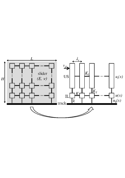
Figure 1: (color online) Sketch of the toy model. Left: A 2D rectangular slider (gray) of dimensions $L$ and $H$, of elastic constants $E$ and $\nu$, in contact with a track, is discretized into cubic blocks of size $\lambda_{c}^{3}$. Right: the slider is modeled using a 1D toy model as a bilayer. The blocks in the interfacial layer (IL) are connected through springs of stiffness $K$ (Eq. (1)). In the upper part of the slider (US), each vertical slice of material is assumed to be a rigid block connected to its neighbours through springs of stiffness $K_{L}$ (Eq. (2)). The IL and the US are connected through transverse springs of stiffness $K_{T}$ (Eq. (3)). The IL is connected with the rigid track by “frictional” springs (or $\lambda$-contacts) of elastic constant $k$. The position of the leftmost block of the US is imposed and increased at a velocity $v_{d}$.

At length scales larger than $\lambda_{c}$, the slider’s bulk is deformable and two distinct points along the interface can move by different amounts. To account for this elasticity, imagine that the slider is discretized into cubic blocks of size $\lambda_{c}^{3}$. The elastic coupling between adjacent blocks is modeled by springs connecting only the nearest neighbours, the stiffness of which can be worked out (see below) as functions of only two elastic parameters, Young’s modulus $E$ and Poisson’s ratio $\nu$. Because we aim at providing analytical solutions, we progressively reduce the dimensionality of the slider from 3D to 1D. A sketch of the final 1D model is shown in Fig. 1 (right). First the model is reduced to 2D (Fig. 1 left) by reducing the thickness of the slider to only one block’s size, $\lambda_{c}$. Then the height of the slider is modeled as a bilayer of blocks: The bottom-most layer (interfacial layer IL) is left as in the 2D model. Each block of the IL having a size $\lambda_{c}$, it is connected to the track through a single $\lambda$-contact. In the upper part of the slider (US), each vertical slice is assumed to behave rigidly, with neighbouring slices being connected by internal springs. Note that a similar, though different, model was previously introduced in BBUB2013 .

Let us consider a slider of length $L$, height $H$ and thickness $W=\lambda_{c}$ (by assumption). We assume that both $L$ and $H$ are much larger than $\lambda_{c}$. Note that in this 1D model $H$ should be interpreted as some effective height where the driving force is applied. The horizontal stiffnesses $K$ and $K_{L}$ in the IL and US, respectively, can be derived to be:

$$K=E\lambda_{c}\,$$ (1)

and

$$K_{L}\approx EH=(H/\lambda_{c})K\,.$$ (2)

The total transverse stiffness of the slider is $E/2(1+\nu)LW/H$. We assume that we can ascribe the totality of this stiffness to the $L/\lambda_{c}$ transverse springs $K_{T}$ connecting the IL to the US. $K_{T}$ thus reads:

$$K_{T}=\frac{E\lambda_{c}}{2(1+\nu)}\frac{\lambda_{c}}{H}=\frac{\lambda_{c}}{2(1+\nu)H}K.$$ (3)

Note that ${K_{T}}/{K_{L}}\sim\left({\lambda_{c}}/{H}\right)^{2}<<1$. This is a consequence of the rigid connection of the blocks constituting the US (from left to right in Fig. 1). We chose as an assumption to ascribe the totality of the transverse rigidity of the slider to only one plane between the IL and the US. Let us emphasize that, as a matter of fact, there is no exact way to capture 3D elasticity within a 1D model, even qualitatively. In particular, the stress profile in response to a side loading decays as a power law in 3D whereas it decays exponentially in 1D. The scope of our toy model is thus merely to help us investigate analytically the consequences of the self-healing nature of the rupture on the propagation length. We will see that an important parameter of the toy model is the ratio of interfacial to bulk stiffness $k/K$. The interface is denoted as stiff if $k/K\sim 1$ and soft when $k/K\ll 1$; we concentrate on the latter case which corresponds to most experimental situations.

The system can be described by three variables: $u_{t}(x)$ describes the displacement field of the US, $u(x)$ is the displacement field of the blocks in the IL, and $u_{b}(x)$ is the displacement of attachment points of the IL to the track.

The stress in the IL is then given by

$$\sigma_{c}(x)=k\,[u(x)-u_{b}(x)]/\lambda_{c}^{2}\,,$$ (4)

while the stress which is driving the IL is equal to

$$\sigma_{d}(x)=K_{T}\,[u_{t}(x)-u(x)]/\lambda_{c}^{2}\,.$$ (5)

The whole system is driven by imposing the displacement of the left-most block of the US as $u_{t}(0,t)=v_{d}t$, with $v_{d}$ an arbitrarily small velocity.

3 Self-healing slip pulse-like rupture

The frictional behaviour of each junction connecting the IL to the track is the following. It acts as a spring of elastic constant $k$ as long as its stretching remains below a critical value $u_{s}=f_{s}/k$ but breaks and immediately repins with zero stretching when the local shear stress reaches $\sigma_{s}=f_{s}/\lambda_{c}^{2}$.

When a loading is applied to the slider, it is transmitted differently to each $\lambda$-contact due to elasticity of the slider. The leftmost $\lambda$-contact is the first to reach its breaking threshold, slide and locally relax the interface. This causes an extra stress on the neighboring contacts, which tend to slide too, so that sliding events propagate as a kink, extending the initial relaxed domain. Such a scenario may be described as a solitary wave BPST2012 ; BP2012 . The rupture mode is of the self-healing slip pulse type, with a pulse width equal to the lateral size of one contact, $\lambda_{c}$, because a broken contact repins immediately, before the breaking of its neighbour. Note that, in the absence of the US, and for a displacement controlled loading of the left edge of the slider, no propagation would occur: the first block would not move after breaking of its $\lambda$-contact, and thus its right-neighbour would not be further loaded to its breaking threshold.

In order to simplify the analysis, we suppose the existence of a hierarchy of times. Namely, we assume that the pushing rate is adiabatically slow, $v_{d}\to 0$, while the sound speed (which determines the rate of propagation of the elastic stress) is very large, $v_{R}\to\infty$. Therefore, when a front propagates, it is accompanied by a quasi-static stress field defined by mechanical equilibrium of the forces acting on the interface layer (inertia effects are ignored). In the following, we show that there exist a typical length scale $\Lambda$ which characterizes the stress accumulation and thus the precursor length.

4 Equations to be solved

In the discrete model we have $x=i\lambda_{c}$, $u_{t}(x)\to u_{t,i}$, $u(x)\to u_{i}$ and $u_{b}(x)\to u_{bi}$. In equilibrium, the displacements should satisfy

$$K_{L}\,(u_{t,i+1}+u_{t,i-1}-2u_{t,i})=K_{T}\,(u_{t,i}-u_{i})\,,$$

$$K\,(u_{i+1}+u_{i-1}-2u_{i})=k\,(u_{i}-u_{bi})+K_{T}\,(u_{i}-u_{t,i})\,.$$

In the continuum approximation, these equations reduce to the set of equations:

$$u^{\prime\prime}_{t}(x)=\kappa_{T}^{2}\left[u_{t}(x)-u(x)\right],$$ (6)

$$u^{\prime\prime}(x)=\kappa^{2}\left[u(x)-w(x)\right],$$ (7)

$$w(x)=\beta\,u_{t}(x)+(1-\beta)\,u_{b}(x)\,,$$ (8)

where $\kappa_{T}=(K_{T}/K_{L})^{1/2}/\lambda_{c}$, $\kappa=[(k+K_{T})/K]^{1/2}/\lambda_{c}$ and $\beta=K_{T}/(K_{T}+k)$.

A key trick of our analytical approach is that the general solution of the equation $u^{\prime\prime}(x)=\kappa^{2}\,[u(x)-w(x)]$ is $u(x)=D\,e^{\pm\kappa x}-\kappa\int^{x}d\xi\,w(\xi)\sinh[\kappa(x-\xi)]\,$.

As we impose the position of the left-hand side (trailing edge) of the US we have

$$u_{t}(0)=U_{t}\,,$$ (9)

while the left-hand side of the IL is free so that

$$K\lambda_{c}u^{\prime}(0)+K_{T}\left[U_{t}-u(0)\right]=k\left[u(0)-u_{b}(0)\right].$$ (10)

To simplify considerations, we ignore the right-hand side boundary conditions assuming that the chain is infinite, $L\to\infty$, so that $u_{t}(\infty)=u(\infty)=u_{b}(\infty)=0$.

Let initially, at $t=0$, the system be completely relaxed: $u_{t}(x)=u(x)=0$ and $u_{b}(x)=u_{b}^{(0)}(x)=0$. We then start to push slowly the trailing edge of the US, so that $U_{t}=v_{d}t$ with $v_{d}\to 0$. The solution of Eqs. (6)–(10) is:

$$u_{t}(x)=D_{10}\,e^{-\kappa_{1}x}+D_{20}\,e^{-\kappa_{2}x},$$ (11)

$$u(x)=\alpha_{1}D_{10}\,e^{-\kappa_{1}x}+\alpha_{2}D_{20}\,e^{-\kappa_{2}x},$$ (12)

where $\kappa_{{}^{1}_{2}}^{2}=\frac{1}{2}(\kappa^{2}+\kappa_{T}^{2}\pm\sqrt{\cal D})$, $\alpha_{{}^{1}_{2}}=\frac{1}{2}[1-(\kappa^{2}\pm\sqrt{\cal D}/\kappa_{T}^{2})]$, ${\cal D}=(\kappa^{2}-\kappa_{T}^{2})^{2}+4\beta\kappa^{2}\kappa_{T}^{2}$, $D_{10}=(\alpha_{2}U_{t}-u_{c})/(\alpha_{2}-\alpha_{1})$, $D_{20}=(u_{c}-\alpha_{1}U_{t})/(\alpha_{2}-\alpha_{1})$ and $u_{c}\equiv u(0)=U_{t}\,[\lambda_{c}\beta\kappa^{2}(\kappa_{1}-\kappa_{2})+(K_{T}/K)\sqrt{\cal D}]/[\lambda_{c}\kappa_{T}^{2}(\alpha_{2}\kappa_{2}-\alpha_{1}\kappa_{1})+\lambda_{c}^{2}\kappa^{2}\sqrt{\cal D}]$.

The positions $U_{t}$ and $u_{c}$ grow together until the trailing edge of the US reaches a position $U_{t0}$ where the left end of the IL achieves the threshold value $u_{s}$ at some time $t_{1}=U_{t0}/v_{d}$. At $t=t_{1}$ the left-most $\lambda$-contact breaks and attaches again with zero stretching, $u_{b}(0)=u_{b}^{(1)}(0)=u_{s}$, and the whole system relaxes, adjusting itself to a new configuration with $u_{t}(0)=U_{t0}$, $u_{b}(0)=u_{s}$ and $u_{b}(x\geq\lambda_{c})=0$. After relaxation, all contacts have shifted to the right, so that the IL stress $\sigma_{c}(x)$ for $x\geq\lambda_{c}$ increases. As a consequence the stress on the second contact has grown above the threshold $\sigma_{s}$ so that it must break too. This domino-like process will continue until the stress at some ($s_{0}$-th) contact will remain below the threshold. This first passage distance defines a characteristic length $\Lambda=s_{0}\lambda_{c}$ which controls the kinematics of the onset of sliding.

We emphasize that the driving stress $\sigma_{d}(x)$, Eq. (5), changes self-consistently during front propagation, as $u(x)$ changes. The moving self-healing crack leaves behind itself relaxed contacts. When the front reaches a position $s$, the current shapes of the displacement fields $\widetilde{u}_{t}(x;s)$ and $\widetilde{u}(x;s)$ are given by solution of Eqs. (6)–(8). The current displacement of the bottom surface of the IL, $\widetilde{u}_{b}(x;s)$, is determined by the current propagation length of the front:

$$\widetilde{u}_{b}(x;s)=\tilde{u}(x+0;x)\;\;\;{\rm for}\;\;\;x<s,$$ (13)

while ahead the moving front the contacts are still loaded,

$$\widetilde{u}_{b}(x;s)=u_{b}^{(0)}(x)\;\;\;{\rm for}\;\;\;x>s.$$ (14)

With these conditions, the functions $\widetilde{u}_{t}(x;s)$ and $\widetilde{u}(x;s)$ take the following form. For the front tail ($x<s$):

$$\widetilde{u}_{t}(x;s)=\left[D_{11}(s)\sinh(\kappa_{1}x)+D_{12}(s)\cosh(\kappa_{1}x)\right]$$

$$\;\;\;\;\;\;\;\;\;\;\;\;+\left[D_{21}(s)\sinh(\kappa_{2}x)+D_{22}(s)\cosh(\kappa_{2}x)\right]$$

$$\;\;\;\;\;\;\;\;\;\;\;\;+\bar{u}_{t}(0;x)\,,$$ (15)

$$\widetilde{u}(x;s)=\alpha_{1}\left[D_{11}(s)\sinh(\kappa_{1}x)+D_{12}(s)\cosh(\kappa_{1}x)\right]$$

$$\;\;\;\;\;\;\;\;\;\;\,+\alpha_{2}\left[D_{21}(s)\sinh(\kappa_{2}x)+D_{22}(s)\cosh(\kappa_{2}x)\right]$$

$$\;\;\;\;\;\;\;\;\;\;\,+\bar{u}(0;x)\,,$$ (16)

where

$$\bar{u}_{t}(x_{0};x)=\int_{x_{0}}^{x}d\xi\,\widetilde{u}_{b}(\xi)\left\{b_{1}\sinh[\kappa_{1}(x-\xi)]\right.$$

$$\;\;\;\;\;\;\;\;\;\;\;\;\;\;\;\;\;\;\;\;\;\;\;\;\;\;\;\;\;\;\;\;\;\left.+\;b_{2}\sinh[\kappa_{2}(x-\xi)]\right\},$$ (17)

$$\bar{u}(x_{0};x)=\int_{x_{0}}^{x}d\xi\,\widetilde{u}_{b}(\xi)\left\{\alpha_{1}b_{1}\sinh[\kappa_{1}(x-\xi)]\right.$$

$$\;\;\;\;\;\;\;\;\;\;\;\;\;\;\;\;\;\;\;\;\;\;\;\;\;\;\;\;\;\;\;\;\left.+\;\alpha_{2}b_{2}\sinh[\kappa_{2}(x-\xi)]\right\},$$ (18)

with $b_{1}=(1-\beta)\kappa^{2}/\kappa_{1}(\alpha_{2}-\alpha_{1})$ and $b_{2}=-b_{1}\kappa_{1}/\kappa_{2}$. Ahead of the front ($x>s$):

$$\widetilde{u}_{t}(x;s)=D_{1}(s)\,e^{-\kappa_{1}(x-s)}+D_{2}(s)\,e^{-\kappa_{2}(x-s)}$$

$$\;\;\;\;\;\;\;\;\;\;\;\;\;\;\;\;\;\;\;\;\;\;\;\;\;\;\;\;\;\;\;\;\;+\bar{u}_{t}(s;x)\,,$$ (19)

$$\widetilde{u}(x;s))=\alpha_{1}D_{1}(s)\,e^{-\kappa_{1}(x-s)}+\alpha_{2}D_{2}(s)\,e^{-\kappa_{2}(x-s)}$$

$$\;\;\;\;\;\;\;\;\;\;\;\;\;\;\;\;\;\;\;\;\;\;\;\;\;\;\;\;\;\;\;\;\;+\bar{u}(s;x)\,.$$ (20)

The coefficients $D_{1}(s)$, $D_{2}(s)$, $D_{11}(s)$, $D_{12}(s)$, $D_{21}(s)$ and $D_{22}(s)$ in Eqs. (15)–(20) are functionals of the function $u_{b}^{(0)}(x)$ and should be determined by the two left-hand-side boundary conditions (9) and (10) and the following four continuity conditions at $x=s\pm 0$:

$$\widetilde{u}_{t}(s-0;s)=\widetilde{u}_{t}(s+0;s)\,,$$ (21)

$$\widetilde{u}_{t}^{\prime}(s-0;s)=\widetilde{u}_{t}^{\prime}(s+0;s)\,,$$ (22)

$$\widetilde{u}(s-0;s)=\widetilde{u}(s+0;s)\,,$$ (23)

$$\widetilde{u}^{\prime}(s-0;s)=\widetilde{u}^{\prime}(s+0;s)\,,$$ (24)

which finally lead to a set of integral equations that has to be solved self-consistently.

5 Numerical solution

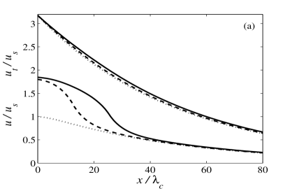
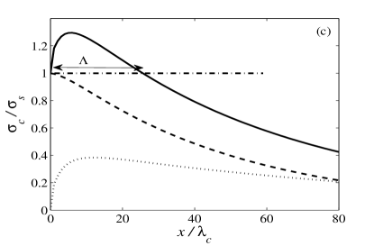
Figure 2: (a) Displacement fields $\widetilde{u}_{t}(x;s)$ and $\widetilde{u}(x;s)$: when the front nucleates at $t=t_{1}$ ($s=0$, dotted, $u_{t}(x,0)\approx U_{t0}e^{-\kappa_{2}x}$) and during front propagation for the distances $s=13\,a$ (dashed) and $s=26\,a$ (full precursor propagation length, solid curve). (b) Stress field in the IL during front propagation. (c) Dashed line: shear stress in the IL at front nucleation ($t=t_{1}-0$). Solid line: shear stress in the IL, at the front tip, when it passes at location $x$ ($s=x$) during its propagation. Dotted line: extra stress $\Delta\sigma_{c}(s)$. $H/\lambda_{c}=25$, $k/K=0.03$, $\nu=0.3$, $L=100\lambda_{c}$.

A typical solution of the equations for the first front passage, for a completely relaxed IL initially ($u_{b}^{(0)}(x)=0$), is shown in Fig. 2. We have assumed that front propagation is fast compared with the slow pushing, so that the left-most block of the US has no opportunity to move before the precursor arrests.

In these conditions, and when the slider’s height is much larger than $\lambda_{c}$, the displacement field in the US is approximately unchanged upon propagation of the precursor, even if the displacement in the IL almost double upon front propagation (Fig. 2(a)). Because the $\lambda$-contacts repin immediately after breaking, they also immediately start to load again as the next $\lambda$-contacts relax and the precursor propagates. As a consequence, the stress behind the front is increasing with the distance to the front (Fig. 2(b)). Ahead of the front, the relaxed $\lambda$-contacts induce an extra loading of the unbroken contacts ahead of the front, characterized by a stress peak at the front location (Fig. 2(b)). This extra stress $\Delta\sigma_{c}$ is enough to bring initially less stressed contacts up to their threshold. However, because the initial stress is a decaying function of $x$, the extra stress is sufficient to bring the contacts above their threshold only over a finite length $\Lambda$ (Fig. 2(c)).

6 Analytical solution

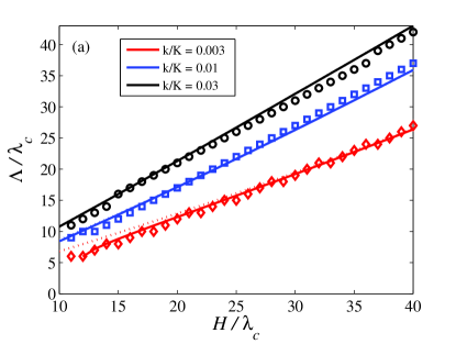
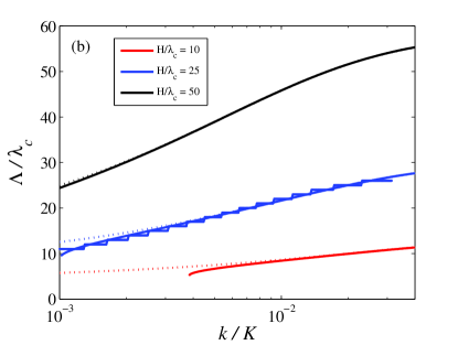
Figure 3: (color online) Dependence of the characteristic length $\Lambda$ on model parameters. Symbols are for numerics, solid lines for analytics, dotted lines for approximate analytics (Eq. 66). (a) $\Lambda$ versus $H/\lambda_{c}$ for different values of the interface stiffness $k/K=0.03$ (diamonds, red), 0.01 (squares, blue) and 0.003 (circles, black). (b) $\Lambda$ versus $k/K$ for fixed $H/\lambda_{c}$=10 (bottom, red), 25 (middle, blue, dots), 50 (top, black). $\nu=0.3$, $L/\lambda_{c}=100$.

For the first precursor arising from a completely relaxed IL ($u_{b}^{(0)}(x)=0$), we found some analytical results. The full proof is available in Appendix. Here, we will only provide the main results and the assumptions made to get them.

We assume that the elastic correlation length is much smaller than the slider’s thickness ($\lambda_{c}\ll H$). Since $\lambda_{c}$ is typically in the micrometer range, this assumption is valid for a large range of macroscopic systems. We also assume that the interfacial stiffness is much smaller than the internal stiffness of the slider ($k\ll K$). For rough interfaces, this assumption is also generally true PSD2013 . Based on the results of Fig. 2(a), we assume that the displacement field in the US is given by $u_{t}(x)\approx U_{t0}e^{-\kappa_{2}x}$ and does not change during front propagation. Under these assumptions, we find an analytical expression for the length $\Lambda$ of the first precursor (Eq. (66) in the Appendix). This expression approximates, for $\Lambda\gg\kappa^{-1}$ (i.e. large $H/\lambda_{c}$ and/or $k/K$), to

$$\Lambda\approx\kappa_{2}^{-1}\ln\left\{2/[(1+\beta-2\kappa_{2}/\kappa)\,\Psi_{1}]\right\},$$ (25)

where $\Psi_{1}=1+\lambda_{c}\kappa_{2}/(1+\lambda_{c}\kappa)$.

The analytical results are shown in Fig. 3. $\Lambda$ is found to increase quasi-linearly with the height of the slider (Fig. 3(a)) and to increase quasi-logarithmically with the stiffness of the interface (Fig. 3(b)). Comparison with the numerical results shows a quantitative agreement. We also checked that molecular dynamics simulations of the model agree with the analytical results (not shown).

7 Discussion

As for any toy model, we cannot expect our model to reproduce quantitatively experimental results. In this discussion, we will thus mainly list the consequences of the various simplifying assumptions that we made in order to allow for an analytical solution.

We have shown that in our model, the onset of sliding is characterized by precursory self-healing slip pulses. The characteristic length $\Lambda$ of the first precursor is controlled by two parameters, $H/\lambda_{c}$ and $k/K$, determined by the slider and interface properties. Importantly, $\Lambda$ does not depend on the threshold value $\sigma_{s}$. This result is due to the fact that we use linear elasticity and immediate repinning of $\lambda$-contacts in a completely relaxed state. As a consequence, all curves Fig.2(c) are unmodified if $\sigma_{s}$ is changed, and thus the length $\Lambda$ is also unchanged.

This threshold-independence of $\Lambda$ would mean that, if the interface would obey Amontons’ law of friction ($\sigma_{s}=\mu_{s}\sigma_{n}$, with $\mu_{s}$ the static friction coefficient and $\sigma_{n}$ the normal stress) locally (at the $\lambda$-contacts scale), $\Lambda$ would not depend on $\mu_{s}$. This is a major difference with previous precursor models SD2010 ; TSATM2011 ; ASTTM2012 , in which the length of the first (crack-like) precursor depends explicitly on $\mu_{s}$. The independence of $\Lambda$ with $\mu_{s}$ implies an independence with the normal load on the system, as long as the type of loading (pure side loading) is unchanged.

If an additional uniform shear stress $\sigma_{0}$ is applied to the top surface of the slider, then the threshold will decrease, $\sigma_{s}\to\sigma_{s}-\sigma_{0}$. In such conditions, the crack will nucleate at a lower macroscopic force and will propagate over a longer distance. Moreover, if $\sigma_{0}>\sigma_{f}$, where $\sigma_{f}$ is the Griffith threshold (see e.g. Eq. (35) in Ref.[14] obtained for a simpler 1D model), then the crack will never stop, so that $\Lambda\to\infty$.

We have considered a constant value of $\sigma_{s}$ along the interface. Let us consider a non-uniform normal load of the form $\sigma_{n}(x)=\sigma_{n0}+\epsilon x$, as in top-driven systems with friction-induced torque SD2010 . The thresholds thus also depend on $x$, $\sigma_{s}(x)=\sigma_{s0}+\mu_{s}\epsilon x$. $\Lambda$ will depend on the asymmetry parameter $\epsilon$ roughly as $\Lambda(\epsilon)\approx\Lambda(0)(1-\epsilon)$.

We have assumed that broken contacts are immediately restored with zero stretching. Instead, one may assume that the contacts repin after some delay time $\tau_{d}$ BBU2009 ; BPST2012 ; BP2012 ; TTSMS2014 ; TSSTAM2014 . Assuming a constant $\tau_{d}$, the width of the self-healing crack will increase from $\lambda_{c}$ to $v\tau_{d}$, with $v$ the (minimal) propagation velocity of the front (see Refs. BPST2012 ; BP2012 ), and the length $\Lambda$ will increase to $\Lambda+v\tau_{d}$. Note that experimentally, the repinning conditions is generally unraveled. In gels however, the interface was reported to re-stick when the slip velocity behind the rupture tip decreases back to a critical velocity depending of the gel composition BCR2003 ; RBH2011 .

In the presence of inertia, which has been neglected in the present quasi-static model, the IL blocks will be able to continue increasing the load on their right-hand neighbours even after repinning of their individual $\lambda$-contacts. This extra loading is expected to help breaking further contacts and thus increase the precursor length. In contrast, the front nucleation process will be unaffected because it originates from a static state of the system.

We have assumed that all $\lambda$-contacts behave as classical springs with a sawtooth-shape dependence $u(\sigma_{c}$). In real systems, they are composed of $N_{c}$ micro-junctions with a distribution of thresholds $P_{c}(f_{s})$. If $P_{c}(f_{s})$ is wide enough, the elastic instability will disappear, and the $\lambda$-contacts will smoothly slide with the pushing velocity $v_{d}$ after reaching the stretching $u_{s}$ BP2008 ; BP2010 . No discrete precursor will thus be observed, as a quasi-static front will continuously run through the interface.

Here we have considered the first precursor only. After its propagation, the system is left in the stress state shown in solid line in Fig. 2(b). If the system is further loaded, the left-most $\lambda$-contact will again be the first to reach its breaking threshold, and a second precursor will nucleate. It will propagate through the stress field left by the previous event, itself modified by the additional loading and this scenario will repeat itself. We have run numerical simulations for the series of precursors and found that all precursors propagate roughly over the same length $\Lambda$ (between precursors, the stress peak left at the precursor extremity does propagate further quasi-statically due to the increased external loading). This is not in agreement with experimental data RCF2007 ; MSN2010 and previous precursor models producing crack-like (rather than self-healing-like) rupture MSN2010 ; SD2010 ; TSATM2011 ; ASTTM2012 , in which successive precursors propagate over increasing lengths.

This discrepancy disappears if aging of the $\lambda$-contacts — a newborn contact has a smaller size and thus a lower breaking threshold force $f_{s}$ — is taken into account BP2010 ; BP2013 . We checked this numerically by considering a time-increasing $f_{s}$. The previously broken region of the interface is characterized by “younger” contacts and therefore by smaller thresholds than the “old” unbroken part of the system. Hence, the next front will pass this region more easily and propagate deeper into the system. This process repeats itself until a precursor would span the whole interface and trigger macroscopic sliding of the interface. Note that in these numerical results, there is a competition between the aging and loading time scales, while the front propagation time scale is kept much smaller than the loading time scale.

The proposed toy model is important for all systems in which friction instabilities are central, from tribology to geophysics. It helps clarifying the problem of the selection of the size of the part of the interface which will slip as a function of the bulk material properties, interfacial parameters and loading conditions. It will be particularly relevant to systems in which self-healing slip-pulses have been observed (e.g. LRR2006 ; RBH2011 ; RWDP2014 ). Our results emphasize the fact that the behaviour of precursors is intimately related to the repinning rule of the interface (at vanishing velocity for crack-like rupture; immediately in the present model). We thus advocate for an increased experimental effort to better constrain these repinning rules, which will be very useful to propose improved models for the onset of frictional sliding.

Appendix: Analytical derivation of Eq. (25) in the main text

Let us introduce two dimensionless parameters

$$h\equiv\lambda_{c}/H\;\;\;{\rm and}\;\;\;q\equiv k/K\,,$$ (26)

so that $K_{L}=K/h$, $K_{T}=Kh/2(1+\sigma)$, $\beta=1/(1+b)$, $1-\beta=b/(1+b)$, $(\lambda_{c}\kappa_{T})^{2}=hq/b$, $(\lambda_{c}\kappa)^{2}=q\,(1+b)/b$,

$$\varepsilon\equiv\frac{\kappa_{T}^{2}}{\kappa^{2}}=\frac{h}{1+b}\,,$$ (27)

where $b=2(1+\sigma)q/h$, and consider the typical system with $h,q\ll 1$. In this case $\varepsilon\ll 1$, so that $\kappa_{1}^{2}\approx\kappa^{2}(1+\beta\varepsilon)$ and $\kappa_{2}^{2}\approx\kappa^{2}\varepsilon\,(1-\beta)=q\varepsilon/\lambda_{c}^{2}$, or

$$(\lambda_{c}\kappa_{2})^{-1}\approx[2(1+\sigma)+h/q]^{1/2}/h\,.$$ (28)

In accordance with the numerics (see Fig. 2(a)), let us assume that in the case of $h,q\ll 1$ the displacement field in the US is given by

$$u_{t}(x)\approx U_{t0}e^{-\kappa_{2}x}$$ (29)

and does not change during front propagation. Before nucleation of the first precursor, the solution of Eq. (7) in the main text is

$$u(x)=A_{30}\sinh(\kappa x)+A_{40}\cosh(\kappa x)$$

$$-\kappa\beta U\int_{0}^{x}d\xi\,e^{-\kappa_{2}\xi}\sinh[\kappa(x-\xi)]$$

$$=\frac{1}{2}\left(A_{40}+A_{30}-\frac{1}{2}\,\beta U\frac{\kappa}{\kappa+\kappa_{2}}\right)e^{\kappa x}$$

$$+\frac{1}{2}\left(A_{40}-A_{30}-\beta U\frac{\kappa}{\kappa-\kappa_{2}}\right)e^{-\kappa x}$$

$$+\beta U\frac{\kappa^{2}}{\kappa^{2}-\kappa_{2}^{2}}e^{-\kappa_{2}x}.$$ (30)

The right-hand-side boundary condition, $u(x)\to 0$ at $x\to\infty$, gives us

$$A_{40}+A_{30}=\frac{1}{2}\,\beta U\frac{\kappa}{\kappa+\kappa_{2}}\;,$$ (31)

while the left-hand-side boundary condition (Eq. (10) in the main text) leads to the equation

$$(A_{40}-A_{30})(1+\lambda_{c}\kappa)(\kappa+\kappa_{2})=\beta U\kappa(1+a\kappa+2\lambda_{c}\kappa_{2})\,.$$ (32)

Thus, before nucleation of the first precursor, the IL displacement field is

$$u(x)=\frac{\beta U\kappa^{2}}{(\kappa^{2}-\kappa_{2}^{2})}\left(e^{-\kappa_{2}x}-\frac{\kappa_{2}}{\kappa}\frac{(1+\lambda_{c}\kappa_{2})}{(1+\lambda_{c}\kappa)}\,e^{-\kappa x}\right).$$ (33)

Equation (33) allows us to couple the parameters $U\equiv u_{t}(0)$ and $u_{c}\equiv u(0)$:

$$U=u_{c}\left(1+\frac{\kappa_{2}}{\kappa}\right)/(\beta\Psi_{1})\,,$$ (34)

where

$$\Psi_{1}=1+\frac{\kappa_{2}}{\kappa}\frac{\lambda_{c}\kappa}{(1+\lambda_{c}\kappa)}\,.$$ (35)

When the displacement of the IL trailing edge reaches the threshold value $u_{s}$ at some $U=U_{0}=u_{s}(1+\kappa_{2}/\kappa)/(\beta\Psi_{1})$, the front starts to propagate. In this case the solution of Eq. (7) in the main text, ahead of the propagating front, $x>s$, where $u_{b}(x)=0$ so that $w(x)=\beta u_{t}(x)=\beta U_{0}e^{-\kappa_{2}x}$, is given by

$$\widetilde{u}(x;s)=A_{3}(s)\,e^{-\kappa(x-s)}+A_{4}(s)\,e^{\kappa(x-s)}$$

$$-\kappa\beta U_{0}\int_{s}^{x}d\xi\,e^{-\kappa_{2}\xi}\sinh[\kappa(x-\xi)]$$

$$=\frac{\beta U_{0}\kappa^{2}e^{-\kappa_{2}x}}{(\kappa^{2}-\kappa_{2}^{2})}+A_{3}(s)\,e^{-\kappa(x-s)}+A_{4}(s)\,e^{\kappa(x-s)}$$

$$-\frac{1}{2}\,\beta U_{0}\kappa\,e^{-\kappa_{2}s}\left[\frac{e^{\kappa(x-s)}}{(\kappa+\kappa_{2})}+\frac{e^{-\kappa(x-s)}}{(\kappa-\kappa_{2})}\right]\,.$$ (36)

The right-hand-side boundary condition gives us the coefficient $A_{4}(s)$,

$$A_{4}(s)=\frac{1}{2}\,\beta U_{0}\frac{\kappa\,e^{-\kappa_{2}s}}{(\kappa+\kappa_{2})}\,,$$ (37)

so that Eq. (36) takes the form

$$\widetilde{u}(x;s)=\frac{\beta U_{0}\kappa^{2}}{(\kappa^{2}-\kappa_{2}^{2})}\;e^{-\kappa_{2}x}$$

$$+\left[A_{3}(s)-\frac{1}{2}\,\beta U_{0}\frac{\kappa\,e^{-\kappa_{2}s}}{(\kappa-\kappa_{2})}\right]e^{-\kappa(x-s)}.$$ (38)

Behind the propagating front, $x<s$, where $w(x)=\beta\,u_{t}(x)+(1-\beta)\,u_{b}(x)$ and $u_{b}(x)=\widetilde{u}(x+0;x)=A_{3}(x)+A_{4}(x)$, the solution of Eq. (7) in the main text is given by

$$\widetilde{u}(x;s)=A_{1}(s)\sinh(\kappa x)+A_{2}(s)\cosh(\kappa x)$$

$$-\kappa\,(1-\beta)\int_{0}^{x}d\xi\,[A_{3}(\xi)+A_{4}(\xi)]\,\sinh[\kappa(x-\xi)]$$

$$-\kappa\beta U_{0}\int_{0}^{x}d\xi\,e^{-\kappa_{2}\xi}\sinh[\kappa(x-\xi)]$$

$$=\beta U_{0}{\cal F}(x)+A_{1}(s)\sinh(\kappa x)+A_{2}(s)\cosh(\kappa x)$$

$$-\kappa\,(1-\beta)\int_{0}^{x}d\xi\,A_{3}(\xi)\,\sinh[\kappa(x-\xi)]\,,$$ (39)

where

$${\cal F}(x)=\frac{\Psi_{2}\kappa^{2}}{(\kappa^{2}-\kappa_{2}^{2})}$$

$$\times\left(\frac{\kappa_{2}}{\kappa}\sinh(\kappa x)-\cosh(\kappa x)+e^{-\kappa_{2}x}\right),$$ (40)

$$\frac{{\cal F}^{\prime}(x)}{\kappa}=\frac{\Psi_{2}\kappa^{2}}{(\kappa^{2}-\kappa_{2}^{2})}$$

$$\times\left(\frac{\kappa_{2}}{\kappa}\cosh(\kappa x)-\sinh(\kappa x)-\frac{\kappa_{2}}{\kappa}\,e^{-\kappa_{2}x}\right),$$ (41)

$$\Psi_{2}=\frac{(3-\beta)\kappa+2\kappa_{2}}{2(\kappa+\kappa_{2})}\,,$$ (42)

so that ${\cal F}(0)=0$ and ${\cal F}^{\prime}(0)=0$.

The coefficients $A_{\dots}(s)$ in these equations are determined by the boundary and continuity conditions. The left-hand-side boundary condition (Eq. (10) in the main text) couples the coefficients $A_{1}(s)$ and $A_{2}(s)$. Using $u_{b}(0)=u_{s}$, $\widetilde{u}(0;s)=A_{2}(s)$ and $\widetilde{u}^{\prime}(0;s)=\kappa A_{1}(s)$, we obtain

$$A_{2}(s)-(\lambda_{c}\kappa)^{-1}A_{1}(s)=\Psi_{3}\,,$$

$$\Psi_{3}=\beta U_{0}+(1-\beta)\,u_{s}\,.$$ (43)

The continuity conditions (Eqs. (23) and (24) in the main text) lead to two equations

$$\kappa \,(1-\beta)\int_{0}^{s}d\xi\,A_{3}(\xi)\,\sinh[\kappa(s-\xi)]+A_{3}(s)$$

$$=A_{1}(s)\sinh(\kappa s)+A_{2}(s)\cosh(\kappa s)+\beta U_{0}\Psi_{4}(s)$$ (44)

and

$$\kappa \,(1-\beta)\int_{0}^{s}d\xi\,A_{3}(\xi)\,\cosh[\kappa(s-\xi)]-A_{3}(s)$$

$$=A_{1}(s)\cosh(\kappa s)+A_{2}(s)\sinh(\kappa s)+\beta U_{0}\Psi_{5}(s)\,,$$ (45)

where

$$\Psi_{4}(s)={\cal F}(s)-\frac{\kappa\,e^{-\kappa_{2}s}}{2(\kappa+\kappa_{2})}\;,$$ (46)

$$\Psi_{5}(s)=\frac{{\cal F}^{\prime}(s)}{\kappa}-\frac{\kappa\,e^{-\kappa_{2}s}}{2(\kappa+\kappa_{2})}\;.$$ (47)

Taking the difference and sum of Eqs. (44) and (45), we obtain two new equations:

$$2A_{3}(s)\,e^{\kappa s}-\kappa\,(1-\beta)\int_{0}^{s}d\xi\,A_{3}(\xi)\,e^{\kappa\xi}$$

$$=A_{2}(s)-A_{1}(s)+\beta U_{0}[\Psi_{4}(s)-\Psi_{5}(s)]\,e^{\kappa s},$$ (48)

$$\kappa\,(1-\beta)\int_{0}^{s}d\xi\,A_{3}(\xi)\,e^{-\kappa\xi}$$

$$=A_{2}(s)+A_{1}(s)+\beta U_{0}\left[\Psi_{4}(s)+\Psi_{5}(s)\right]\,e^{-\kappa s}.$$ (49)

Using Eq. (43), Eqs. (46) and (47) may be rewritten as

$$2A_{3}(s)\,e^{\kappa s} -\kappa\,(1-\beta)\int_{0}^{s}d\xi\,A_{3}(\xi)\,e^{\kappa\xi}=A_{1}(s)\frac{(1-\lambda_{c}\kappa)}{\lambda_{c}\kappa}$$

$$+\Psi_{3}+\beta U_{0}[\Psi_{4}(s)-\Psi_{5}(s)]\,e^{\kappa s},$$ (50)

$$\kappa\,(1 -\beta)\int_{0}^{s}d\xi\,A_{3}(\xi)\,e^{-\kappa\xi}=A_{1}(s)\frac{(1+\lambda_{c}\kappa)}{\lambda_{c}\kappa}$$

$$+\Psi_{3}+\beta U_{0}\left[\Psi_{4}(s)+\Psi_{5}(s)\right]\,e^{-\kappa s}.$$ (51)

Combining these equations, we finally come to the integral equation for the coefficient $A_{3}(s)$:

$$A_{3}(s)(1+\lambda_{c}\kappa)\,e^{\kappa s}$$

$$-\kappa(1-\beta)\int_{0}^{s}d\xi\,A_{3}(\xi)\,[\cosh(\kappa\xi)+(\lambda_{c}\kappa)\sinh(\kappa\xi)]$$

$$=\lambda_{c}\kappa\Psi_{3}+\beta U_{0}\Psi_{2}\Psi_{6}(s)\,,$$ (52)

where

$$\Psi_{6}(s) =\frac{\kappa\,(1+\lambda_{c}\kappa)}{2(\kappa-\kappa_{2})}\,e^{(\kappa-\kappa_{2})s}$$

$$-\frac{\kappa\,(\lambda_{c}\kappa^{2}+\kappa_{2})}{(\kappa^{2}-\kappa_{2}^{2})}\left[1+e^{-(\kappa+\kappa_{2})s}\right]$$ (53)

so that

$$\Psi_{6}^{\prime}(s)=\left[\frac{(1+\lambda_{c}\kappa)}{2}\,e^{\kappa s}+\frac{(\lambda_{c}\kappa^{2}+\kappa_{2})}{(\kappa-\kappa_{2})}\,e^{-\kappa s}\right]\kappa\,e^{-\kappa_{2}s}.$$ (54)

From Eq. (52) we find that

$$A_{3}(0)=[\lambda_{c}\kappa\Psi_{3}+\beta U_{0}\Psi_{2}\Psi_{6}(0)]/(1+\lambda_{c}\kappa)\,.$$ (55)

Differentiating Eq. (52), we obtain a differential equation for $A_{3}(s)$:

$$\frac{1}{\kappa}\,A^{\prime}_{3}(s)+A_{3}(s)=A_{3}(s)\,\frac{(1-\beta)}{(1+\lambda_{c}\kappa)}$$

$$\times[\cosh(\kappa s)+(\lambda_{c}\kappa)\sinh(\kappa s)]\,e^{-\kappa s}$$

$$+\frac{\beta U_{0}\Psi_{2}}{\kappa\,(1+\lambda_{c}\kappa)}\Psi_{6}^{\prime}(s)\,e^{-\kappa s}$$ . (56)

From Eq. (56) we obtain that at short distances, $s\ll\kappa^{-1}$, $A_{3}(s)\approx A_{3}(0)(1+\gamma_{3}s)$, where

$$\gamma_{3}=-\frac{\kappa}{1+\lambda_{c}\kappa}\left[\beta+\lambda_{c}\kappa-\frac{\beta U_{0}}{A_{3}(0)}\Psi_{2}\frac{\Psi_{6}^{\prime}(0)}{\kappa}\right].$$ (57)

From Eqs. (37) and (56) it follows that $\widetilde{u}(s+0;s)=A_{3}(s)+A_{4}(s)\approx A_{0}\,(1+\gamma s)$ at short distances, $s\ll\kappa^{-1}$, where

$$A_{0}=A_{3}(0)+A_{4}(0)$$ (58)

and

$$\gamma=[\gamma_{3}A_{3}(0)-\kappa_{2}A_{4}(0)]/A_{0}\,,$$ (59)

while for long distances, $s\gg\kappa^{-1}$, $\widetilde{u}(s+0;s)$ decays exponentially,

$$\widetilde{u}(s+0;s)\approx{\cal A}\,e^{-\kappa_{2}s},$$

$${\cal A}=\beta U_{0}\left[\frac{\kappa}{2(\kappa+\kappa_{2})}+\frac{\Psi_{2}}{(1+\beta-2\kappa_{2}/\kappa)}\right].$$ (60)

The function $\widetilde{u}(s+0;s)$ may be approximated as

$$\widetilde{u}(s+0;s)\approx A_{0}\;\frac{(1+C)^{\alpha}\,e^{\kappa_{3}s}}{(e^{\kappa_{3}s}+C)^{\alpha}}\;,$$ (61)

where

$$\alpha=1+\kappa_{2}/\kappa_{3}\,,$$ (62)

$$C=(\kappa_{2}+\gamma)/(\kappa_{3}-\gamma)\,,$$ (63)

and comparing Eqs. (59) and (61), we obtain a nonlinear equation, which defines the value $\kappa_{3}$:

$$\ln\frac{\cal A}{A_{0}}=\left(1+\frac{\kappa_{2}}{\kappa_{3}}\right)\ln\frac{\kappa_{2}+\kappa_{3}}{\kappa_{3}-\gamma}\,.$$ (64)

Then, the IL stress ahead of the front is $\sigma_{c}(s)=k\,\widetilde{u}(s+0;s)/\lambda_{c}^{2}$, and the equation $\sigma_{c}(\Lambda)=\sigma_{s}$ defines the characteristic length $\Lambda$:

$$\Lambda\approx\kappa_{3}^{-1}\ln y\,,$$ (65)

where $y$ is determined by the solution of the equation ${\cal B}y=(y+C)^{\alpha}$ with ${\cal B}=(1+C)^{\alpha}kA_{0}/(\sigma_{s}\lambda_{c}^{2})$.

Using Eq. (60), $\Lambda$ may approximately be presented as

$$\Lambda \approx\kappa_{2}^{-1}\ln\left(k{\cal A}/\sigma_{s}\lambda_{c}^{2}\right)$$

$$=\frac{1}{\kappa_{2}}\ln\left[\frac{2}{(1+\beta-2\kappa_{2}/\kappa)\,\Psi_{1}}\right].$$ (66)

Equation (65) corresponds to the analytical solution for $\Lambda$, whereas Eq. (66) corresponds to the approximated analytical solution provided as Eq. (25) in the main text.

References

- (1) Persson B.N.J.: Sliding Friction: Physical Principles and Applications. Springer-Verlag, Berlin (1998)
- (2) Braun O.M., Naumovets A.G.: Nanotribology: Microscopic mechanisms of friction, Surf. Sci. Rep. 60, 79 (2006)
- (3) Chateauminois A., Fretigny C., Olanier L.: Friction and shear fracture of an adhesive contact under torsion, Phys. Rev. E 81, 026106 (2010)
- (4) Prevost A., Scheibert J., Debrégeas G.: Probing the micromechanics of a multi-contact interface at the onset of frictional sliding, Eur. Phys. J. E 36, 17 (2013)
- (5) Rubinstein S.M., Cohen G., Fineberg J.: Detachment fronts and the onset of dynamic friction, Nature 430, 1005 (2004)
- (6) Rubinstein S.M., Cohen G., Fineberg J.: Dynamics of precursors to frictional sliding, Phys. Rev. Lett. 98, 226103 (2007)
- (7) Maegawa S., Suzuki A., Nakano K.: Precursors of Global Slip in a Longitudinal Line Contact Under Non-Uniform Normal Loading, Tribol. Lett. 38, 313 (2010)
- (8) Romero V.,Wandersman E., Debrégeas G., Prevost A.: Probing Locally the Onset of Slippage at a Model Multicontact Interface, Phys. Rev. Lett. 112, 094301 (2014)
- (9) Trømborg J.K, Sveinsson H.A., Scheibert J., Thøgersen K., Amundsen D.S., Malthe-Sørenssen A.: Slow slip and the transition from fast to slow fronts in the rupture of frictional interfaces, P. Natl. Acad. Sci. USA 111, 8764-8769 (2014)
- (10) Braun O.M., Barel I., Urbakh M.: Dynamics of Transition from Static to Kinetic Friction, Phys. Rev. Lett. 103, 194301 (2009)
- (11) Scheibert J., Dysthe D.K.: Role of friction-induced torque in stick-slip motion, EPL 92, 54001 (2010)
- (12) Amundsen D.S., Scheibert J., Thøgersen K., Trømborg J., Malthe-Sørenssen A.: 1D Model of Precursors to Frictional Stick-Slip Motion Allowing for Robust Comparison with Experiments, Tribol. Lett. 45, 357 (2012)
- (13) Trømborg J., Scheibert J., Amundsen D.S., Thøgersen K., Malthe-Sørenssen A.: Transition from Static to Kinetic Friction: Insights from a 2D Model, Phys. Rev. Lett. 107, 074301 (2011)
- (14) Braun O.M., Peyrard M., Stryzheus D.V., Tosatti E.: Collective Effects at Frictional Interfaces, Tribol. Lett. 48, 11 (2012)
- (15) Braun O.M., Peyrard M.: Crack in the frictional interface as a solitary wave, Phys. Rev. E 85, 026111 (2012)
- (16) Lykotrafitis G., Rosakis A.J., Ravichandran G.: Self-healing pulse-like shear ruptures in the laboratory, Science 313, 1765 (2006)
- (17) Ronsin O., Baumberger T., Hui C.Y.: Nucleation and Propagation of Quasi-Static Interfacial Slip Pulses, J. Adhesion 87, 504 (2011)
- (18) Baumberger T., Caroli C., Ronsin O.: Self-healing slip pulses and the friction of gelatin gels, Eur. Phys. J. E 11, 85 (2003)
- (19) Brörmann K., Barel I., Urbakh M., Bennewitz R.: Friction on a Microstructured Elastomer Surface, Tribol. Lett. 50, 3 (2013)
- (20) Caroli C., Nozieres P.: Hysteresis and elastic interactions of microasperities in dry friction, Eur. Phys. J. B 4, 233 (1998)
- (21) Thøgersen K., Trømborg J.K., Sveinsson H.A., Malthe-Sørenssen A., Scheibert J.: History-dependent friction and slow slip from time-dependent microscopic junction laws studied in a statistical framework, Phys. Rev. E 89, 052401 (2014)
- (22) Braun O.M., Peyrard M.: Modeling friction on a mesoscale: Master equation for the earthquakelike model, Phys. Rev. Lett. 100, 125501 (2008)
- (23) Braun O.M., Peyrard M.: Master equation approach to friction at the mesoscale, Phys. Rev. E 82, 036117 (2010)
- (24) Braun O.M., Peyrard M.: Role of aging in a minimal model of earthquakes, Phys. Rev. E 87, 032808 (2013)