Second-order interaction corrections to the Fermi surface and the quasiparticle properties of dipolar fermions in three dimensions

Abstract

We calculate the renormalized Fermi surface and the quasiparticle properties in the Fermi liquid phase of three-dimensional dipolar fermions to second order in the dipole-dipole interaction. Using parameters relevant to an ultracold gas of erbium atoms, we find that the second-order corrections typically renormalize the Hartree-Fock results by less than one percent. On the other hand, if we use the second-order correction to the compressibility to estimate the regime of stability of the system, the point of instability is already reached for a significantly smaller interaction strength than in the Hartree-Fock approximation.

I Introduction

During the last decade, the field of ultracold fermionic gases with large dipole-dipole interaction has seen rapid advances. Atomic dipolar gases have been created using ^53Cr Chicireanu et al. (2006), ^161Dy Lu et al. (2012); Burdick et al. (2015), and ^167Er Aikawa et al. (2014a, b), while molecular dipolar gases have been realized with RbCs Sage et al. (2005), LiCs Deiglmayr et al. (2008, 2010); Repp et al. (2013), NaLi Heo et al. (2012), NaK Wu et al. (2012), and KRb Ospelkaus et al. (2008); Ni et al. (2008); Ospelkaus et al. (2009); Ni et al. (2010); de Miranda et al. (2011). This has caused a surge of theoretical interest in these systems Baranov (2008); Baranov et al. (2012); Chan et al. (2010); Yamaguchi et al. (2010); Lu et al. (2013); Góral et al. (2001); Miyakawa et al. (2008); Fregoso et al. (2009); Fregoso and Fradkin (2010); Ronen and Bohn (2010); Baillie and Blakie (2010). Calculations in two Chan et al. (2010); Yamaguchi et al. (2010); Lu et al. (2013) and three Góral et al. (2001); Miyakawa et al. (2008); Fregoso et al. (2009); Fregoso and Fradkin (2010); Chan et al. (2010); Ronen and Bohn (2010); Baillie and Blakie (2010) dimensions have led to the prediction that in the regime where the Fermi liquid phase is stable, the anisotropy of the dipolar interaction leads to a nematic deformation of the Fermi surface as well as to anisotropic quasiparticle properties. Very recently this prediction has partly been confirmed experimentally for a three-dimensional system by Aikawa et al. Aikawa et al. (2014b), who cooled fermionic ${}^{167}\text{Er}$ atoms, confined in a three-dimensional harmonic trap, well below the Fermi temperature $T_{F}$ and probed them via time-of-flight measurements. They found that the Fermi surface indeed elongates along the direction of the external field, in good agreement with theoretical predictions.

Due to the partly attractive nature of the dipole-dipole interaction, it is expected that for a strong enough interaction (or high enough density) the normal Fermi liquid phase becomes unstable, giving rise to superfluid Baranov et al. (2002); Bruun and Taylor (2008); Cooper and Shlyapnikov (2009); Zhao et al. (2010); Liao and Brand (2010), liquid crystalline Fregoso et al. (2009); Fregoso and Fradkin (2009); Quintanilla et al. (2009); Carr et al. (2009); Maeda et al. (2013), density wave Sun et al. (2010); Mikelsons and Freericks (2011); Parish and Marchetti (2012); Block and Bruun (2014), or Wigner crystal phases Matveeva and Giorgini (2012); Babadi et al. (2013). In contrast, for a rapidly rotating 2D system of dipolar fermions the Wigner crystal phase is possibly the ground state for low densities, while for higher densities it turns into a Laughlin liquid state Baranov et al. (2005, 2008). Further studies focused on finite-temperature effects Zhang and Yi (2010); Endo et al. (2010); Baillie and Blakie (2010); Kestner and Das Sarma (2010); Zhang et al. (2011), dynamical properties in the collisionless and hydrodynamic regimes Góral et al. (2003); Sogo et al. (2009); Lima and Pelster (2010a, b); Abad et al. (2012); Babadi and Demler (2012); Wächtler et al. (2013), bilayer configurations Pikovski et al. (2010); Baranov et al. (2011); Zinner et al. (2012); Matveeva and Giorgini (2014), and quench dynamics Nessi et al. (2014). However, less attention has been paid to the quasiparticle properties in the Fermi liquid phase beyond the mean-field level. While this has been studied for isotropic two-dimensional systems Matveeva and Giorgini (2012); Lu and Shlyapnikov (2012), to our knowledge no comparable work exists in three dimensions. Liu and Yin Liu and Yin (2011) computed an approximation for the correlation energy and the resulting corrections to the stability limit of the system; however, they did not obtain corrections to the quasiparticle properties.

This has motivated us to calculate the self-energy $\Sigma(\bm{k},\omega)$ of three-dimensional dipolar fermions to second order in the interaction, which is the lowest order where the self-energy acquires a frequency dependence, leading to a reduced quasiparticle weight and a finite lifetime of the quasiparticles. But also the shape of the Fermi surface and the renormalized Fermi velocity receive second-order corrections which are not taken into account in a self-consistent Hartree-Fock approximation. The purpose of this work is to give a quantitative estimate of the size of these second-order effects. Moreover, we shall also calculate the renormalized chemical potential as a function of the density to second order in the interaction, which allows us to estimate the compressibility and thus the interaction strength where the normal Fermi liquid phase of the dipolar many-body system becomes unstable in the density-density channel.

II First-order self-energy

Before embarking on the calculation of the second-order self-energy, it is instructive to review the evaluation of the self-energy to first order in the interaction Chan et al. (2010); Fregoso and Fradkin (2010). We consider a system of single-component fermions which interact via dipolar forces in three dimensions and assume that the dipole moments $\bm{d}=d\hat{\bm{d}}$ are aligned by an external magnetic or electric field in direction $\hat{\bm{d}}$. The system is then described by the second-quantized Hamiltonian

$${{\cal{H}}} = \int d^{3}r\,\hat{\psi}^{\dagger}({\bm{r}})\left(-\frac{\nabla^{2}}{2m}\right)\hat{\psi}({\bm{r}})$$

$$+ \frac{1}{2}\int d^{3}r\int d^{3}r^{\prime}\,\hat{\psi}^{\dagger}({\bm{r}})\hat{\psi}({\bm{r}})U({\bm{r}}-{\bm{r}}^{\prime})\hat{\psi}^{\dagger}({\bm{r}}^{\prime})\hat{\psi}({\bm{r}}^{\prime}),$$

where $\hat{\psi}({\bm{r}})$ annihilates a fermion at position ${\bm{r}}$ and we set $\hbar=1$ throughout the paper. The dipole-dipole interaction is given by

$$U({\bm{r}})=\frac{d^{2}}{|\bm{r}|^{3}}\left[1-3(\hat{\bm{d}}\cdot\hat{\bm{r}})^{2}\right]=-\frac{2d^{2}}{|\bm{r}|^{3}}P_{2}(\hat{\bm{d}}\cdot\hat{\bm{r}}),$$ (2)

with $\hat{\bm{r}}=\bm{r}/|\bm{r}|$ and the second Legendre polynomial $P_{2}(x)=(3x^{2}-1)/2$. Assuming that the system is confined to a box with volume $V$ with periodic boundary conditions, it is convenient to expand the field operators in plane waves, $\hat{\psi}(\bm{r})=\frac{1}{\sqrt{V}}\sum_{\bm{k}}e^{i\bm{k}\cdot\bm{r}}{c}_{\bm{k}}.$ Then the Hamiltonian (LABEL:eq:hamiltonian) can be written in momentum space as follows,

$${{\cal{H}}} = \sum_{\bm{k}}\epsilon_{\bm{k}}{c}^{\dagger}_{\bm{k}}{c}_{\bm{k}}+\frac{1}{2V}\sum_{\bm{q}}U_{\bm{q}}{\rho}_{-\bm{q}}{\rho}_{\bm{q}},$$ (3)

where $\epsilon_{\bm{k}}=\bm{k}^{2}/(2m)$ is the free fermion dispersion, the operators ${\rho}_{\bm{q}}=\sum_{\bm{k}}{c}^{\dagger}_{\bm{k}}{c}_{\bm{k}+\bm{q}}$ represent the Fourier components of the density, and

$$U_{\bm{q}}=\int d^{3}re^{-i\bm{q}\cdot\bm{r}}U(\bm{r})=\frac{8\pi d^{2}}{3}P_{2}(\hat{\bm{d}}\cdot\hat{\bm{q}})$$ (4)

is the Fourier transform of the interaction. Here and below the unit vectors are denoted by $\hat{\bm{q}}=\bm{q}/|\bm{q}|$. Due to the explicit breaking of the rotational invariance by the dipolar interaction, the self-energy $\Sigma(\bm{k},\omega)$ not only depends on the absolute value $|\bm{k}|$ of the momentum $\bm{k}$, but also on the angle $\alpha$ between the two vectors $\bm{d}$ and $\bm{k}$ shown in Fig. 1.

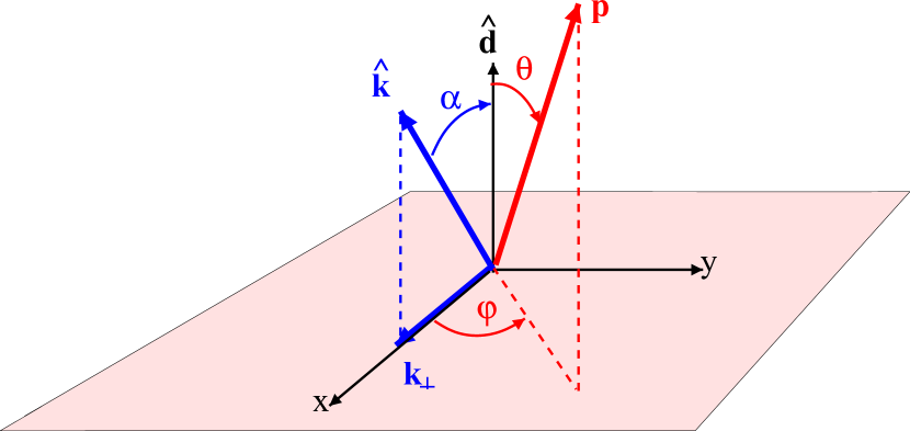
Figure 1: (Color online) For the explicit evaluation of the self-energy we choose our coordinate system such that the $z$ axis points in the direction $\hat{\bm{d}}$ of the dipoles and the $x$ axis lies in the plane spanned by $\hat{\bm{d}}$ and $\hat{\bm{k}}$. We call $\hat{\bm{d}}\cdot\hat{\bm{k}}=\cos\alpha$, ${\bm{k}}_{\bot}=\sin\alpha\hat{\bm{x}}$, and parametrize the integration vector $\bm{p}$ in Eq. (12) as $\bm{p}=p[\cos\theta\hat{\bm{d}}+\sin\theta(\cos\varphi\hat{\bm{x}}+\sin\varphi\hat{\bm{y}})]$.

To first order in the interaction, the irreducible self-energy is given by

$$\Sigma^{(1)}(\bm{k})=\int\frac{d^{3}q}{(2\pi)^{3}}(U_{0}-U_{\bm{q}})f(\epsilon_{\bm{k}+\bm{q}}),$$ (5)

where $f(\epsilon)=[e^{\beta(\epsilon-\mu)}+1]^{-1}$ is the Fermi function at inverse temperature $\beta$ and chemical potential $\mu$, and we have taken the limit $V\rightarrow\infty$ to replace the sum over $\bm{q}$ by an integral. The first-order Hartree and Fock diagrams taken into account in Eq. (5) are shown in Fig. 2 (a).

Figure 2: Relevant Feynman diagrams: (a) first-order Hartree-Fock diagrams; (b) second-order diagrams generated by the self-consistent Hartree-Fock approximation; (c) additional (frequency dependent) second-order diagrams. Here solid lines denote the bare propagator while wavy lines denote the dipole-dipole interaction.

Since the limit ${\bm{q}}\rightarrow 0$ of $U_{\bm{q}}$ is ambiguous, we follow Fregoso et al. Fregoso et al. (2009) and define $U_{0}$ in terms of the angular average of $U_{\bm{q}}$. This amounts to formally setting $U_{0}\rightarrow 0$ so that all Hartree bubbles vanish. We may improve the first-order approximation by replacing $\epsilon_{\bm{k}+\bm{q}}\rightarrow\epsilon_{\bm{k}+\bm{q}}+\Sigma(\bm{k}+\bm{q})$ on the right-hand side of Eq. (5), so that we obtain

$$\Sigma^{\rm HF}(\bm{k})=\int\frac{d^{3}q}{(2\pi)^{3}}(U_{0}-U_{\bm{q}})f\left(\epsilon_{\bm{k}+\bm{q}}+\Sigma^{\rm HF}(\bm{k}+\bm{q})\right),$$ (6)

known as the self-consistent Hartree-Fock approximation. Diagrammatically, this equation amounts to an infinite resummation of perturbation theory, where the bare propagators in the first-order diagrams shown in Fig. 2 (a) are replaced by self-consistent propagators

$$G^{\rm HF}(\bm{k},\omega)=\frac{1}{\omega-\epsilon_{\bm{k}}+\mu-\Sigma^{\rm HF}(\bm{k})}.$$ (7)

The angular dependence of the first-order self-energy $\Sigma^{(1)}(\bm{k})$ can be extracted analytically by means of a suitable rotation of the integration variables. Since we shall use the same procedure for the evaluation of the second-order self-energy, let us explain this in some detail. The dependence of the integral in Eq. (5) on the angular part $\hat{\bm{k}}$ of $\bm{k}$ enters in the form

$$I(\hat{\bm{k}},\hat{\bm{d}})=\int\frac{d^{3}q}{(2\pi)^{3}}A(\hat{\bm{d}}\cdot\hat{\bm{q}})B(\hat{\bm{k}}\cdot{\bm{q}}),$$ (8)

where the functions $A$ and $B$ denote the different factors of the integrand resulting from the substitution of Eq. (4) into Eq. (5). Let us now define rotated integration variables $\bm{p}=e^{\bm{\alpha}\times}\bm{q},$ where we have represented the rotation of a vector $\bm{q}$ around an axis $\hat{\bm{\alpha}}=\bm{\alpha}/|\bm{\alpha}|$ with angle $\alpha=|\bm{\alpha}|$ in terms of an exponentiated cross product,

$$e^{\bm{\alpha}\times}\bm{q}=\hat{\bm{\alpha}}(\hat{\bm{\alpha}}\cdot\bm{q})+\hat{\bm{\alpha}}\times\bm{q}\sin\alpha-\hat{\bm{\alpha}}\times(\hat{\bm{\alpha}}\times\bm{q})\cos\alpha.$$ (9)

Choosing $\bm{\alpha}$ such that the corresponding rotation maps the direction $\hat{\bm{k}}$ into the direction $\hat{\bm{d}}$ of the dipoles (see Fig. 1), we have

$$\hat{\bm{d}}=e^{\bm{\alpha}\times}\hat{\bm{k}},\;\;\;\hat{\bm{\alpha}}=\frac{\hat{\bm{k}}\times\hat{\bm{d}}}{|\hat{\bm{k}}\times\hat{\bm{d}}|},$$ (10)

where $\cos\alpha=k_{\parallel}=\hat{\bm{k}}\cdot\hat{\bm{d}}.$ We may always choose the angle $\alpha$ such that $0\leq\alpha\leq\pi$ and therefore $\sin\alpha=k_{\bot}=|\hat{\bm{k}}\times\hat{\bm{d}}|.$ Next, we use the invariance of the scalar products under rotations and obtain

$$I(\hat{\bm{k}},\hat{\bm{d}})=\int\frac{d^{3}p}{(2\pi)^{3}}A\left((e^{\bm{\alpha}\times}\hat{\bm{d}})\cdot\hat{\bm{p}}\right)B(\hat{\bm{d}}\cdot{\bm{p}}).$$ (11)

With these definitions $e^{\bm{\alpha}\times}\hat{\bm{d}}=\hat{\bm{d}}(\hat{\bm{d}}\cdot\hat{\bm{k}})-{\bm{k}}_{\bot},$ where ${\bm{k}}_{\bot}=\hat{\bm{k}}-\hat{\bm{d}}(\hat{\bm{d}}\cdot\hat{\bm{k}})$ is the component of the unit vector $\hat{\bm{k}}$ perpendicular to $\hat{\bm{d}}$ as shown in Fig. 1. We obtain

$$I(\hat{\bm{k}},\hat{\bm{d}})=\int\frac{d^{3}p}{(2\pi)^{3}}A\left((\hat{\bm{d}}\cdot\hat{\bm{p}})(\hat{\bm{d}}\cdot\hat{\bm{k}})-{\bm{p}}_{\bot}\cdot{\bm{k}}_{\bot}\right)B(\hat{\bm{d}}\cdot{\bm{p}}),$$ (12)

where again ${\bm{p}}_{\bot}=\hat{\bm{p}}-\hat{\bm{d}}(\hat{\bm{d}}\cdot\hat{\bm{p}})$. Using the coordinate system and the spherical coordinates defined in Fig. 1 we arrive at the following expression for the integral (8),

$$I(\hat{\bm{k}},\hat{\bm{d}}) = \frac{1}{(2\pi)^{3}}\int_{0}^{\infty}dpp^{2}\int_{0}^{\pi}d\theta\sin\theta\int_{0}^{2\pi}d\varphi$$ (13)

$$\times A(k_{\parallel}\cos\theta-k_{\bot}\sin\theta\cos\varphi)B(p\cos\theta).\hskip 19.91692pt$$

Applying this to Eq. (5) we find

$$\Sigma^{(1)}(\bm{k}) = -\frac{8\pi d^{2}}{3(2\pi)^{2}}\int_{0}^{\infty}dpp^{2}\int_{0}^{\pi}d\theta\sin\theta$$ (14)

$$\times \int_{0}^{2\pi}\frac{d\varphi}{2\pi}P_{2}(k_{\parallel}\cos\theta-k_{\bot}\sin\theta\cos\varphi)$$

$$\times f\left(\epsilon_{k}+\epsilon_{p}+\frac{kp}{m}\cos\theta\right).$$

The $\varphi$ integration can now be performed,

$$\int_{0}^{2\pi}\frac{d\varphi}{2\pi}P_{2}(k_{\parallel}\cos\theta-k_{\bot}\sin\theta\cos\varphi)=P_{2}(\cos\alpha)P_{2}(\cos\theta),$$ (15)

where we have used $\cos\alpha=k_{\parallel}=\hat{\bm{k}}\cdot\hat{\bm{d}}$. It is convenient to introduce the dimensionless coupling constant

$$u=\nu\frac{8\pi d^{2}}{3}=4\pi\frac{nd^{2}}{E_{F0}}=\frac{4d^{2}mk_{F0}}{3\pi},$$ (16)

where $E_{F0}=k_{F0}^{2}/(2m)$ is the Fermi energy of the noninteracting system, $\nu=mk_{F0}/(2\pi^{2})$ is its density of states at the Fermi energy, and $n=k_{F0}^{3}/(6\pi^{2})$ is the particle density in three dimensions. In the limit of vanishing temperature we obtain

$$\frac{\Sigma^{(1)}(\bm{k})}{\mu} = -\gamma uP_{2}(\cos\alpha)\int_{0}^{\infty}\frac{dpp^{2}}{(\gamma k_{F0})^{3}}\int_{0}^{\pi}d\theta\sin\theta$$ (17)

$$\times P_{2}(\cos\theta)\Theta\left(\mu-\epsilon_{k}-\epsilon_{p}-\frac{kp}{m}\cos\theta\right),$$

where $\Theta(x)$ represents the Heaviside step function. The factor $\gamma=\gamma(u)$ is defined in terms of the ratio between the renormalized chemical potential and the bare Fermi energy,

$$\gamma^{2}=\frac{\mu}{E_{F0}}=\frac{\mu}{k_{F0}^{2}/(2m)}.$$ (18)

As usual, we work at fixed particle density, so that the value of $\mu$ should be adjusted to keep the density constant when the interaction is switched on. The explicit calculation of the renormalized chemical potential will be discussed in Sec. IV.2 where we shall show that $\gamma=1-0.10u^{2}+{\cal{O}}(u^{3})$ [see Eq. (43)], so that to first order in the interaction we may set $\gamma\approx 1$. For convenience we introduce the dimensionless variables $\tilde{k}=k/(\gamma k_{F0})$ and $\tilde{p}=p/(\gamma k_{F0})$; the integrand in Eq. (17) is then independent of $\mu$. Performing the remaining integrations one finally obtains Chan et al. (2010); Fregoso and Fradkin (2010)

$$\frac{\Sigma^{(1)}(\bm{{k}})}{\mu}=-\frac{\gamma u}{3}H^{(1)}(\tilde{k})P_{2}(\hat{\bm{k}}\cdot\hat{\bm{d}}),$$ (19)

where

$$H^{(1)}(\tilde{k}) = \frac{1}{8\tilde{k}^{3}}\biggl{[}-3\tilde{k}+8\tilde{k}^{3}+3\tilde{k}^{5}-\frac{3}{2}\bigl{(}\tilde{k}^{2}-1\bigr{)}^{3}\ln\Bigl{|}\frac{\tilde{k}+1}{\tilde{k}-1}\Bigr{|}\biggr{]}$$

is a positive, continuous function with $H^{(1)}(1)=1$. The first-order result (19) implies that to lowest order in the interaction the Fermi surface is distorted in the direction of the external field which reflects the anisotropy of the interaction. Moreover, the renormalized Fermi velocity acquires an angular dependence. We postpone a more detailed discussion to Sec. IV where we shall also discuss the results obtained in second-order perturbation theory.

III Second-order self-energy

To second order in the interaction, there are totally six diagrams contributing to the self-energy which we show in Fig. 2 (b) and (c). The four diagrams in the group (b) are implicitly taken into account via the Hartree-Fock self-consistency condition in Eq. (6). The contribution of these diagrams can therefore be calculated analytically; together with the first-order contribution (II) we obtain at this level of approximation

$$\frac{\Sigma^{\rm HF}(\bm{{k}})}{\mu}= - \frac{\gamma u}{3}H^{(1)}(\tilde{k})P_{2}(\hat{\bm{k}}\cdot\hat{\bm{d}})+(\gamma u)^{2}\Bigl{[}-\frac{1}{60}H^{(2)}_{0}(\tilde{k})$$ (21)

$$+ \frac{1}{42}H^{(2)}_{2}(\tilde{k})P_{2}(\hat{\bm{k}}\cdot\hat{\bm{d}})-\frac{1}{140}H^{(2)}_{4}(\tilde{k})P_{4}(\hat{\bm{k}}\cdot\hat{\bm{d}})\Bigr{]}$$

$$+ {\cal{O}}(u^{3}),\hskip 19.91692pt$$

where $P_{4}(x)=\frac{1}{8}[35x^{4}-30x^{2}+3]$ is the fourth Legendre polynomial and the functions $H^{(2)}_{n}(\tilde{k})=H^{(2)}_{n}(k/(\gamma k_{F0}))$ are given by

$$H^{(2)}_{0}(\tilde{k}) = \frac{1}{4\tilde{k}}\Bigl{[}10\tilde{k}-6\tilde{k}^{3}+3\bigl{(}\tilde{k}^{2}-1\bigr{)}^{2}\ln\Bigl{|}\frac{\tilde{k}+1}{\tilde{k}-1}\Bigr{|}\Bigr{]},$$ (22a)

$$H^{(2)}_{2}(\tilde{k}) = \frac{1}{8\tilde{k}^{3}}\Bigl{[}6\tilde{k}-4\tilde{k}^{3}+6\tilde{k}^{5}-3\bigl{(}\tilde{k}^{6}-\tilde{k}^{4}-\tilde{k}^{2}+1\bigr{)}$$ (22b)

$$\times \ln\Bigl{|}\frac{\tilde{k}+1}{\tilde{k}-1}\Bigr{|}\Bigr{]},$$

$$H^{(2)}_{4}(\tilde{k}) = \frac{1}{32\tilde{k}^{5}}\Bigl{[}-210\tilde{k}+290\tilde{k}^{3}-30\tilde{k}^{5}-18\tilde{k}^{7}$$

$$+ 3\bigl{(}\tilde{k}^{2}-1\bigr{)}^{2}\bigl{(}3\tilde{k}^{4}+10\tilde{k}^{2}+35\bigr{)}\ln\Bigl{|}\frac{\tilde{k}+1}{\tilde{k}-1}\Bigr{|}\Bigr{]}.$$

Note that these functions are positive and continuous with $H^{(2)}_{n}(1)=1$.

To complete the second-order calculation, we should add the contribution from the two diagrams shown in Fig. 2 (c) which are not taken into account in self-consistent mean-field theory; the total self-energy to second order in the interaction is then given by

$$\Sigma(\bm{k},i\omega)=\Sigma^{\rm{HF}}(\bm{k})+\Sigma^{(2)}(\bm{k},i\omega)+{\cal{O}}(u^{3}),$$ (23)

where $\Sigma^{\rm{HF}}(\bm{k})$ was defined in Eq. (21) and $\Sigma^{(2)}(\bm{k},i\omega)$, representing the contribution of the two diagrams in Fig. 2 (c), is given by

$$\Sigma^{(2)}(\bm{k},i\omega) = -\frac{1}{(\beta V)^{2}}\sum_{Q,Q^{\prime}}U_{\bm{q}}[U_{\bm{q}}-U_{\bm{q}^{\prime}}]G_{0}(K+Q)$$ (24)

$$\times G_{0}(K+Q^{\prime})G_{0}(K+Q+Q^{\prime}),$$

where in the right-hand side $K=(\bm{k},i\omega)$ is a collective label for momentum $\bm{k}$ and fermionic Matsubara frequency $i\omega$, while $Q=(\bm{q},i\bar{\omega})$ and $Q^{\prime}=(\bm{q}^{\prime},i\bar{\omega}^{\prime})$ depend on bosonic Matsubara frequencies $i\bar{\omega}$ and $i\bar{\omega}^{\prime}$. Moreover, $G_{0}(K)=[i\omega-\epsilon_{\bm{k}}+\mu]^{-1}$ is the noninteracting Matsubara Green’s function. The frequency sums in Eq. (24) can be easily carried out. To obtain the retarded self-energy, we then perform the analytic continuation $i\omega\rightarrow\omega+i0^{+}$ to real frequencies and obtain in the limit of vanishing temperature and infinite volume

$$\Sigma^{(2)}(\bm{k},\omega) = \int\frac{d^{3}q}{(2\pi)^{3}}\int\frac{d^{3}q^{\prime}}{(2\pi)^{3}}\frac{1}{2}[U_{\bm{q}}-U_{\bm{q}^{\prime}}]^{2}\frac{\Theta(\xi_{\bm{k}+\bm{q}})\Theta(\xi_{\bm{k}+\bm{q}^{\prime}})\Theta(-\xi_{\bm{k}+\bm{q}+\bm{q}^{\prime}})+\Theta(-\xi_{\bm{k}+\bm{q}})\Theta(-\xi_{\bm{k}+\bm{q}^{\prime}})\Theta(\xi_{\bm{k}+\bm{q}+\bm{q}^{\prime}})}{\omega+i0^{+}-(\xi_{\bm{k}+\bm{q}}+\xi_{\bm{k}+\bm{q}^{\prime}}-\xi_{\bm{k}+\bm{q}+\bm{q}^{\prime}})},\hskip 19.91692pt$$ (25)

where $\xi_{\bm{k}}=\epsilon_{\bm{k}}-\mu$ and we have rewritten the interaction so that the integrand is manifestly symmetric under ${\bm{q}}\leftrightarrow{\bm{q}^{\prime}}$. The dependence of $\Sigma^{(2)}(\bm{k},\omega)$ on the angular part of ${\bm{k}}$ can be extracted analytically by rotating the integration variables $\bm{q}$ and $\bm{q}^{\prime}$ as described in Sec. II; i.e., we introduce $\bm{p}=e^{\bm{\alpha}\times}\bm{q}$ and $\bm{p}^{\prime}=e^{\bm{\alpha}\times}\bm{q}^{\prime}$, where the rotation matrix $e^{\bm{\alpha}\times}$ rotates $\hat{\bm{k}}$ into $\hat{\bm{d}}$. After these transformations we obtain

$$\frac{\Sigma^{(2)}(\bm{k},\omega)}{\mu} = (\gamma u)^{2}\Big{[}\Sigma^{(2)}_{0}(k,\omega)+P_{2}(\hat{\bm{k}}\cdot\hat{\bm{d}})\Sigma^{(2)}_{2}(k,\omega)+P_{4}(\hat{\bm{k}}\cdot\hat{\bm{d}})\Sigma^{(2)}_{4}(k,\omega)\Big{]},$$ (26)

with

$$\Sigma_{n}^{(2)}(k,\omega) = \int_{0}^{\infty}\frac{dpp^{2}}{(\gamma k_{F0})^{3}}\int_{0}^{\infty}\frac{dp^{\prime}p^{\prime 2}}{(\gamma k_{F0})^{3}}\int_{0}^{\pi}d\theta\sin\theta\int_{0}^{\pi}d\theta^{\prime}\sin\theta^{\prime}\int_{0}^{2\pi}\frac{d\phi}{2\pi}A_{n}(\theta,\theta^{\prime},\phi)$$ (27)

$$\times \mu\frac{\Theta(\xi_{k\hat{\bm{d}}+\bm{p}})\Theta(\xi_{k\hat{\bm{d}}+\bm{p}^{\prime}})\Theta(-\xi_{k\hat{\bm{d}}+\bm{p}+\bm{p}^{\prime}})+\Theta(-\xi_{k\hat{\bm{d}}+\bm{p}})\Theta(-\xi_{k\hat{\bm{d}}+\bm{p}^{\prime}})\Theta(\xi_{k\hat{\bm{d}}+\bm{p}+\bm{p}^{\prime}})}{\omega+i0^{+}-(\xi_{k\hat{\bm{d}}+\bm{p}}+\xi_{k\hat{\bm{d}}+\bm{p}^{\prime}}-\xi_{k\hat{\bm{d}}+\bm{p}+\bm{p}^{\prime}})},$$

where $\bm{p}\cdot\bm{p}^{\prime}=pp^{\prime}[\cos\theta\cos\theta^{\prime}+\sin\theta\sin\theta^{\prime}\cos\phi]$. The coefficients $A_{n}(\theta,\theta^{\prime},\phi)$ are defined via the expansion

$$A(\alpha;\theta,\theta^{\prime},\phi) \equiv \int_{0}^{2\pi}\frac{d\varphi}{2\pi}\frac{1}{2}\Bigl{[}P_{2}(\cos\alpha\cos\theta-\sin\alpha\sin\theta\cos\varphi)-P_{2}(\cos\alpha\cos\theta^{\prime}-\sin\alpha\sin\theta^{\prime}\cos(\varphi+\phi))\Bigr{]}^{2}$$ (28)

$$= A_{0}(\theta,\theta^{\prime},\phi)+P_{2}(\cos\alpha)A_{2}(\theta,\theta^{\prime},\phi)+P_{4}(\cos\alpha)A_{4}(\theta,\theta^{\prime},\phi)$$

and are explicitly given by

$$A_{0}(\theta,\theta^{\prime},\phi) = -\frac{3}{80}\Bigl{[}-5+2\cos(\theta+\theta^{\prime})\cos(\theta-\theta^{\prime})+3\cos(2\theta)\cos(2\theta^{\prime})+4\sin(2\theta)\sin(2\theta^{\prime})\cos\phi$$ (29a)

$$+ 4\sin^{2}\theta\sin^{2}\theta^{\prime}\cos(2\phi)\Bigl{]},$$

$$A_{2}(\theta,\theta^{\prime},\phi) = \frac{3}{56}\Bigl{[}1+2\cos(\theta+\theta^{\prime})\cos(\theta-\theta^{\prime})-3\cos(2\theta)(2\theta^{\prime})-2\sin(2\theta)\sin(2\theta^{\prime})\cos\phi$$ (29b)

$$+ 4\sin^{2}\theta\sin^{2}\theta^{\prime}\cos(2\phi)\Bigl{]},$$

$$A_{4}(\theta,\theta^{\prime},\phi) = -\frac{9}{1120}\Bigl{[}-5+4\cos(\theta+\theta^{\prime})\cos(\theta-\theta^{\prime})-35\cos(2\theta+2\theta^{\prime})\cos(2\theta-2\theta^{\prime})+36\cos(2\theta)\cos(2\theta^{\prime})$$ (29c)

$$- 32\sin(2\theta)\sin(2\theta^{\prime})\cos\phi+8\sin^{2}\theta\sin^{2}\theta^{\prime}\cos(2\phi)\Bigl{]}.$$

The factor $\gamma$ is defined in Eq. (18). As in Sec. II we now introduce dimensionless momenta $\tilde{k}=k/(\gamma k_{F0})$, $\tilde{p}=p/(\gamma k_{F0})$, and $\tilde{p}^{\prime}=p^{\prime}/(\gamma k_{F0})$, as well as the dimensionless frequency $\tilde{\omega}=\omega/\mu$. The $\mu$ dependence of the integrand can then be scaled out and the $\tilde{p}^{\prime}$ integration can be performed analytically, with the result

$$\Sigma_{n}^{(2)}({\tilde{k}},{\tilde{\omega}}) = \int_{0}^{\infty}d\tilde{p}\tilde{p}^{2}\int_{0}^{\pi}d\theta\sin\theta\int_{0}^{\pi}d\theta^{\prime}\sin\theta^{\prime}\int_{0}^{2\pi}\frac{d\phi}{2\pi}A_{n}(\theta,\theta^{\prime},\phi)$$ (30)

$$\times \left[\Theta\bigl{(}\tilde{k}^{2}+\tilde{p}^{2}+2\tilde{k}\tilde{p}\cos\theta-1\bigl{)}Q_{12}(\tilde{k},\tilde{\omega};\tilde{p},\theta,\theta^{\prime},\phi)+\Theta\bigl{(}1-\tilde{k}^{2}-\tilde{p}^{2}-2\tilde{k}\tilde{p}\cos\theta\bigl{)}Q_{21}(\tilde{k},\tilde{\omega};\tilde{p},\theta,\theta^{\prime},\phi)\right].\hskip 19.91692pt$$

Here the functions $Q_{ij}(\tilde{k},\tilde{\omega};\tilde{p},\theta,\theta^{\prime},\phi)$ (with $ij=12$ or $ij=21$) are given by

$$Q_{{ij}}(\tilde{k},\tilde{\omega};\tilde{p},\theta,\theta^{\prime},\phi)=\Theta(-r_{i})\Theta(r_{j})\Theta(p^{+}_{j}-m^{a}_{i})F(m^{a}_{i},p^{+}_{j})+\Theta(r_{i})\Theta(r_{j})\Big{[}\Theta(p^{+}_{j}-m^{b}_{i})F(m^{b}_{i},p^{+}_{j})+\Theta(m^{c}_{i}-m^{a}_{i})F(m^{a}_{i},m^{c}_{i})\Big{]},$$

where we have introduced the abbreviations

$$p^{\pm}_{1} = -\tilde{k}\cos\theta^{\prime}\pm\sqrt{r_{1}},$$ (32a)

$$p^{\pm}_{2} = -\tilde{k}\cos\theta^{\prime}-\tilde{p}w\pm\sqrt{r_{2}},$$ (32b)

$$w = \cos\theta\cos\theta^{\prime}+\sin\theta\sin\theta^{\prime}\cos\phi,$$ (32c)

$$r_{1} = 1-\tilde{k}^{2}\sin^{2}\theta^{\prime},$$ (32d)

$$r_{2} = (\tilde{k}\cos\theta^{\prime}+\tilde{p}w)^{2}-\tilde{p}^{2}-2\tilde{k}\tilde{p}\cos\theta-\tilde{k}^{2}+1,\hskip 19.91692pt$$ (32e)

$$m^{a}_{1} = \max(0,p^{-}_{2}),\;\;\;\;\;\;\,\;\;m^{a}_{2}=\max(0,p^{-}_{1}),$$ (32f)

$$m^{b}_{1} = \max(0,p^{-}_{2},p^{+}_{1}),\;\;\;m^{b}_{2}=\max(0,p^{-}_{1},p^{+}_{2}),$$ (32g)

$$m^{c}_{1} = \min(p^{-}_{1},p^{+}_{2}),\;\;\;\;\;\;\,m^{c}_{2}=\min(p^{-}_{2},p^{+}_{1}),$$ (32h)

and the function

$$F(x,y) = -\frac{x-y}{4\tilde{p}^{2}w^{2}}\left[\tilde{p}w(x+y)-\tilde{\omega}+\tilde{k}^{2}-1\right]$$ (33)

$$+\frac{(\tilde{\omega}-\tilde{k}^{2}+1)^{2}}{8\tilde{p}^{3}w^{3}}\ln\left[\frac{\tilde{\omega}+i0^{+}-\tilde{k}^{2}+1+2\tilde{p}wy}{\tilde{\omega}+i0^{+}-\tilde{k}^{2}+1+2\tilde{p}wx}\right].$$

By splitting the complex function $F(x,y)$ into its real and imaginary part, we obtain the real and the imaginary part of the second-order self-energy. We have performed the remaining four-dimensional integration in Eq. (30) numerically using the VEGAS Monte Carlo algorithm from the GNU Scientific Library GSL .

IV Renormalized Fermi surface and quasiparticle properties

IV.1 General definitions

Given the momentum and frequency dependent retarded self-energy $\Sigma(\bm{k},\omega)$, the wavevectors on the renormalized Fermi surface can be obtained from the solution of

$$\epsilon_{\bm{k}_{F}}+\Sigma(\bm{k}_{F},i0^{+})=\mu.$$ (34)

Moreover the effective mass and the quasiparticle residue can be defined in terms of the low-energy expansion of the self-energy around the renormalized Fermi surface,

$$\Sigma(\bm{k}_{F}+\bm{q},\omega) \approx \Sigma(\bm{k}_{F},i0^{+})+\left.\nabla_{\bm{k}}\Sigma(\bm{k},i0^{+})\right|_{\bm{k}=\bm{k}_{F}}\cdot\bm{q}$$ (35)

$$+ \left.\frac{\partial\Sigma(\bm{k}_{F},\omega)}{\partial\omega}\right|_{\omega=i0^{+}}\omega.$$

In this approximation the retarded Green’s function has the quasiparticle form

$$G(\bm{k}_{F}+\bm{q},\omega)\approx\frac{Z_{\bm{k}_{F}}}{\omega+i0^{+}-{\bm{v}}_{\bm{k}_{F}}\cdot\bm{q}},$$ (36)

with the quasiparticle residue

$$Z_{\bm{k}_{F}}=\frac{1}{1-\left.\frac{\partial\Sigma(\bm{k}_{F},\omega)}{\partial\omega}\right|_{\omega=i0^{+}}}$$ (37)

and the renormalized Fermi velocity

$${\bm{v}}_{\bm{k}_{F}}=Z_{\bm{k}_{F}}\left[\frac{\bm{k}_{F}}{m}+\left.\nabla_{\bm{k}}\Sigma(\bm{k},i0^{+})\right|_{\bm{k}=\bm{k}_{F}}\right].$$ (38)

Note that by construction ${\bm{v}}_{\bm{k}_{F}}$ is perpendicular to the renormalized Fermi surface at point $\bm{k}_{F}$. Therefore the information about the direction of the Fermi velocity is redundant if we know the shape of the renormalized Fermi surface and we can restrict ourselves to the calculation of $|{\bm{v}}_{\bm{k}_{F}}|$. The effective mass can be defined by setting

$$|\bm{v}_{\bm{k}_{F}}|=\frac{|\bm{k}_{F}|}{m^{\ast}},$$ (39)

but this obviously does not contain any new information beyond $|\bm{k}_{F}|$ and $|\bm{v}_{F}|$. Because in second-order perturbation theory the self-energy has also an imaginary part, we obtain a broadened spectral function

$$\rho(\bm{k},\omega)=-\frac{1}{\pi}\frac{\text{Im}\Sigma(\bm{k},\omega)}{\left[\omega-\epsilon_{\bm{k}}+\mu-\text{Re}\Sigma(\bm{k},\omega)\right]^{2}+\left[\text{Im}\Sigma(\bm{k},\omega)\right]^{2}}.$$ (40)

IV.2 Renormalized Fermi surface

To begin with, let us calculate the renormalized Fermi surface, which we parametrize by $\bm{k}_{F}=k_{F}(\alpha)\hat{\bm{k}}_{F}$, where $\alpha$ is the angle between $\bm{k}_{F}$ and the direction $\hat{\bm{d}}$ of the dipoles; i.e., $\cos\alpha=\hat{\bm{k}}_{F}\cdot\hat{\bm{d}}$. Substituting the definition $\mu=\gamma^{2}E_{F0}$ introduced in Eq. (18) into the defining equation (34) of the renormalized Fermi surface we obtain

$$\frac{k_{F}(\alpha)}{\gamma k_{F0}}\equiv\tilde{k}_{F}(\alpha)=\sqrt{1-\frac{\Sigma(\tilde{k}_{F}(\alpha)\hat{\bm{k}}_{F},i0^{+})}{\mu}}.$$ (41)

Given our perturbative result for the self-energy we can now iterate Eq. (41) to obtain an expansion of $\tilde{k}_{F}(\alpha)$ in powers of $(\gamma u)$. Since we keep the particle density $n$ fixed, Luttinger’s theorem Luttinger (1960) tells us that the volume of the Fermi surface must not change due to the interaction, so that we can fix the factor $\gamma$ from the condition

$$\left(\gamma k_{F0}\right)^{3}2\pi\int_{0}^{\pi}d\alpha\sin\alpha\int_{0}^{\tilde{k}_{F}(\alpha)}d\tilde{k}\tilde{k}^{2}=\frac{4\pi}{3}k_{F0}^{3},$$ (42)

where we have introduced the rescaled integration variable $\tilde{k}=k/(\gamma k_{F0})$. Substituting the perturbative expression for $\tilde{k}_{F}(\alpha)$ from Eq. (41) into Eq. (42) and expanding the integral to second order in $(\gamma u)$, we determine $\gamma$ to second order in the interaction as

$$\gamma=1-0.10u^{2}+{\cal{O}}(u^{3}).$$ (43)

The reason why there is no term linear in $u$ is that the first-order self-energy is proportional to $P_{2}(\cos\alpha)$ [see Eq. (19)], so that the corresponding first-order contribution to the integral over the Fermi volume vanishes. From Eq. (43) we may then determine the renormalized Fermi surface to second order,

$$\frac{k_{F}(\alpha)}{k_{F0}} = 1+\frac{u}{6}P_{2}(\cos\alpha)-u^{2}\Bigl{[}\frac{1}{180}-0.031P_{2}(\cos\alpha)$$ (44)

$$- 0.016P_{4}(\cos\alpha)\Bigl{]}+{\cal{O}}(u^{3}).$$

The corresponding Fermi surface for $u=1.5$ is shown in Fig. 3.

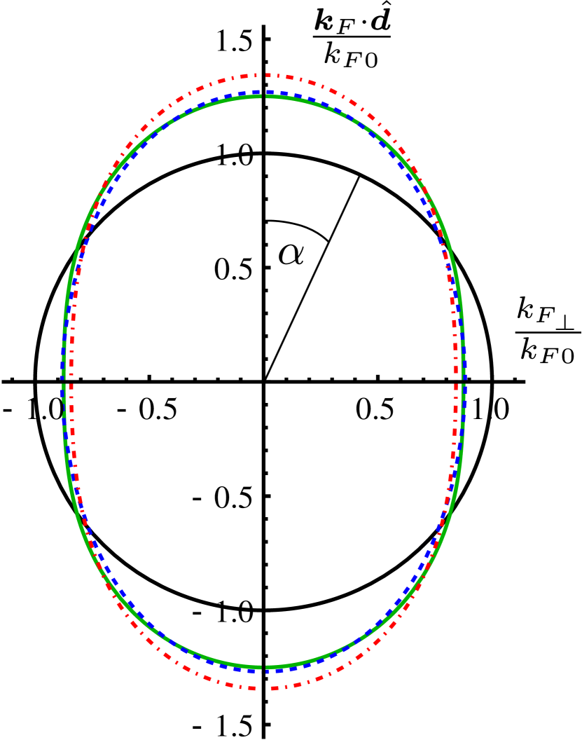
Figure 3: (Color online) Fermi surface of dipolar fermions for $u=1.5$ to first order (solid green), to second order in the self-consistent Hartree-Fock approximation (dashed blue), and to full second order (dot-dashed red) in the interaction. The spherical Fermi surface of the noninteracting system is given as a reference (solid black line). Note that the deformed Fermi surface still has the azimuthal symmetry around the $z$ axis.

Such a large value of the interaction is close to the stability limit of the Fermi liquid state (see Sec. IV.3); in the weak-coupling limit $u\ll 1$ (where our perturbative calculation can be trusted) the second-order correction is barely visible. From Fig. 3 we see that the second-order correction enhances the tendency found in the first-order calculation to distort the Fermi surface along the direction of the dipoles. We also see that the true many-body corrections to the self-energy shown in Fig. 2 (c) have a much stronger effect than the second-order diagrams taken into account via the self-consistent Hartree-Fock approximation. To make contact with the recent experiment by Aikawa et al. [Aikawa et al., 2014b], we show in Fig. 4 how the aspect ratio of the Fermi surface, defined by $k_{F}(0)/k_{F}(\frac{\pi}{2})$, changes in the experimentally relevant range of interactions. Obviously, the second-order correction leads to a slightly larger deviation from the spherical shape of the Fermi surface, but for the experimentally relevant range of interactions the second-order correction is more than an order of magnitude smaller than the first-order result. Hence, for the range of interactions relevant to the experiment by Aikawa et al. [Aikawa et al., 2014b] the deformation of the Fermi surface can be accurately calculated in first order perturbation theory. However, in two dimensions Fermi surface deformations can go first order in a non-analytic way Yamaji et al. (2006); Carr et al. (2010); Slizovskiy et al. (2014). Whether this possibility applies to our three-dimensional system is beyond the scope of this work.

Note that a direct quantitative comparison between our results and the measurements of Aikawa et al. is not meaningful, since they consider dipolar fermions in a trap and argue that first-order interaction corrections due to the time-of-flight expansion cannot be ignored. Taking these effects into account they find good agreement between their Hartree-Fock calculation and the experimental data. Given the smallness of the second-order corrections obtained in our work, it is not surprising that a first-order calculation is sufficient to explain the measurements.

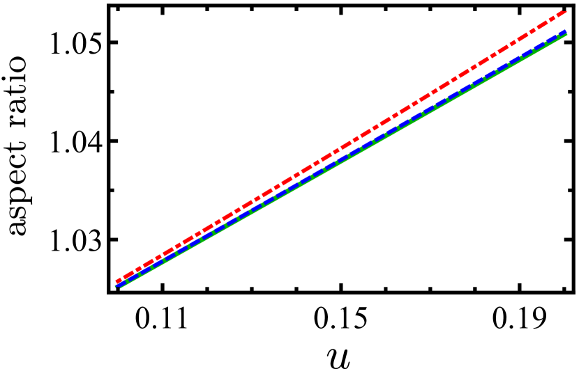
Figure 4: (Color online) Aspect ratio $k_{F}(0)/k_{F}(\frac{\pi}{2})$ of the deformed Fermi surface for values of $u$ which have recently been reached experimentally Aikawa et al. (2014b). The lines correspond to our results to first order (solid green), to second order in the self-consistent Hartree-Fock approximation (dashed blue), and to full second order (dot-dashed red) in the interaction. While the second-order corrections taken into account in the self-consistent Hartree-Fock approximation have practically no effect, the full second-order calculation changes the first-order result for the aspect ratio by about one per mille which is of the same order of magnitude as the experimental uncertainty Aikawa et al. (2014b).

IV.3 Bulk modulus and instability of the normal state

Combining Eqs. (18) and (43) we find the renormalized chemical potential to second order in the interaction,

$$\mu=\gamma^{2}E_{F0}=\frac{k_{F0}^{2}}{2m}[1-0.21u^{2}+{\cal{O}}(u^{3})].$$ (45)

Using the fact that the density is related to the bare Fermi momentum as $n=(k_{F0})^{3}/(6\pi^{2})$ we obtain the bulk modulus to second order in the interaction

$$K=n^{2}\biggl{(}\frac{\partial\mu}{\partial n}\biggr{)}_{V,T}=\frac{2}{3}nE_{F0}\left[1-0.42u^{2}+\mathcal{O}(u^{3})\right].$$ (46)

The fact that the second-order interaction correction to the bulk modulus is negative suggests that for sufficiently large values of the interaction the bulk modulus vanishes and the normal Fermi liquid state becomes unstable in the density-density channel. Indeed, if we use our second-order result (46) to estimate the critical interaction strength $u_{c}$ where $K(u_{c})=0$ we obtain $u_{c}\approx 1.55$. This is significantly lower than the estimate based on the second-order Hartree-Fock result $u^{\rm HF}_{c}=3\sqrt{10/7}\approx 3.6$ [where we neglect the Feynman diagrams in Fig. 2 (c)], while it compares quite well with the result $u^{\rm BG}_{c}\approx 2.1$ obtained by Liu and Yin Liu and Yin (2011) using the Brueckner-Goldstone formalism to second order in $u$. As already mentioned in Sec. I the system may also exhibit other instabilities, e.g., into a biaxial nematic Fregoso et al. (2009) or superfluid Baranov et al. (2002) phase. While we did not look at this possibility in our work, one should note that these instabilities are in principle allowed and may even precede the density-density instability.

IV.4 Quasiparticle residue and Fermi velocity

Inserting our results for the frequency derivative of the self-energy (which we carried out analytically before the numerical integration) into Eq. (37) we obtain for the quasiparticle residue

$$Z_{\bm{k}_{F}} = 1-u^{2}\big{[}0.10+0.029P_{2}(\cos\alpha)$$ (47)

$$\hskip 28.45274pt-0.027P_{4}(\cos\alpha)\big{]}+{\cal{O}}(u^{3}).$$

Similarly, from Eq. (38) we obtain for the modulus of the renormalized Fermi velocity

$$\frac{|{\bm{v}}_{\bm{k}_{F}}|}{v_{F0}} = 1-\frac{u}{12}P_{2}(\cos\alpha)-u^{2}\bigl{[}0.17+0.048P_{2}(\cos\alpha)$$ (48)

$$\hskip 56.9055pt-0.027P_{4}(\cos\alpha)\bigl{]}+{\cal{O}}(u^{3}),$$

where $v_{F0}$ is the bare Fermi velocity. In the upper panel of Fig. 5 we show the quasiparticle residue as a function of the angle $\alpha$ between ${\bm{k}}_{F}$ and the direction $\hat{\bm{d}}$ and the dimensionless interaction $u$ in the range of interactions relevant for the experiment by Aikawa et al. Aikawa et al. (2014b).

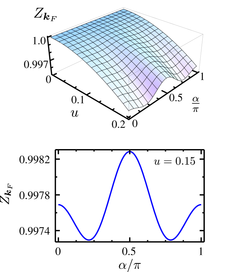
Figure 5: (Color online) Quasiparticle residue $Z_{\bm{k}_{F}}$ of dipolar fermions to second order in the interaction; see Eq. (47). In the upper panel we show $Z_{\bm{k}_{F}}$ as a function of the dimensionless interaction $u=8\pi\nu d^{2}/3$ and the angle $\alpha$ between $\bm{k}_{F}$ and $\hat{\bm{d}}$. In the lower panel we have fixed $u=0.15$ and show the angular dependence of the quasiparticle residue. Note that the value $u=0.15$ lies in the currently accessible experimental range Aikawa et al. (2014b).

Due to the small value of the interaction, the quasiparticle residue is reduced only slightly from unity. In the lower panel of Fig. 5 we show the angular dependence of $Z_{\bm{k}_{F}}$ for fixed interaction $u=0.15$. Interestingly, the value of $Z_{\bm{k}_{F}}$ is smallest if the angle between ${\bm{k}}_{F}$ and the direction $\hat{\bm{d}}$ is close to $\pi/4$ or $3\pi/4$. These local minima are due to the significant $P_{4}(\cos\alpha)$ component in the second-order expression for the quasiparticle residue.

In contrast to the quasiparticle residue, the anisotropy of the renormalized Fermi velocity is for small interactions completely dominated by the first-order correction proportional to $P_{2}(\cos\alpha)$. The renormalized Fermi velocity shown in Fig. 6 is therefore directly related to the angular dependence of the interaction.

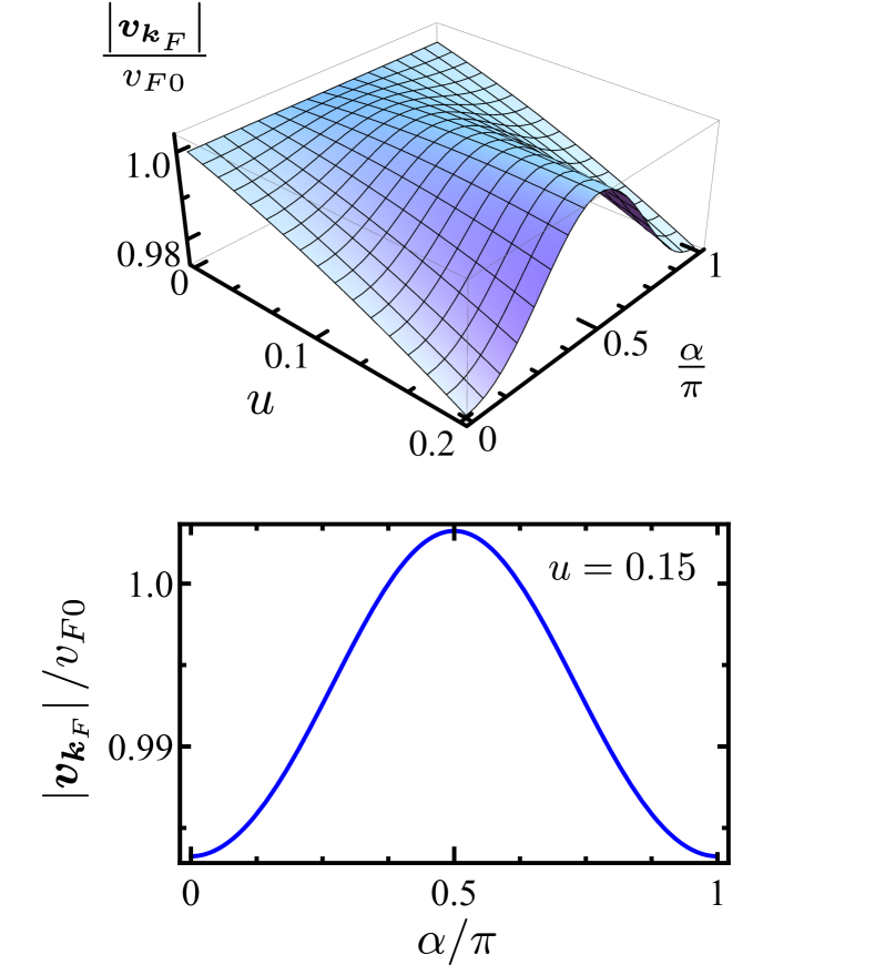
Figure 6: (Color online) Modulus of the renormalized Fermi velocity ${\bm{v}}_{\bm{k}_{F}}$ in units of the bare Fermi velocity to second order in the dimensionless interaction $u$; see Eq. (48). The upper picture shows the behaviour for different interaction strengths, while the lower picture shows the velocity for fixed $u=0.15$ as a function of the angle $\alpha$ between $\bm{k}_{F}$ and $\hat{\bm{d}}$.

If we extrapolate our perturbative result (48) for the renormalized Fermi velocity to large values of the interaction, we find that $|{\bm{v}}_{\bm{k}_{F}}|$ can become negative for $u\geq 2.09$. However, from a similar extrapolation of the perturbative expression for the bulk modulus in Sec. IV.3 we have found that the Fermi liquid phase is unstable for $u\geq 1.55$, so that in the regime where the Fermi liquid phase is stable the Fermi velocity is always positive.

IV.5 Spectral function

Finally, let us present our results for the single-particle spectral function $\rho(\bm{k},\omega)$, which can be obtained by substituting our numerical results for the real and imaginary parts of the retarded second-order self-energy into Eq. (40). In Fig. 7 we show the spectral function $\rho(\bm{k},\omega)$ for wavevectors $\bm{k}$ of the form $\bm{k}=x\bm{k}_{F}$, where the factor $x$ is close to unity. The spectral line shapes can be very well described by Lorentzians whose width shrinks to zero as we approach the Fermi surface, as expected for a Fermi liquid. Interestingly, for momenta above the Fermi surface the width of the spectral line shape (which reflects the damping of the quasiparticles) exhibits a rather strong dependence on the angle $\alpha$ between $\bm{k}_{F}$ and $\hat{\bm{d}}$, while for momenta below the Fermi surface the dependence on $\alpha$ is much weaker.

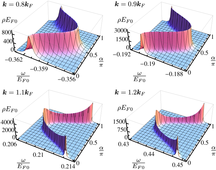
Figure 7: (Color online) Spectral function $\rho(\bm{k},\omega)$ for $u=0.15$ obtained by inserting our numerical results of the second-order self-energy into Eq. (40). The upper pictures show the spectral function for excitations with wavevectors below the renormalized Fermi surface, while the lower pictures give the spectrum for excitations with wavevectors above the renormalized Fermi surface. Note that in the latter case the spectral line shape exhibits a much stronger angular dependence.

V Summary and conclusions

Motivated by a recent experiment by Aikawa et al. Aikawa et al. (2014b) who determined the Fermi surface of a system of ${}^{167}\text{Er}$ atoms via time-of-flight measurements, we have calculated the self-energy $\Sigma(\bm{k},\omega)$ of dipolar fermions in three dimensions to second order in the dipole-dipole interaction. From this we have inferred the deformation of the Fermi surface, the quasiparticle residue, the Fermi velocity, and the spectral function. We have shown that the second-order corrections give rise to a larger elongation of the Fermi surface and a stronger anisotropy of the Fermi velocity than the Hartree-Fock approximation. However, in the experimentally relevant range of interactions the second-order corrections are quite small, so that the Hartree-Fock approximation yields already quantitatively accurate results. On the other hand, if in the future it should be possible to realize dipolar gases where the effective dimensionless interaction $u=8\pi\nu d^{2}/3$ is of the order of unity, then second-order interaction effects become substantial. In particular, the angular dependence of the quasiparticle residue $Z_{\bm{k}_{F}}$ exhibits a significant component proportional to $P_{4}(\cos\alpha)$ which can be directly related to the second-order self-energy.

From our second-order result for the renormalized chemical potential we have also estimated the critical interaction strength for a collapse instability where the Fermi liquid phase becomes unstable. Our estimate $u_{c}\approx 1.55$ is somewhat smaller than the result $u_{c}^{\rm BG}\approx 2.1$ obtained by Liu and Yin Liu and Yin (2011) using the Brueckner-Goldstone formalism to second order in $u$. Note that the critical $u_{c}$ is an order of magnitude larger than the currently experimentally realizable interaction strength. However, given the rapid experimental progress in the field of ultracold quantum gases, we hope that larger values of the dimensionless interaction will be realized in the next few years. In general, we find that the interaction corrections to the quasiparticle properties are rather small for all values of $u$ up to the critical interaction $u_{c}$ where the Fermi liquid exhibits an instability, so that we conclude that the normal phase of dipolar fermions can be viewed as a weakly interacting Fermi liquid.

References

• Chicireanu et al. (2006) R. Chicireanu, A. Pouderous, R. Barbé, B. Laburthe-Tolra, E. Maréchal, L. Vernac, J.-C. Keller,  and O. Gorceix, Phys. Rev. A 73, 053406 (2006).
• Lu et al. (2012) M. Lu, N. Q. Burdick,  and B. L. Lev, Phys. Rev. Lett. 108, 215301 (2012).
• Burdick et al. (2015) N. Q. Burdick, K. Baumann, Y. Tang, M. Lu,  and B. L. Lev, Phys. Rev. Lett. 114, 023201 (2015).
• Aikawa et al. (2014a) K. Aikawa, A. Frisch, M. Mark, S. Baier, R. Grimm,  and F. Ferlaino, Phys. Rev. Lett. 112, 010404 (2014a).
• Aikawa et al. (2014b) K. Aikawa, S. Baier, A. Frisch, M. Mark, C. Ravensbergen,  and F. Ferlaino, Science 345, 1484 (2014b).
• Sage et al. (2005) J. M. Sage, S. Sainis, T. Bergeman,  and D. DeMille, Phys. Rev. Lett. 94, 203001 (2005).
• Deiglmayr et al. (2008) J. Deiglmayr, A. Grochola, M. Repp, K. Mörtlbauer, C. Glück, J. Lange, O. Dulieu, R. Wester,  and M. Weidemüller, Phys. Rev. Lett. 101, 133004 (2008).
• Deiglmayr et al. (2010) J. Deiglmayr, A. Grochola, M. Repp, O. Dulieu, R. Wester,  and M. Weidemüller, Phys. Rev. A 82, 032503 (2010).
• Repp et al. (2013) M. Repp, R. Pires, J. Ulmanis, R. Heck, E. D. Kuhnle, M. Weidemüller,  and E. Tiemann, Phys. Rev. A 87, 010701 (2013).
• Heo et al. (2012) M.-S. Heo, T. T. Wang, C. A. Christensen, T. M. Rvachov, D. A. Cotta, J.-H. Choi, Y.-R. Lee,  and W. Ketterle, Phys. Rev. A 86, 021602 (2012).
• Wu et al. (2012) C.-H. Wu, J. W. Park, P. Ahmadi, S. Will,  and M. W. Zwierlein, Phys. Rev. Lett. 109, 085301 (2012).
• Ospelkaus et al. (2008) S. Ospelkaus, A. Pe’er, K.-K. Ni, J. J. Zirbel, B. Neyenhuis, S. Kotochigova, P. S. Julienne, J. Ye,  and D. S. Jin, Nature Phys. 4, 622 (2008).
• Ni et al. (2008) K.-K. Ni, S. Ospelkaus, M. H. G. de Miranda, A. Pe’er, B. Neyenhuis, J. J. Zirbel, S. Kotochigova, P. S. Julienne, D. S. Jin,  and J. Ye, Science 322, 231 (2008).
• Ospelkaus et al. (2009) S. Ospelkaus, K.-K. Ni, M. H. G. de Miranda, B. Neyenhuis, D. Wang, S. Kotochigova, P. S. Julienne, D. S. Jin,  and J. Ye, Farad. Discuss. 142, 351 (2009).
• Ni et al. (2010) K.-K. Ni, S. Ospelkaus, D. Wang, G. Quéméner, B. Neyenhuis, M. H. G. de Miranda, J. L. Bohn, J. Ye,  and D. S. Jin, Nature 464, 1324 (2010).
• de Miranda et al. (2011) M. H. G. de Miranda, A. Chotia, B. Neyenhuis, D. Wang, G. Quéméner, S. Ospelkaus, J. L. Bohn, J. Ye,  and D. S. Jin, Nature Phys. 7, 502 (2011).
• Baranov (2008) M. A. Baranov, Phys. Rep. 464, 71 (2008).
• Baranov et al. (2012) M. A. Baranov, M. Dalmonte, G. Pupillo,  and P. Zoller, Chem. Rev. 112, 5012 (2012).
• Chan et al. (2010) C.-K. Chan, C. Wu, W.-C. Lee,  and S. Das Sarma, Phys. Rev. A 81, 023602 (2010).
• Yamaguchi et al. (2010) Y. Yamaguchi, T. Sogo, T. Ito,  and T. Miyakawa, Phys. Rev. A 82, 013643 (2010).
• Lu et al. (2013) Z.-K. Lu, S. I. Matveenko,  and G. V. Shlyapnikov, Phys. Rev. A 88, 033625 (2013).
• Góral et al. (2001) K. Góral, B.-G. Englert,  and K. Rza̧żewski, Phys. Rev. A 63, 033606 (2001).
• Miyakawa et al. (2008) T. Miyakawa, T. Sogo,  and H. Pu, Phys. Rev. A 77, 061603 (2008).
• Fregoso et al. (2009) B. M. Fregoso, K. Sun, E. Fradkin,  and B. L. Lev, New J. Phys. 11, 103003 (2009).
• Fregoso and Fradkin (2010) B. M. Fregoso and E. Fradkin, Phys. Rev. B 81, 214443 (2010).
• Ronen and Bohn (2010) S. Ronen and J. L. Bohn, Phys. Rev. A 81, 033601 (2010).
• Baillie and Blakie (2010) D. Baillie and P. B. Blakie, Phys. Rev. A 82, 033605 (2010).
• Baranov et al. (2002) M. A. Baranov, M. S. Mar’enko, V. S. Rychkov,  and G. V. Shlyapnikov, Phys. Rev. A 66, 013606 (2002).
• Bruun and Taylor (2008) G. M. Bruun and E. Taylor, Phys. Rev. Lett. 101, 245301 (2008).
• Cooper and Shlyapnikov (2009) N. R. Cooper and G. V. Shlyapnikov, Phys. Rev. Lett. 103, 155302 (2009).
• Zhao et al. (2010) C. Zhao, L. Jiang, X. Liu, W. M. Liu, X. Zou,  and H. Pu, Phys. Rev. A 81, 063642 (2010).
• Liao and Brand (2010) R. Liao and J. Brand, Phys. Rev. A 82, 063624 (2010).
• Fregoso and Fradkin (2009) B. M. Fregoso and E. Fradkin, Phys. Rev. Lett. 103, 205301 (2009).
• Quintanilla et al. (2009) J. Quintanilla, S. T. Carr,  and J. J. Betouras, Phys. Rev. A 79, 031601 (2009).
• Carr et al. (2009) S. T. Carr, J. Quintanilla,  and J. J. Betouras, Int. J. Mod. Phys. B 23, 4074 (2009).
• Maeda et al. (2013) K. Maeda, T. Hatsuda,  and G. Baym, Phys. Rev. A 87, 021604 (2013).
• Sun et al. (2010) K. Sun, C. Wu,  and S. Das Sarma, Phys. Rev. B 82, 075105 (2010).
• Mikelsons and Freericks (2011) K. Mikelsons and J. K. Freericks, Phys. Rev. A 83, 043609 (2011).
• Parish and Marchetti (2012) M. M. Parish and F. M. Marchetti, Phys. Rev. Lett. 108, 145304 (2012).
• Block and Bruun (2014) J. K. Block and G. M. Bruun, Phys. Rev. B 90, 155102 (2014).
• Matveeva and Giorgini (2012) N. Matveeva and S. Giorgini, Phys. Rev. Lett. 109, 200401 (2012).
• Babadi et al. (2013) M. Babadi, B. Skinner, M. M. Fogler,  and E. Demler, Europhys. Lett. 103, 16002 (2013).
• Baranov et al. (2005) M. A. Baranov, K. Osterloh,  and M. Lewenstein, Phys. Rev. Lett. 94, 070404 (2005).
• Baranov et al. (2008) M. A. Baranov, H. Fehrmann,  and M. Lewenstein, Phys. Rev. Lett. 100, 200402 (2008).
• Zhang and Yi (2010) J.-N. Zhang and S. Yi, Phys. Rev. A 81, 033617 (2010).
• Endo et al. (2010) Y. Endo, T. Miyakawa,  and T. Nikuni, Phys. Rev. A 81, 063624 (2010).
• Kestner and Das Sarma (2010) J. P. Kestner and S. Das Sarma, Phys. Rev. A 82, 033608 (2010).
• Zhang et al. (2011) J.-N. Zhang, R.-Z. Qiu, L. He,  and S. Yi, Phys. Rev. A 83, 053628 (2011).
• Góral et al. (2003) K. Góral, M. Brewczyk,  and K. Rza̧żewski, Phys. Rev. A 67, 025601 (2003).
• Sogo et al. (2009) T. Sogo, L. He, T. Miyakawa, S. Yi, H. Lu,  and H. Pu, New J. Phys. 11, 055017 (2009).
• Lima and Pelster (2010a) A. R. P. Lima and A. Pelster, Phys. Rev. A 81, 021606 (2010a).
• Lima and Pelster (2010b) A. R. P. Lima and A. Pelster, Phys. Rev. A 81, 063629 (2010b).
• Abad et al. (2012) M. Abad, A. Recati,  and S. Stringari, Phys. Rev. A 85, 033639 (2012).
• Babadi and Demler (2012) M. Babadi and E. Demler, Phys. Rev. A 86, 063638 (2012).
• Wächtler et al. (2013) F. Wächtler, A. R. P. Lima,  and A. Pelster, arXiv preprint arXiv:1311.5100  (2013).
• Pikovski et al. (2010) A. Pikovski, M. Klawunn, G. V. Shlyapnikov,  and L. Santos, Phys. Rev. Lett. 105, 215302 (2010).
• Baranov et al. (2011) M. A. Baranov, A. Micheli, S. Ronen,  and P. Zoller, Phys. Rev. A 83, 043602 (2011).
• Zinner et al. (2012) N. T. Zinner, B. Wunsch, D. Pekker,  and D.-W. Wang, Phys. Rev. A 85, 013603 (2012).
• Matveeva and Giorgini (2014) N. Matveeva and S. Giorgini, Phys. Rev. A 90, 053620 (2014).
• Nessi et al. (2014) N. Nessi, A. Iucci,  and M. A. Cazalilla, Phys. Rev. Lett. 113, 210402 (2014).
• Lu and Shlyapnikov (2012) Z.-K. Lu and G. V. Shlyapnikov, Phys. Rev. A 85, 023614 (2012).
• Liu and Yin (2011) B. Liu and L. Yin, Phys. Rev. A 84, 053603 (2011).
• (63) GNU Scientific Library (GSL)http://www.gnu.org/software/gsl/manual/html_node/VEGAS.html.
• Luttinger (1960) J. M. Luttinger, Phys. Rev. 119, 1153 (1960).
• Yamaji et al. (2006) Y. Yamaji, T. Misawa,  and M. Imada, J. Phys. Soc. Jpn. 75, 094719 (2006).
• Carr et al. (2010) S. T. Carr, J. Quintanilla,  and J. J. Betouras, Phys. Rev. B 82, 045110 (2010).
• Slizovskiy et al. (2014) S. Slizovskiy, J. J. Betouras, S. T. Carr,  and J. Quintanilla, Phys. Rev. B 90, 165110 (2014).