First-order decomposition of thermal light in terms of a statistical mixture of pulses

Abstract

We investigate the connection between thermal light and coherent pulses, constructing mixtures of single pulses that yield the same first-order, equal-space-point correlation function as thermal light. We present mixtures involving (i) pulses with a Gaussian lineshape and narrow bandwidths, and (ii) pulses with a coherence time that matches that of thermal light. We characterize the properties of the mixtures and pulses. Our results introduce an alternative description of thermal light in terms of multi-frequency coherent states, valid for the description of broadband linear light-matter interactions. We anticipate our results will be relevant to time-resolved measurements that aim to probe the dynamics of systems as if they were excited by natural thermal light.

I Introduction

The interaction of light with matter triggers fundamental processes in systems as diverse as bulk semiconductors, quantum dots, photovoltaics, and living organisms. The study of these processes requires a detailed understanding of the light used to induce them. Of notable interest is light from the sun, which plays a major role in the primary production of energy on the earth through photosynthesis. While the techniques of ultra-fast spectroscopy are central to studying the dynamics of photo-induced processes, such as the timescales and mechanisms underlying the initial step of photosynthesis in light-harvesting complexes, the interpretation of such experimental results and their relevance to natural excitation conditions has been questioned, due to differences between laser pulses and thermal light Jiang1991a ; Mancal2010a ; Hoki2011a ; Fassioli2012a ; Brumer2012a ; Kassal2013a . In principle, systems such as light-harvesting complexes can be completely characterized using ultra-fast pulses, and their response to thermal-light excitation can then be inferred theoretically. However, understanding the relation of thermal light to pulses of light will make it possible to directly study the photodynamics of processes occurring under more natural excitation conditions by probing the system with ultra-fast pulses and then appropriately averaging the results according to the light decomposition.

In Chenu et al. Chenu2014b , we demonstrated that the state of thermal light cannot be written as a mixture of single broadband coherent states. Yet because the experimental characterization of light cannot be done directly but always involves some interaction with matter, we now focus our attention on states of light that reproduce some of the properties (but not the full density matrix) of thermal light. We start with the first-order correlation function, which characterizes effects of light at the level of a linear light-matter interaction Glauber1963a .

A finite-trace mixture of pulses cannot even yield a first-order, equal-space-point correlation function matching that of thermal light, except in the unphysical limit that the amplitudes of the pulses would diverge as the observation volume $\Omega\to\infty$. But by lifting the requirement of a finite trace and allowing the trace of the density matrix to scale linearly with the observation volume $\Omega$, we can mimic this property of thermal light by a mixture of pulses Chenu2014b . Here we provide the details of how to build these particular mixtures. We investigate the properties of such mixtures, and characterize the pulses that compose them.  After some preliminary considerations in sections IIA and IIB below, in section IIC we first consider a mixture of pulses with a Gaussian lineshape, and find that such a decomposition is only possible for pulses with a FWHM on the order of THz or smaller – almost three orders of magnitude more narrow than what is physically expected from the coherence time of thermal radiation at the temperature of the sun. In section IID we then investigate a mixture without restricting the shape of the spectral distribution. We find a solution given by a family of pulses with a lineshape – and therefore coherence time – that itself mimics that of thermal light.  The mean and spread of the energy and momentum of these pulses is considered in section IIE.  Our conclusions, and comments on the relevance of these studies to problems in linear and nonlinear optics, are presented in section III.

II Matching the first-order correlation function of thermal light

Recall that the density operator of a thermal state of light at temperature $T$, in a normalization volume $V$, is given by $\rho^{\text{th}}=\mathrm{e}^{-\beta H}/\mathrm{Tr}(\mathrm{e}^{-\beta H})$, where $\beta=1/k_{B}T$, with $k_{B}$ Boltzmann’s constant, and $H$ is the field Hamiltonian

$$H=\sum_{\mathbf{k}\lambda}\,\hbar\,\omega_{k}\,\left(A_{\mathbf{k}\lambda}^{\dagger}A_{\mathbf{k}\lambda}+\frac{1}{2}\right),$$ (1)

here expressed in terms of a sum over modes with wavevector $\mathbf{k}$ and polarization state $\lambda$; $A_{\mathbf{k}\lambda}^{\dagger}$ and $A_{\mathbf{k}\lambda}$ are the creation and annihilation operators, defined for discrete values of the wave vector, fulfilling the commutation relation $[A_{\mathbf{k}\lambda},A_{\mathbf{k}^{\prime}\lambda^{\prime}}^{\dagger}]=\delta_{\mathbf{k}\mathbf{k}^{\prime}}\delta_{\lambda\lambda^{\prime}}$. In the coherent state basis, the density matrix is given by the P-representation,

$$\rho^{\text{th}}=\prod_{\mathbf{k}\lambda}\int d^{2}\alpha_{\mathbf{k}\lambda}C(\alpha_{\mathbf{k}\lambda})|\alpha_{\mathbf{k}\lambda}\rangle_{{\mathbf{k}\lambda}}\langle\alpha_{\mathbf{k}\lambda}|_{{\mathbf{k}\lambda}}\,,$$ (2)

where $C(\alpha_{\mathbf{k}\lambda})=\mathrm{e}^{-|\alpha_{\mathbf{k}\lambda}|^{2}/\bar{n}_{\mathbf{k}\lambda}}/(\pi\bar{n}_{\mathbf{k}\lambda})$, and where $\bar{n}_{\mathbf{k}\lambda}$ is the mean photon number in mode $\{\mathbf{k},\lambda\}$. Eq. (2) provides a decomposition of a thermal state in terms of a product of mixtures of monochromatic coherent states $|\alpha_{\mathbf{k}\lambda}\rangle_{{\mathbf{k}\lambda}}=\mathrm{e}^{-\nicefrac{{|\alpha_{\mathbf{k}\lambda}|^{2}}}{{2}}}\sum_{n_{\mathbf{k}\lambda}}\alpha_{\mathbf{k}\lambda}^{n_{\mathbf{k}\lambda}}/\sqrt{n_{\mathbf{k}\lambda}!}\>|n_{\mathbf{k}\lambda}\rangle_{{\mathbf{k}\lambda}}$.

Perhaps surprisingly – or perhaps not, depending on one’s perspective – it is not possible to construct $\rho^{th}$ as a mixture of single broadband coherent states, i.e., pulses Chenu2014b . However, by relaxing the constraint that the trace of the density matrix is finite, we show below how to construct a density matrix from pulses that, while it is not equal to $\rho^{\text{th}}$, still leads to a first-order, equal-space-point correlation function equal to that of thermal light.

II.1 General definition of a pulse

To define a pulse of light it is convenient to consider normalization over all of space.  That is, we quantize the electromagnetic field using annihilation and creation operators, ${a}_{\mathbf{k}\lambda}$ and ${a}_{\mathbf{k\lambda}}^{\dagger}$ respectively, where the helicity $\lambda$ is positive or negative, the wave vector $\mathbf{k}$ ranges continuously, and the commutation relations are $\left[{a}_{\mathbf{k}\lambda},{a}_{\mathbf{k}^{\prime}\lambda^{\prime}}^{\dagger}\right]=\delta(\mathbf{k-k}^{\prime})\delta_{\lambda\lambda^{\prime}}$. We then define a pulse of light as a classical-like state of the electromagnetic with localized energy density, characterized by its nominal position $\mathbf{r}_{\mathrm{o}}$, a spectral distribution $f_{\mathbf{r}_{\mathrm{o}}s;\mathbf{k\lambda}}$, and other parameters  – including those necessary to specify the polarization and the direction of propagation – that we label collectively by $s$. The spectral distribution is normalized such that

$$\sum_{\lambda}\int d\mathbf{k}\;\left|f_{\mathbf{r}_{\mathrm{o}}s;\mathbf{k}\lambda}\right|^{2}=1,$$ (3)

with $d\mathbf{k}=dk_{x}dk_{y}dk_{z}$. To build the pulses, we construct generalized creation operator for a mode defined by the spectral distribution $f_{\mathbf{r}_{\mathrm{o}}s;\mathbf{k\lambda}}$,

$${a}_{\mathbf{r}_{\mathrm{o}}s}^{\dagger}=\sum_{\lambda}\int d\mathbf{k}\;f_{\mathbf{r}_{\mathrm{o}}s;\mathbf{k}\lambda}{a}_{\mathbf{k}\lambda}^{\dagger},$$ (4)

with $\left[{a}_{\mathbf{r}_{\mathrm{o}}s},{a}_{\mathbf{r}_{\mathrm{o}}s}^{\dagger}\right]=1$, and describe a pulse by the quantum state

$$\left|\alpha_{\mathbf{r}_{\mathrm{o}}s}f_{\mathbf{r}_{\mathrm{o}}s}\right\rangle\equiv\mathrm{e}^{\alpha_{\mathbf{r}_{\mathrm{o}}s}{a}_{\mathbf{r}_{\mathrm{o}}s}^{\dagger}-\alpha_{\mathbf{r}_{\mathrm{o}}s}^{\ast}{a}_{\mathbf{r}_{\mathrm{o}}s}}\left|vac\right\rangle,$$ (5)

where $\alpha_{\mathbf{r}_{\mathrm{o}}s}$ is a (complex) amplitude and $\left|vac\right\rangle$ is the vacuum state, and we use $f_{\mathbf{r}_{\mathrm{o}}s}$ to indicate the entire spectral distribution $f_{\mathbf{r}_{\mathrm{o}}s;\mathbf{k\lambda}}$. It is easy to confirm that $\left\langle\alpha_{\mathbf{r}_{\mathrm{o}}s}f_{\mathbf{r}_{\mathrm{o}}s}|\alpha_{\mathbf{r}_{\mathrm{o}}s}f_{\mathbf{r}_{\mathrm{o}}s}\right\rangle=1$.

The positive-frequency part of the (Heisenberg) electric field operator can be written as

$${\mathbf{E}}^{(+)}(\mathbf{r},t)=i\sum_{\lambda}\int d\mathbf{k}\;\sqrt{\frac{\hbar\omega_{k}}{16\pi^{3}\epsilon_{0}}}\mathbf{e}_{\mathbf{k}\lambda}\mathrm{e}^{i\mathbf{k\cdot r}}\mathrm{e}^{-i\omega_{k}t}{a}_{\mathbf{k}\lambda},$$ (6)

where $\omega_{k}=c\left|\mathbf{k}\right|$, and we use the polarization vectors $\mathbf{e}_{\mathbf{k\lambda}}$ for helicity $\lambda$,

$$\begin{split}\mathbf{e}_{\mathbf{k}+}&=-\frac{1}{\sqrt{2}}\left(\hat{\mathbf{e}}_{1\mathbf{k}}+i\,\hat{\mathbf{e}}_{2\mathbf{k}}\right),\\ \mathbf{e}_{\mathbf{k}-}&=\frac{1}{\sqrt{2}}\left(\hat{\mathbf{e}}_{1\mathbf{k}}-i\,\hat{\mathbf{e}}_{2\mathbf{k}}\right),\end{split}$$ (7)

defined from real orthogonal unit vectors, $\hat{\mathbf{e}}_{1\mathbf{k}}$ and $\hat{\mathbf{e}}_{2\mathbf{k}}$, which fulfill $\hat{\mathbf{e}}_{1\mathbf{k}}\times\hat{\mathbf{e}}_{2\mathbf{k}}=\hat{\mathbf{k}}$. The classical expectation value for the electric field in the state $\left|\alpha_{\mathbf{r}_{\mathrm{o}}s}f_{\mathbf{r}_{\mathrm{o}}s}\right\rangle$,

$$\mathcal{E}^{(\mathbf{r}_{\mathrm{o}}s)}(\mathbf{r},t)\equiv\langle\alpha_{\mathbf{r}_{\mathrm{o}}s}f_{\mathbf{r}_{\mathrm{o}}s}|\mathbf{E}^{(+)}(\mathbf{r},t)|\alpha_{\mathbf{r}_{\mathrm{o}}s}f_{\mathbf{r}_{\mathrm{o}}s}\rangle\,,$$ (8)

is then given by (6) with the operator ${a}_{\mathbf{k\lambda}}$ replaced by the complex number $\alpha_{\mathbf{r}_{\mathrm{o}}s}f_{\mathbf{r}_{\mathrm{o}}s;\mathbf{k\lambda}}$,

$$\mathcal{E}^{(\mathbf{r}_{\mathrm{o}}s)}(\mathbf{r},t)=i\sum_{\lambda}\int d\mathbf{k}\;\sqrt{\frac{\hbar\omega_{k}}{16\pi^{3}\epsilon_{0}}}\alpha_{\mathbf{r}_{o}s}f_{\mathbf{r}_{o}s;\mathbf{k}\lambda}\mathbf{e}_{\mathbf{k}\lambda}\mathrm{e}^{i\mathbf{k\cdot r}}\mathrm{e}^{-i\omega_{k}t}{.}$$ (9)

So the states $\left|\alpha_{\mathbf{r}_{\mathrm{o}}s}f_{\mathbf{r}_{\mathrm{o}}s}\right\rangle$ characterizing our pulses are multi-chromatic coherent states, and indeed represents the quantum description of what might be called “classical” pulses Glauber1963a with a bandwidth determined by the spectral distribution $f_{\mathbf{r}_{\mathrm{o}}s;\mathbf{k\lambda}}$. They are “coherent” in the sense that they factorize correlation functions according to ${G}^{(n)(\mathbf{r}_{\mathrm{o}}s)}(\mathbf{r}_{1}{t}_{1}\dots\mathbf{r}_{n}{t}_{n};\mathbf{r}_{{n}+1}{t}_{{n}+1}\dots\mathbf{r}_{2{n}}{t}_{2{n}})=\prod_{j}\left(\mathcal{E}^{(\mathbf{r}_{\mathrm{o}}s)}(\mathbf{r}_{j},{t}_{j})\right)^{\ast}\mathcal{E}^{(\mathbf{r}_{\mathrm{o}}s)}(\mathbf{r}_{j+n},{t}_{j+n})$ for all orders of ${n}$, as defined by Glauber Glauber1963a ; here we use the superscript $(\mathbf{r}_{\mathrm{o}}s)$ on $G$ to identify the state $|\alpha_{\mathbf{r}_{\mathrm{o}}s}f_{\mathbf{r}_{\mathrm{o}}s}\rangle$.  In particular, for such states we have the first-order correlation function

$$G_{ij}^{(1)(\mathbf{r}_{\mathrm{o}}s)} (\mathbf{r}_{1}t_{1};\mathbf{r}_{2}t_{2}){}$$

$$\equiv{} \langle\alpha_{\mathbf{r}_{\mathrm{o}}s}f_{\mathbf{r}_{\mathrm{o}}s}|{E}_{i}^{(-)}(\mathbf{r}_{1},t_{1}){E}_{j}^{(+)}(\mathbf{r}_{2},t_{2})|\alpha_{\mathbf{r}_{\mathrm{o}}s}f_{\mathbf{r}_{\mathrm{o}}s}\rangle$$

$$={} \left(\mathcal{E}_{i}^{(\mathbf{r}_{\mathrm{o}}s)}(\mathbf{r}_{1},{t}_{1})\right)^{\ast}\left(\mathcal{E}_{j}^{(\mathbf{r}_{\mathrm{o}}s)}(\mathbf{r}_{2},{t}_{2})\right),$$ (10)

where subscripts on field labels indicate Cartesian components, i.e. $\mathcal{E}_{i}^{(\mathbf{r}_{\mathrm{o}}s)}(\mathbf{r},{t})=\mathcal{E}^{(\mathbf{r}_{\mathrm{o}}s)}(\mathbf{r},{t})\cdot\mathbf{\hat{i}}$.

We consider families of pulses such that, for a fixed set of properties $s$, the pulses only differ by their nominal position $\mathbf{r}_{\mathrm{o}}$. For such a family of pulses we have

$$f_{\mathbf{r}_{\mathrm{o}}s;\mathbf{k\lambda}}=K(s,\mathbf{k}\lambda)\,\mathrm{e}^{-i\mathbf{k\cdot r}_{\mathrm{o}}},$$ (11)

and the associated $\mathcal{E}^{(\mathbf{r}_{\mathrm{o}}s)}(\mathbf{r},{t})$ depends on $\mathbf{r}$ and $\mathbf{r}_{\mathrm{o}}$ only through its dependence on $(\mathbf{r-r}_{\mathrm{o}})$; we will give particular examples of $K(s,\mathbf{k\lambda)}$ below, but for the moment we keep the function very general.  Nonetheless, we do assume that each member of the family is well localized in space at some nominal time $t=0$, with $G_{ij}^{(1)(\mathbf{r}_{\mathrm{o}}s)}(\mathbf{r}0;\mathbf{r}0)\rightarrow 0$ as $\left|\mathbf{r-r}_{\mathrm{o}}\right|\rightarrow\infty$, and that the integral of $G_{ij}^{(1)(\mathbf{r}_{\mathrm{o}}s)}(\mathbf{r}0;\mathbf{r}0)$ over all space is finite.  Then for fixed $\mathbf{r}$ the integral over all $\mathbf{r}_{\mathrm{o}}$ of $G_{ij}^{(1)(\mathbf{r}_{\mathrm{o}}s)}(\mathbf{r}0;\mathbf{r}0)$ will also be finite.

II.2 Construction of a statistical mixture of pulses

In Chenu et al. Chenu2014b , we suggested the consideration of trace-improper density operators, i.e., with a trace diverging as the observation volume $\Omega\to\infty$. Here we explicitly consider the observation volume spanning all of space, and write $\rho^{\rm imp}$ as

$$\rho^{\mathrm{imp}}=\int ds\int d\mathbf{r}_{\mathrm{o}}\;\bar{p}(s)\left|\alpha_{\mathbf{r}_{\mathrm{o}}s}f_{\mathbf{r}_{\mathrm{o}}s}\right\rangle\left\langle\alpha_{\mathbf{r}_{\mathrm{o}}s}f_{\mathbf{r}_{\mathrm{o}}s}\right|$$ (12)

where the integral over $\mathbf{r}_{\rm o}$ ranges over all of space, where $\bar{p}(s)\geq 0$, and

$$\int ds\;\bar{p}(s)=\frac{1}{\mathcal{V}}.$$ (13)

Here $\mathcal{V}$ is a constant with units of volume. The non-negative distribution $\bar{p}(s)$ has dimension of $[\Omega^{-1}V_{s}^{-1}]$, where $V_{s}$ is the volume of the integration space of the parameters $s$.  The issue we wish to address here is:  How do we build such a mixture of pulses, characterized by $\{\bar{p}(s),f_{\mathbf{r}_{\mathrm{o}}s}\}$, that correctly describes the first order, equal-space-point correlation function of thermal light, $G_{ij}^{(1)\mathrm{th}}(\mathbf{r}t;\mathbf{r}{t^{\prime}})$?  That correlation function is given (Loudon2000 ,Kano1962a ) by

$$G_{ij}^{(1)\mathrm{th}}(\mathbf{r}t;\mathbf{r}{t^{\prime}}) = \mathrm{Tr}\left(\rho^{\mathrm{th}}{E}_{i}^{(-)}(\mathbf{r},t){E}_{j}^{(+)}(\mathbf{r},{t^{\prime}})\right)$$

$$= \delta_{ij}\int_{0}^{\infty}\frac{\hbar ck^{3}}{6\pi^{2}\epsilon_{0}}\frac{\mathrm{e}^{-ick(t^{\prime}-t)}}{\mathrm{e}^{\beta\hbar ck}-1}dk.$$

To proceed, we take the set of parameters $s$ used to define our pulses to include a central wave vector $\mathbf{k}_{\mathrm{o}}=k_{\mathrm{o}}\hat{\mathbf{m}}$ of the pulse, with the unit vector $\mathbf{\hat{m}}$ identifying the main propagation direction, and a unit vector $\hat{\mathbf{n}}$ characterizing the polarization; thus $s=\{k_{\mathrm{o}},\mathbf{\hat{m}},\mathbf{\hat{n}}\}$.  Next we specify a form for $f_{\mathbf{r}_{\mathrm{\mathrm{o}}}s;\mathbf{k\lambda}}$ (11), and describe our pulses by

$$f_{\mathbf{r}_{\mathrm{o}}s;\mathbf{k\lambda}}=\mathcal{N\;}L(\mathbf{k,k}_{\mathrm{\mathrm{o}}})\,(\mathbf{e}_{\mathbf{k\lambda}}^{\ast})\cdot(\mathbf{k\times\hat{n}})\,\mathrm{e}^{-i\mathbf{k\cdot r}_{\mathrm{o}}},$$ (15)

where $L(\mathbf{k,k}_{\mathrm{\mathrm{o}}})$ is a real function, and $\mathcal{N}$ is a normalization constant chosen such that $f_{\mathbf{r}_{\mathrm{\mathrm{o}}}s;\mathbf{k\lambda}}$ is normalized.  The convenience of this form can be most easily seen by looking at the expectation value (9) of the positive-frequency part of the electric field operator $\mathbf{E}^{(+)}(\mathbf{r},t)$ for such a pulse,

$$\mathcal{E}^{(\mathbf{r}_{\mathrm{\mathrm{o}}}s)}(\mathbf{r},t) = i\mathcal{N}\alpha_{\mathbf{r}_{\mathrm{\mathrm{o}}}s}\int d\mathbf{k}\;\sqrt{\frac{\hbar\omega_{k}}{16\pi^{3}\epsilon_{0}}}(\mathbf{k\times\hat{n}})L(\mathbf{k,k}_{\mathrm{\mathrm{o}}})$$ (16)

$$\times\mathrm{e}^{i\mathbf{k\cdot(r-r}_{\mathrm{\mathrm{o}}})}\mathrm{e}^{-i\omega_{k}t}\,,$$

where we have used

$$\sum_{\lambda}(\mathbf{k\times\hat{n})\cdot e}_{\mathbf{k\lambda}}^{\ast}\mathbf{e}_{\mathbf{k\lambda}}=(\mathbf{k\times\hat{n}),}$$ (17)

which holds since $(\mathbf{k\times\hat{n})}$ is necessarily perpendicular to $\mathbf{k}$ and

$$\sum_{\lambda}\mathbf{e}_{\mathbf{k\lambda}}^{\ast}\mathbf{e}_{\mathbf{k\lambda}}=\mathbf{U-\hat{k}\hat{k},}$$ (18)

where $\mathbf{U}$ is the unit dyadic.  Note that while the use of any spectral function $f_{\mathbf{r}_{\mathrm{o}}s;\mathbf{k\lambda}}$ in (9) would lead to a divergenceless expectation value $\mathcal{E}^{(\mathbf{r}_{\mathrm{\mathrm{o}}}s)}(\mathbf{r},t)$, the form (15) leads to an expression (16) for $\mathcal{E}^{(\mathbf{r}_{\mathrm{\mathrm{o}}}s)}(\mathbf{r},t)$ in which the polarization vectors $\mathbf{e}_{\mathbf{k\lambda}}$ do not appear.  Further, we see that $\mathcal{E}^{(\mathbf{r}_{\mathrm{\mathrm{o}}}s)}(\mathbf{r},t)$ is centered in space at $\mathbf{r}_{\mathrm{o}}$, and the direction of the vector field $\mathcal{E}^{(\mathbf{r}_{\mathrm{\mathrm{o}}}s)}(\mathbf{r},t)$ lies exclusively in the plane perpendicular to $\mathbf{\hat{n}}$ such that $\hat{\mathbf{n}}\cdot\mathcal{E}^{(\mathbf{r}_{\mathrm{\mathrm{o}}}s)}(\mathbf{r},t)=0$.  Thus $\mathbf{\hat{n}}$ identifies the polarization of the field $\mathcal{E}^{(\mathbf{r}_{\mathrm{\mathrm{o}}}s)}(\mathbf{r},t)$, in that it defines the direction in which the pulse expectation value has no component.

The correlation function for each pulse is given by (10).  From the definition of $\rho^{\mathrm{imp}}$ in (12), we see that the correlation function for the mixture of pulses is given by the weighted sum of correlation functions for individual pulses. Considering the choice of parameters $s$, we explicitly write the integral over the set of parameters as $\int ds\rightarrow\int dk_{\mathrm{o}}d\mathbf{\hat{m}}d\hat{\mathbf{n}}$. In addition, we assume a uniform distribution over pulse directions $\mathbf{\hat{m}}$ and, for a given $\mathbf{\hat{m}}$, we consider an equal weighting of all $\mathbf{\hat{n}}$ perpendicular to $\mathbf{\hat{m}}$. Thus the probability distribution $\bar{p}(s)$ depends only on the magnitude of the central wave vector, $\bar{p}(s)\rightarrow p(k_{\mathrm{o}})$, and the correlation function for the mixture becomes

$$G_{ij}^{(1)\mathrm{imp}}(\mathbf{r}t;\mathbf{r}t^{\prime})={}\int dk_{\mathrm{o}}d\mathbf{\hat{m}}d\hat{\mathbf{n}}\int d\mathbf{r}_{\mathrm{o}}\>{p}(k_{\mathrm{o}})\,G_{ij}^{(1)(\mathbf{r}_{\mathrm{o}}s)}(\mathbf{r}t;\mathbf{r}t^{\prime})\,.$$ (19)

In the rest of this section, we investigate two different mixtures for which $G_{ij}^{(1)\mathrm{imp}}(\mathbf{r}t;\mathbf{r}t^{\prime})=G_{ij}^{(1)\mathrm{th}}(\mathbf{r}t;\mathbf{r}t^{\prime})$, and provide characteristics of the pulses involved.  We first start with a mixture constrained by adopting a Gaussian form for $L(\mathbf{k,k}_{\mathrm{o}})$, and define the conditions under which the $G_{ij}^{(1)\mathrm{imp}}(\mathbf{r}t;\mathbf{r}t^{\prime})$ that results can represent $G_{ij}^{(1)\rm th}(\mathbf{r}t;\mathbf{r}t^{\prime})$. Considering the restrictions found on the bandwidth of pulses that successfully fulfil this decomposition, we then lift the restriction of $L(\mathbf{k,k}_{\mathrm{o}})$ to a Gaussian and propose another form.

II.3 Mixture of Gaussian-like pulses

We take the pulses to be characterized by a Gaussian form for $L(\mathbf{k,k}_{\mathrm{o}})$, and label all properties related to this particular lineshape with the superscript ‘$g$’. The spectral distribution (15) is given by

$$f_{\mathbf{r}_{\mathrm{o}}s;\mathbf{k\lambda}}^{g}=\mathcal{N}^{g}\mathcal{\;}L^{g}(\mathbf{k,k}_{\mathrm{\mathrm{o}}})\,(\mathbf{e}_{\mathbf{k\lambda}}^{\ast})\cdot(\mathbf{k\times\hat{n}})\,\mathrm{e}^{-i\mathbf{k\cdot r}_{\mathrm{o}}},$$ (20)

where we define the real function

$$L^{g}(\mathbf{k},\mathbf{k}_{\mathrm{o}})=\mathrm{e}^{-\frac{|\mathbf{k}-\mathbf{k}_{\mathrm{o}}|^{2}}{2\sigma^{2}}}.$$ (21)

The normalization condition (3) on $f_{\mathbf{r}_{\mathrm{o}}s;\mathbf{k\lambda}}^{g}$ (11) then leads to the normalization constant:

$$\mathcal{N}^{g}=\left({\pi\sqrt{\pi}\sigma^{3}(k_{\mathrm{o}}^{2}+\sigma^{2})}\right)^{-\frac{1}{2}},$$ (22)

and the expectation value of the positive-frequency part of the electric field in such a pulse (16) is given by

$$\mathcal{E}^{g}(\mathbf{r},t) = i\mathcal{N}^{g}\alpha_{\mathbf{r}_{\mathrm{\mathrm{o}}}s}\int d\mathbf{k}\;\sqrt{\frac{\hbar\omega_{k}}{16\pi^{3}\epsilon_{0}}}(\mathbf{k\times\hat{n}})L^{g}(\mathbf{k,k}_{\mathrm{\mathrm{o}}})$$ (23)

$$\times\mathrm{e}^{i\mathbf{k\cdot(r-r}_{\mathrm{\mathrm{o}}})}\mathrm{e}^{-i\omega_{k}t}\,,$$

where the dependence of $\mathcal{E}^{g}(\mathbf{r},t)$ on $\mathbf{r}_{\mathrm{o}}$ and $s$ is kept implicit.

The first-order correlation function for the mixture (19) of such pulses is

$$\begin{split}G_{ij}^{(1){g}}(\mathbf{r}t;\mathbf{r}t^{\prime})={}&\int dk_{\mathrm{o}}d\mathbf{\hat{m}}d\hat{\mathbf{n}}\int d\mathbf{r}_{\mathrm{o}}\>p(k_{\mathrm{o}})\\ &\times\left(\mathcal{E}_{i}^{g}(\mathbf{r},t)\right)^{\ast}\,\left(\mathcal{E}_{j}^{g}(\mathbf{r},t^{\prime})\right)\,.\end{split}$$ (24)

When expressions (23) for $\mathcal{E}_{i}^{g}(\mathbf{r},t)$ and $\mathcal{E}_{j}^{g}(\mathbf{r},t)$ are substituted into (24) there will be integrals over two wavevector variables, but the integral over $\mathbf{r}_{\mathrm{o}}$ will reduce it to an integral over only one remaining such variable $\mathbf{k}$.  We do the integral over $\mathbf{\hat{n}}$ for a fixed $\mathbf{\hat{m}}$, and then do the integrals over the direction $\mathbf{\hat{m}}$ and the direction of $\mathbf{k}$.  Details are given in Appendix A; the result is that (24) can be written in terms of only integrals over the magnitudes of $\mathbf{k}_{\mathrm{o}}$ and $\mathbf{k}$, $k_{\mathrm{o}}$ and $k$ respectively:

$$\begin{split}G_{ij}^{(1){g}}(\mathbf{r}t;\mathbf{r}(t+\tau))={}&\delta_{ij}|\alpha|^{2}\int_{0}^{\infty}d{k}\int_{0}^{\infty}d{k}_{\mathrm{\mathrm{o}}}\>p({k}_{\mathrm{\mathrm{o}}})\\ \times&\frac{\hbar\,c\,k^{3}}{6\pi^{2}\epsilon_{0}}M({k},{k}_{\mathrm{\mathrm{o}}})\,\mathrm{e}^{-i{c}{k}\tau}\,,\end{split}$$ (25)

with

$$\begin{split}M(k,k_{\mathrm{o}})\equiv&\frac{4\pi^{3}\sqrt{\pi}\sigma}{a(\sigma^{2}+k_{\mathrm{o}}^{2})}\,\left((a^{2}-a+1)\,\mathrm{e}^{-\left(\frac{k-k_{\mathrm{o}}}{\sigma}\right)^{2}}\right.\\ -&\left.(a^{2}+a+1)\,\mathrm{e}^{-\left(\frac{k+k_{\mathrm{o}}}{\sigma}\right)^{2}}\right)\,,\end{split}$$ (26)

where $a=2kk_{\mathrm{o}}/\sigma^{2}$.

We can build such a mixture with a correlation function $G_{ij}^{(1)g}(\mathbf{r}t;\mathbf{r}(t+\tau))$ equal to that of thermal light if there exists a non-negative function $p(k_{\mathrm{o}})$ fulfilling

$$\int_{0}^{\infty}p({k}_{\mathrm{\mathrm{o}}})\,M({k},{k}_{\mathrm{\mathrm{o}}})\,d{k}_{\mathrm{\mathrm{o}}}={}\frac{\bar{n}_{\mathbf{k}\lambda}}{|\alpha|^{2}}\,.$$ (27)

It is possible to search for solutions of (27) numerically, and we find a solution for pulses with a spectral FWHM on the order of THz or smaller, i.e., pulses that are on the order of picoseconds in length or longer. But no physical solutions, with positive definite distributions $p(k_{\mathrm{o}})$, can be found for pulses with a bandwidth as broad as the thermal spectrum, i.e. femtosecond pulses.

These pulses have a surprisingly narrow bandwidth, almost three orders of magnitude narrower than what is physically expected from the coherence time of the thermal radiation. The problem is that the Gaussian shape (21) differs too much from the shape required to guarantee that the norm of the integrand of (II.2) is reproduced. Thus the only way to reproduce the thermal $G^{(1)\rm th}(\mathbf{r}t;\mathbf{r}(t+\tau))$ is to choose the width $\sigma$ in Fourier space so small that, compared with the thermal spectrum, $L^{g}(\mathbf{k},\mathbf{k}_{\mathrm{o}})$ is essentially proportional to a Dirac delta function; then the function $p(k_{\mathrm{o}})$ itself is relied on to capture the shape of that integrand.  Minor modifications of (21) could be considered, such as multiplying or dividing $L^{g}(\mathbf{k,k}_{\mathrm{o}})$ by powers of $k$; but we would expect this conclusion to hold even with such changes.

In an attempt to find a mixture consisting of pulses with a broader bandwidth, we lift the restriction on the shape of the spectral distribution. We find pulses that themselves match the spectrum of thermal light.

II.4 Mixture of pulses with unrestricted line shape: ‘thermal’ pulses

We now investigate a mixture of pulses without initially restricting the shape of the spectral distribution (11). We consider all pulses to have the same lineshape and suppose that the set of parameters $s$ depends on the nominal wave vector $\mathbf{k}_{\mathrm{o}}$ only by depending on its direction, represented again by the unit vector $\hat{\mathbf{m}}$. Each pulse is then characterized by the set of parameters $s=\{\hat{\mathbf{m}},\hat{\mathbf{n}}\}$; consequently $V_{s}$ is dimensionless and $\bar{p}(s)$ has dimension of $\Omega^{-1}$.  In our mixture we will integrate over all possible $\mathbf{\hat{m}}$ and all allowable $\mathbf{\hat{n}}$, and so $\bar{p}(s)\rightarrow p$, a constant.

We label these pulses with the superscript $b$ for ‘broadband’ and specify the spectral distribution (15) by

$$f_{\mathbf{r}_{\mathrm{o}}s;\mathbf{k\lambda}}^{b}=\mathcal{N}^{b}\mathcal{\;}L^{b}(\mathbf{k,k}_{\mathrm{\mathrm{o}}})\,(\mathbf{e}_{\mathbf{k\lambda}}^{\ast})\cdot(\mathbf{k\times\hat{n}})\,\mathrm{e}^{-i\mathbf{k\cdot r}_{\mathrm{o}}}$$ (28)

with

$$L^{b}(\mathbf{k},\mathbf{k}_{\mathrm{o}})=l(k)\,\upsilon(\hat{\mathbf{k}}\cdot\hat{\mathbf{m}}),$$ (29)

where the function $\upsilon(x)$ is chosen to characterize the spread in the direction of wave vectors in the pulse and should be peaked at $x=1$ for $\hat{\mathbf{m}}$ to represent the nominal direction of propagation of the pulse; the function $l(k)$ is now relied on to help capture the shape of the norm of the integrand in (II.2).  The normalization condition (3) on $f_{\mathbf{r}_{\mathrm{o}}s;\mathbf{k}\lambda}$ leads to the normalization constant

$$\mathcal{N}^{b}=\left[\pi(C_{0}+C_{2})\int_{0}^{\infty}k^{4}l(k)^{2}dk\right]^{-\frac{1}{2}},$$ (30)

where

$$C_{n}=\int_{-1}^{1}dx\,\,x^{n}\upsilon^{2}(x),$$ (31)

and the expectation value of the positive-frequency part of the electric field in such a pulse (16) is given by

$$\begin{split}\mathcal{E}^{b}(\mathbf{r},t)=&i\mathcal{N}^{b}\alpha_{\mathbf{r}_{\mathrm{\mathrm{o}}}s}\int d\mathbf{k}\;\sqrt{\frac{\hbar\omega_{k}}{16\pi^{3}\epsilon_{0}}}(\mathbf{k\times\hat{n}})L^{b}(\mathbf{k,k}_{\mathrm{\mathrm{o}}})\\ &\times\mathrm{e}^{i\mathbf{k\cdot(r-r}_{\mathrm{\mathrm{o}}})}\mathrm{e}^{-i\omega_{k}t}\,,\end{split}$$ (32)

where the dependence of $\mathcal{E}^{b}(\mathbf{r},t)$ on $\mathbf{r}_{\mathrm{o}}$ and $s$ is kept implicit.

The first-order, equal-space-point correlation function for such a mixture of pulses is

$$G_{ij}^{(1){b}}(\mathbf{r}t;\mathbf{r}t^{\prime})={}\int d\hat{\mathbf{m}}d\hat{\mathbf{n}}\int d\mathbf{r}_{\mathrm{o}}\>p\left(\mathcal{E}_{i}^{b}(\mathbf{r},t)\right)^{\ast}\,\left(\mathcal{E}_{j}^{b}(\mathbf{r},t^{\prime})\right)\,.$$ (33)

As in the mixture of Gaussian pulses, when expressions for $\mathcal{E}_{i}^{b}(\mathbf{r},t)$ and $\mathcal{E}_{j}^{b}(\mathbf{r},t)$ are substituted into (33) there will be integrals over two wavevector variables, but the integral over $\mathbf{r}_{\mathrm{o}}$ will reduce it to an integral over only one remaining such variable $\mathbf{k}$.  The integrals over $\mathbf{\hat{n}}$, $\mathbf{\hat{m}}$, and $\mathbf{\hat{k}}$ can then be done, as detailed in Appendix B, and we find

$$\begin{split}G_{ij}^{(1){b}}(\mathbf{r}t;\mathbf{r}(t+\tau))=&\delta_{ij}\frac{p|\alpha|^{2}}{\int_{0}^{\infty}k^{4}l(k)^{2}dk}\frac{4\pi^{2}}{3\epsilon_{0}}\\ &\times\int_{0}^{\infty}\hbar ck^{5}l(k)^{2}\mathrm{e}^{-ick\tau}dk\,.\end{split}$$ (34)

Imposing the condition $G_{ij}^{(1){b}}(\mathbf{r}t;\mathbf{r}(t+\tau))=G_{ij}^{(1)\mathrm{th}}(\mathbf{r}t;\mathbf{r}(t+\tau))$ yields the condition

$$l(k)=k^{-1}(\mathrm{e}^{\beta\hbar ck}-1)^{-\frac{1}{2}},$$ (35)

with then

$$p|\alpha|^{2}=\frac{1}{8\pi^{4}}\int_{0}^{\infty}\frac{k^{2}}{\mathrm{e}^{\beta\hbar ck}-1}dk=\frac{4\zeta(3)}{\pi^{4}(\beta c\hbar)^{3}}.$$ (36)

This mixture consists of pulses that only differ in their position in space, their propagation direction, and their polarization; they are weighted identically. The coherence time of the pulse, as determined by its spectral FWHM, is the same as thermal light, which is approximatively $1.3$ fs for $T=5777$ $K$. The pulse energy is restricted by the condition that the product $p|\alpha|^{2}$, where recall $|\alpha|^{2}$ corresponds to the average number of photons in a coherent state, is fixed.

Because of the link of their spectrum to the thermal spectrum, we refer to these pulses as “thermal pulses”.

II.5 Properties of the thermal pulses

In this section we consider some elementary properties of these thermal pulses, represented by kets (5) $\left|\alpha_{\mathbf{r}_{\mathrm{o}}s}f_{\mathbf{r}_{\mathrm{o}}s}^{b}\right\rangle$, in the special case where the elements (15) of $f_{\mathbf{r}_{\mathrm{o}}s}^{b}$ are specified by $L^{b}$ (29) and $\mathcal{N}^{b}$ (30).  Since these are the only pulses we consider in this section we avoid clutter in the notation by writing these kets simply as $\left|\alpha f\right\rangle$.

The operator characterizing the energy above the vacuum is

$$\mathfrak{E}=\sum_{\lambda}\int d\mathbf{k\;}\hbar\omega_{k}n_{\mathbf{k}\lambda},$$ (37)

where $n_{\mathbf{k\lambda}}=a_{\mathbf{k\lambda}}^{\dagger}a_{\mathbf{k}\lambda}$, and so the expectation value of the energy of one of our pulses is easily found to be,

$$\begin{split}\left\langle\mathfrak{E}\right\rangle=&\sum_{\lambda}\int d\mathbf{k}\langle\alpha f|\hbar\omega_{k}{n}_{\mathbf{k}\lambda}|\alpha f\rangle\\ =&\hbar c|\alpha|^{2}\frac{\int_{0}^{\infty}k^{5}l(k)^{2}dk}{\int_{0}^{\infty}k^{4}l(k)^{2}dk}\,,\end{split}$$ (38)

and for a lineshape specified by $l(k)$ (35), we find

$$\left\langle\mathfrak{E}\right\rangle=\frac{\pi^{4}}{30\zeta(3)}k_{B}T|\alpha|^{2},$$ (39)

giving $\left\langle\mathfrak{E}\right\rangle=1.34|\alpha|^{2}$ $eV$ at $T=5777$ $K$.  As expected, the energy of the pulse depends on the amplitude of the coherent state $|\alpha|$. This amplitude can in principle be chosen arbitrarily, and the mixture will yield an equal-space-point, first-order correlation function equivalent to that of thermal light provided that the product $p|\alpha|^{2}$ of $|\alpha|^{2}$ with the weighting density $p$ is given by (36). This condition also ensures that such statistical mixture has the same energy density and photon density as thermal light.  The spread in energy of the thermal pulse can be characterized by $\langle\sigma_{\mathfrak{E}}\rangle=\sqrt{\langle\mathfrak{E}^{2}\rangle-\langle\mathfrak{E}\rangle^{2}}$, which is given by

$$\begin{split}\langle\sigma_{\mathfrak{E}}\rangle=&\left((\hbar c)^{2}|\alpha|^{2}\frac{\int_{0}^{\infty}k^{6}l(k)^{2}dk}{\int_{0}^{\infty}k^{4}l(k)^{2}dk}\right)^{\frac{1}{2}}\\ =&\sqrt{\frac{12\zeta(5)}{\zeta(3)}}|\alpha|\,k_{B}T,\end{split}$$ (40)

with details given in Appendix B; we find $\langle\sigma_{\mathfrak{E}}\rangle=1.608\left|\alpha\right|$ $eV$ at $T=5777$ $K$.

While thermal light has no directionality and is isotropic MandelWolfBook , each of our thermal pulses has a mean direction of propagation.  We can characterize it by identifying the average momentum of the pulse.  The momentum operator is

$$\mathcal{P}=\sum_{\lambda}\int d\mathbf{k\;\hbar k\;}n_{\mathbf{k}\lambda},$$ (41)

and the average momentum of a thermal pulse is given by

$$\begin{split}\left\langle\mathcal{P}\right\rangle=&\sum_{\lambda}\int d\mathbf{k}\langle\alpha f|\hbar\mathbf{k}\,n_{\mathbf{k}\lambda}|\alpha f\rangle\\ =&\hbar|\alpha|^{2}\left(\frac{C_{1}+C_{3}}{C_{0}+C_{2}}\right)\frac{\int_{0}^{\infty}k^{5}l(k)^{2}dk}{\int_{0}^{\infty}k^{4}l(k)^{2}dk}\hat{\mathbf{m}}\,\\ =&\frac{C_{1}+C_{3}}{C_{0}+C_{2}}\frac{\pi^{4}}{30\zeta(3)}\frac{k_{B}T}{c}|\alpha|^{2}\hat{\mathbf{m}},\end{split}$$ (42)

where in the last line we have used (35), and details are presented in Appendix B.  As expected, the average momentum is along the mean propagation direction $\hat{\mathbf{m}}$. We can push the evaluation further by assuming a particular form for $\upsilon(x)$, which should be defined on $[-1:1]$ and is peaked at $x=1$; we take

$$\upsilon(x)=\theta(x)\theta(1-x)\mathrm{e}^{-(x-1)^{2}/\gamma^{2}},$$ (43)

where $\theta(x)$ is the Heaviside function, and the smaller the dimensionless parameter $\gamma$ the more the propagation of momentum in the pulse is centered about $\mathbf{\hat{m}}$.  Numerically evaluating the integrals for $\gamma=0.1$ gives $\left\langle\mathcal{P}\right\rangle\approx 1.3$ $|\alpha|^{2}\hat{\mathbf{m}}$ $eV/c$. This remains almost constant for $\gamma$ in the range $\left[0.01;0.1\right]$. We have verified that we obtain similar behaviour with different forms for $\upsilon(x)$.

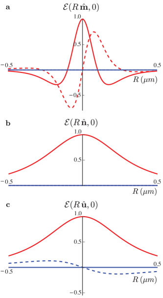
Figure 1: Real (dashed lines) and imaginary (plain lines) parts of the positive-frequency part of the electric field components $\mathcal{E}_{u}(R\,\hat{\mathbf{i}},0)$ (red), $\mathcal{E}_{m}(R\,\hat{\mathbf{i}},0)$ (blue) at position $\mathbf{R}\cdot\hat{\mathbf{i}}$ along the system coordinates $\hat{\mathbf{i}}\equiv\hat{\mathbf{m}}$ (a), $\hat{\mathbf{n}}$ (b) and $\hat{\mathbf{u}}$ (c).

The variance in momentum is characterized by the dyadic $\langle\sigma_{\mathcal{P}}\rangle^{2}=\left\langle\mathcal{PP}\right\rangle-\left\langle\mathcal{P}\right\rangle\left\langle\mathcal{P}\right\rangle$. The strategy for evaluating this is sketched in Appendix B; the result is

$$\begin{split}\langle\sigma_{\mathcal{P}}\rangle^{2}&=\hbar^{2}|\alpha|^{2}\frac{\pi}{4}\mathcal{N}^{2}\int_{0}^{\infty}dk\>k^{6}l(k)^{2}\Big{(}2(C_{4}+C_{2})\mathbf{\hat{m}\hat{m}}\\ &+(C_{0}+2C_{2}-3C_{4})\hat{\mathbf{n}}\hat{\mathbf{n}}+(3C_{0}-2C_{2}-C_{4})\hat{\mathbf{u}}\hat{\mathbf{u}}\Big{)}.\end{split}$$ (44)

Taking (43) with $\gamma=0.1$ and $T=5777$ $K$, for example, we find

$$\langle\sigma_{\mathcal{P}}\rangle^{2}\approx 1.19\left|\alpha\right|^{2}(\mathbf{\hat{m}}\mathbf{\hat{m}}+0.079\mathbf{\hat{n}\hat{n}}+0.084\mathbf{\hat{u}\hat{u}})\>(eV/c)^{2}.$$ (45)

Yet regardless of the temperature $T$ or the form of $v(x)$, since the vectors $\mathbf{\hat{m}}$, $\mathbf{\hat{n}}$, and $\mathbf{\hat{u}}$ are mutually orthogonal we can take the square root of (44) by simply taking the square root of each of the components.  In the special case of (45) we find

$$\langle\sigma_{\mathcal{P}}\rangle\approx 1.09\left|\alpha\right|\left(\mathbf{\hat{m}\hat{m}}+0.28\mathbf{\hat{n}\hat{n}}+0.29\mathbf{\hat{u}\hat{u}}\right)\;eV/c.$$ (46)

The largest spread of momentum is in the direction $\mathbf{\hat{m}}$ the pulse is nominally propagating; the spreads in the other two directions are almost but not identically the same.

Finally, while the energy density of thermal radiation is uniform, our pulses are localized in space.  In Appendix B we give the details for calculating the expectation value (32) of the positive-frequency part of the electric field.  Since this quantity depends only on $\mathbf{r-r}_{\rm o}\equiv\mathbf{R}$ we relabel the left-hand-side of (32) as $\mathcal{E}\left(\mathbf{R},t\right)$, where the pulse is further identified by the direction $\mathbf{\hat{m}}$ of the expectation value of its momentum and the unit vector $\mathbf{\hat{n}}$.  Since the electric field in the pulse has no component in the $\mathbf{\hat{n}}$ direction, the nonvanishing components will only be those along $\mathbf{\hat{m}}$ $\left(\mathcal{E}_{m}\left(\mathbf{R},t\right)\right)$ and along $\mathbf{\hat{u}=\hat{m}\times\hat{n}}$ $\left(\mathcal{E}_{u}\left(\mathbf{R},t\right)\right)$,

$$\mathcal{E}\left(\mathbf{R},t\right)=\mathcal{E}_{u}\left(\mathbf{R},t\right)\,\hat{\mathbf{u}}+\mathcal{E}_{m}\left(\mathbf{R},t\right)\,\hat{\mathbf{m}}.$$ (47)

In Fig. 1 we show the dependence of the electric field components as a function of the distance to the centre of the pulse $R\equiv|\mathbf{r}-\mathbf{r}_{\mathrm{o}}|$. For the figure, we chose $\upsilon(x)$ with a Gaussian shape and $\gamma=0.1$, and put $\alpha=1$. We have investigated the use of shapes different than (43) for $\upsilon(x)$, e.g. $\upsilon(x)=\theta(x)\theta(1-x)\,(1-(x-1)^{2})$, and find that the shape of the electric field is not significantly different for these different $\upsilon(x)$ functions, as long as they are peaked at $x=1$.  From (47) we can easily construct an intensity function,

$$I(\mathbf{R},t)=|\mathcal{E}_{u}\left(\mathbf{R},t\right)|^{2}+|\mathcal{E}_{m}\left(\mathbf{R},t\right)|^{2}.$$ (48)

In Fig. 2 we illustrate the region of space for which the intensity is half of its maximum value, and gives the contour plots in 3D space.

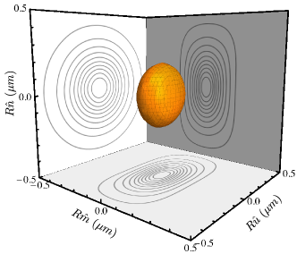
Figure 2: Contour plots of the intensity for the ‘thermal’ pulse (Eq. 48). The 3D zone delimitates the half maximum region.

III Conclusions

Much of the intuition of researchers in optical physics deals with how different states of light are related to each other. Thermal light is well represented by a mixture of tensor products of coherent states describing monochromatic radiation, i.e., continuous waves.  Yet broadband coherent states, i.e., pulses, are central to resolving the dynamics of physical processes. The relation between the two states of light involved here is especially relevant to the study of biological systems such as photosynthetic complexes, which under natural conditions are excited by thermal light, but which are probed in the laboratory with ultra-fast pulses.

In previous work Chenu2014b we showed that thermal light cannot be represented as an incoherent mixture of pulses, in contradiction to the intuition of at least some. Here we showed that the intuition can be maintained if interest is restricted to first-order, equal-space-point correlation functions representative of linear light-matter interaction. We presented two families of pulses, mixtures of which can be used to reproduce the features of the linear interaction of matter with thermal light: (i) pulses with a Gaussian lineshape, with surprisingly narrow bandwidths, (ii) and ”thermal” pulses, with the coherence time of thermal light. In each case the density operator describing the mixture of pulses must be improper, in that its trace is not unity but rather scales with the volume containing the radiation.

The decompositions presented in this paper may prove to be helpful conceptual tools, and useful in some calculations where localized pulses are easier to treat than radiation extending over all space. We also note that while thermal light is often used as a proxy for sunlight, thermal light and sunlight are strikingly different in that sunlight carries momentum while thermal light does not.  So the kind of decompositions we present here might be of use in constructing mixtures to properly represent sunlight.

The conclusion of our earlier work Chenu2014b of course remains: Nonlinear light-matter interactions involving thermal light, described by higher-order correlation functions, cannot in general be described with the aid of mixtures of single pulses of the type presented in this paper. Yet further work is required to investigate the existence of regimes where the use of such a mixture may be at least approximately valid.   This should help in the development of conceptual and calculational tools for understanding and designing nonlinear optical experiments to study excitation by thermal light.

Appendix A First-order correlation function for Gaussian-like pulses

We present here the details of the calculation for the first-order correlation function of the trace-improper mixture composed of pulses with Gaussian lineshape (24).  In addition to the system of coordinates $\{\hat{\mathbf{e}}_{1\mathbf{k}},\hat{\mathbf{e}}_{2\mathbf{k}},\hat{\mathbf{k}}\}$, it is useful to have two sets of three mutually orthogonal unit vectors available for the derivations here and in the following appendices, and we illustrate them in Fig. (3).  One of our sets is $\left\{\mathbf{\hat{e}}_{1\mathbf{m}},\mathbf{\hat{e}}_{2\mathbf{m}},\mathbf{\hat{m}}\right\}$, where $\mathbf{\hat{m}}$ identifies the direction of $\mathbf{k}_{\mathrm{o}}$ and $\mathbf{\hat{e}}_{1\mathbf{m}}$ and $\mathbf{\hat{e}}_{2\mathbf{m}}$ are two unit vectors orthogonal to each other and to $\mathbf{\hat{m}}$, such that $\hat{\mathbf{e}}_{1\mathbf{m}}\times\hat{\mathbf{e}}_{2\mathbf{m}}=\hat{\mathbf{m}}$.  The pulses $\mathcal{E}_{i}^{g}(\mathbf{r},t)$, given by (23), also involve the vector $\mathbf{\hat{n}}$, which is perpendicular to $\mathbf{\hat{m}}$.  It lies in the plane of $\mathbf{\hat{e}}_{1\mathbf{m}}$ and $\mathbf{\hat{e}}_{2\mathbf{m}}$, and we specify it as

$$\hat{\mathbf{n}}=\hat{\mathbf{e}}_{1\mathbf{m}}\cos\Psi+\hat{\mathbf{e}}_{2\mathbf{m}}\sin\Psi.$$ (49)

Our second set of unit vectors is $\left\{\mathbf{\hat{n},\hat{u},\hat{m}}\right\}$ where $\mathbf{\hat{u}}\equiv$ $\mathbf{\hat{m}\times\hat{n}}$.

Figure 3: Representation of selected vectors and angles used in the derivations. The two sets of mutually orthogonal unit vectors $\{\hat{\mathbf{e}}_{1\mathbf{m}},\hat{\mathbf{e}}_{2\mathbf{m}},\hat{\mathbf{m}}\}$ and $\{\hat{\mathbf{n}},\hat{\mathbf{u}},\hat{\mathbf{m}}\}$ each form a direct orthonormal system. The centre is at position $r_{\mathrm{o}}$.

We are now ready to begin.  Once the expression for $\mathcal{E}_{i}^{\mathrm{g}}(\mathbf{r},t)$ is used in (24), the integration over the positions $\mathbf{r}_{\mathrm{o}}$ of the pulses can be done immediately using $\int\mathrm{e}^{i(\mathbf{k}^{\prime}-\mathbf{k})\cdot(\mathbf{r}-\mathbf{r}_{\mathrm{o}})}d\mathbf{r}_{\mathrm{o}}=\left(2\pi\right)^{3}\delta(\mathbf{k}-\mathbf{k}^{\prime})$, we find

$$\begin{split}G_{ij}^{(1){g}}(\mathbf{r}t;\mathbf{r}t^{\prime})=(2\pi)^{3}|i\alpha\mathcal{N}^{g}|^{2}\int\,d\mathbf{k}_{\mathrm{o}}\,d\mathbf{k}\,p(k_{\mathrm{o}})\,\frac{\hbar\,c\,k}{16\pi^{3}\epsilon_{0}}\mathrm{e}^{-\frac{|\mathbf{k}-\mathbf{k}_{\mathrm{o}}|^{2}}{\sigma^{2}}}\mathrm{e}^{-{i}\omega_{k}(t^{\prime}-t)}T_{ij}(\mathbf{k,\hat{m}}),\end{split}$$ (50)

where

$$T_{ij}(\mathbf{k,\hat{m}}) = \int_{0}^{2\pi}d\Psi\left(\hat{\mathbf{i}}\cdot(\mathbf{k}\times\hat{\mathbf{n}})\right)\,\left(\hat{\mathbf{j}}\cdot(\mathbf{k}\times\hat{\mathbf{n}})\right)$$

$$= \varepsilon_{i\eta\mu}\varepsilon_{j\sigma\nu}k_{\eta}k_{\sigma}\int_{0}^{2\pi}d\Psi\;n_{\mu}n_{\nu}$$

$$= \pi\varepsilon_{i\eta\mu}\varepsilon_{j\sigma\nu}k_{\eta}k_{\sigma}\left(\delta_{\mu\nu}-m_{\mu}m_{\nu}\right)$$

$$= \pi\left(\delta_{ij}k^{2}-k_{i}k_{j}\right)-\pi\varepsilon_{i\eta\mu}\varepsilon_{j\sigma\nu}k_{\eta}k_{\sigma}m_{\mu}m_{\nu}\,.$$

In the first line of (A) we have written the integral $d\mathbf{\hat{n}}$ appearing in (24) as an integral $d\Psi$, with $\Psi$ varying from $0$ to $2\pi$; in the second line we have introduced the Levi-Civita tensor ($\varepsilon_{\alpha\beta\gamma}=1$ if $\{\alpha,\beta,\gamma\}$ is a cyclic permutation, $-1$ if the permutation is anti-cyclic, and 0 if any two indices are equal) to write the cross products; in the third line we have used (49) to evaluate

$$\int_{0}^{2\pi}d\Psi\;\mathbf{\hat{n}\hat{n}} = \pi(\hat{\mathbf{e}}_{1\mathbf{m}}\hat{\mathbf{e}}_{1\mathbf{m}}+\hat{\mathbf{e}}_{2\mathbf{m}}\hat{\mathbf{e}}_{2\mathbf{m}})$$

$$= \pi(\mathbf{U}-\mathbf{\hat{m}\hat{m})},$$

where we have used $\mathbf{U}$ to indicate the unit dyadic.  Finally, in the last line of (A) we have used the identity $\varepsilon_{i\eta\mu}\varepsilon_{j\sigma\mu}=\delta_{ij}\delta_{\eta\sigma}-\delta_{i\sigma}\delta_{j\eta}$ to find

$$\varepsilon_{i\eta\mu}\varepsilon_{j\sigma\nu}k_{\eta}k_{\sigma}\delta_{\mu\nu}=\delta_{ij}k^{2}-k_{i}k_{j}.$$ (53)

With the dependence of $T_{ij}(\mathbf{k,\hat{m})}$ on $\mathbf{k}$ and $\mathbf{\hat{m}}$ explicit in (A), we can now integrate over $\mathbf{\hat{m}}$, the direction of $\mathbf{k}_{\mathrm{o}}$, keeping $\mathbf{k}$ fixed.  Writing out $|\mathbf{k}-\mathbf{k}_{\mathrm{o}}|^{2}=(\mathbf{k}-\mathbf{k}_{\mathrm{o}})\cdot(\mathbf{k}-\mathbf{k}_{\mathrm{o}})=k^{2}+k_{\mathrm{o}}^{2}-2kk_{\mathrm{o}}\cos\theta$, where $\theta$ is the angle between $\mathbf{k}$ and $\mathbf{k}_{\mathrm{o}}$, we have

$$\begin{split}G_{ij}^{(1){g}}(\mathbf{r}t;\mathbf{r}t^{\prime})=&\frac{(2\pi)^{3}|\alpha\mathcal{N}^{g}|^{2}\hbar\,c\,}{16\pi^{3}\epsilon_{0}}\int\,d\mathbf{k}\,\int k_{\mathrm{o}}^{2}dk_{\mathrm{o}}\;p(k_{\mathrm{o}})\,k\,\mathrm{e}^{-(k^{2}+k_{\mathrm{o}}^{2})/\sigma^{2}}\mathrm{e}^{-{i}ck(t^{\prime}-t)}\\ &\times\int d\mathbf{\hat{m}\;}T_{ij}(\mathbf{k,\hat{m}})\mathrm{e}^{2kk_{\mathrm{o}}\cos\theta/\sigma^{2}}.\end{split}$$ (54)

Using the unit vectors $\mathbf{\hat{e}}_{1\mathbf{k}}$ and $\mathbf{\hat{e}}_{2\mathbf{k}}$ appearing in (7) and defined below that equation, we can introduce an angle $\bar{\phi}$ between $\mathbf{\hat{e}}_{1\mathbf{k}}$ and the projection of $\mathbf{\hat{m}}$ on the plane defined by $\mathbf{\hat{e}}_{1\mathbf{k}}$ and $\mathbf{\hat{e}}_{2\mathbf{k}}$, such that in the usual way $\mathbf{\hat{m}}=\mathbf{\hat{k}}\cos\theta+\mathbf{\hat{e}}_{1\mathbf{k}}\sin\theta\cos\bar{\phi}+\mathbf{\hat{e}}_{2\mathbf{k}}\sin\theta\sin\bar{\phi}$ and $d\mathbf{\hat{m}=}\sin\theta d\theta d\bar{\phi}$.  (Note that neither $\bar{\phi}$, nor the vectors $\mathbf{\hat{e}}_{1\mathbf{k}}$ and $\mathbf{\hat{e}}_{2\mathbf{k}}$, are shown in Fig. 3).  To find the integral over $\bar{\phi}$ of $T_{ij}(\mathbf{k,\hat{m}})$ we need

$$\int_{0}^{2\pi}d\bar{\phi}\;\mathbf{\hat{m}\hat{m}}=\pi\mathbf{U}\sin^{2}\theta+\pi\mathbf{\hat{k}\hat{k}}(2\cos^{2}\theta-\sin^{2}\theta),$$ (55)

which follows from a straight-forward integration, and using $\mathbf{U=\hat{k}\hat{k}+\hat{e}}_{1\mathbf{k}}\mathbf{\hat{e}}_{1\mathbf{k}}+\mathbf{\hat{e}}_{2\mathbf{k}}\mathbf{\hat{e}}_{2\mathbf{k}}$.  Using (A,55) we can then find

$$\int_{0}^{2\pi}d\bar{\phi}\;T_{ij}(\mathbf{k,\hat{m}})=2\pi^{2}(\delta_{ij}k^{2}-k_{i}k_{j})\left(1-\frac{1}{2}\sin^{2}\theta\right),$$ (56)

where the second term in (55) makes no contribution when (A) is used in (56), since $\mathbf{k\times k}=0$. Using (56) in the last line of (54) we see that only the remaining integral involving $\sin\theta d\theta$ needs to be done in that line. Defining $a=2kk_{\mathrm{o}}/\sigma^{2}$, we can finish that evaluation by noting that

$$\int_{0}^{\pi}\sin\theta\,\mathrm{e}^{a\cos\theta}d\theta= \int_{-1}^{1}\mathrm{e}^{ax}dx=2\frac{\sinh(a)}{a}$$ (57a)

$$\int_{0}^{\pi}\sin^{3}\theta\,\mathrm{e}^{a\cos\theta}d\theta= \int_{-1}^{1}(1-x^{2})\mathrm{e}^{ax}dx=4\frac{a\cosh(a)-\sinh(a)}{a^{3}}.$$ (57b)

Using the expression (22) for the normalization constant $$\mathcal{N}^{g}$$ we then find

$$\begin{split}G_{ij}^{(1){g}}(\mathbf{r}t;\mathbf{r(}t+\tau))=&\frac{(2\pi)^{3}\hbar c|\alpha|^{2}}{16\pi^{3}\epsilon_{0}\sqrt{\pi}\sigma^{3}}\int d\mathbf{k}\int_{0}^{\infty}k_{\mathrm{o}}^{2}dk_{\mathrm{o}}p(k_{\mathrm{o}})\frac{k}{(\sigma^{2}+k_{\mathrm{o}}^{2})}\,\mathrm{e}^{-\frac{k^{2}+k_{\mathrm{o}}^{2}}{\sigma^{2}}}\mathrm{e}^{-{i}ck\tau}\\ &\times\Big{[}\pi\left(\delta_{ij}k^{2}-k_{i}k_{j}\right)\left(4\frac{\sinh a}{a}-4\frac{a\cosh a-\sinh a}{a^{3}}\right)\Big{]}.\end{split}$$ (58)

We can further integrate over the orientation $\Omega$ of $d\mathbf{k}=k^{2}dkd\Omega$ using $\int\left(\delta_{ij}k^{2}-k_{i}k_{j}\right)d\Omega=\frac{8\pi}{3}\delta_{ij}k^{2}$; writing out and combining the terms the correlation function for the mixture of Gaussian pulses becomes (25).

Appendix B Characterization of the pulses with a more general line shape (thermal pulses)

B.1 First-order correlation function

We now turn to the evaluation of the first-order correlation function for the mixture (33), where $\mathcal{E}_{i}^{b}(\mathbf{r},t)$ denotes the $i$th component of the classical electric field given by (16) with $L\rightarrow L^{b}$ (29) and the normalization factor $\mathcal{N}\rightarrow\mathcal{N}^{\mathrm{b}}$ (30).  As in the example of Gaussian pulses considered above, once the expression for $\mathcal{E}_{i}^{b}(\mathbf{r},t)$ is used in (33), the integration over the positions $\mathbf{r}_{\mathrm{o}}$ of the pulses can be done immediately and we find

$$G_{ij}^{(1){b}}(\mathbf{r}t;\mathbf{r}(t+\tau))={}(2\pi)^{3}|\alpha\mathcal{N}^{b}|^{2}\int d\mathbf{k}\>p\,\left(\frac{\hbar ck}{16\pi^{3}\epsilon_{0}}\right)\,l(k)^{2}\mathrm{e}^{-ick\tau}\int d\hat{\mathbf{m}}\,(\upsilon(\hat{\mathbf{k}}\cdot\hat{\mathbf{m}}))^{2}\,T_{ij}(\mathbf{k,\hat{m}})\,.$$ (59)

Again defining $\theta$ and $\bar{\phi}$ as in the analysis of Gaussian pulses, we have $\upsilon(\hat{\mathbf{k}}\cdot\hat{\mathbf{m}})=\upsilon(\cos\theta)$, independent of $\bar{\phi}$, and so

$$\int d\hat{\mathbf{m}}\,(\upsilon(\hat{\mathbf{k}}\cdot\hat{\mathbf{m}}))^{2}\,T_{ij}(\mathbf{k,\hat{m}}) = \int_{0}^{\pi}\left[\int_{0}^{2\pi}T_{ij}(\mathbf{k,\hat{m}})d\bar{\phi}\right]\upsilon(\cos\theta)\sin\theta d\theta$$

$$= \pi^{2}(\delta_{ij}k^{2}-k_{i}k_{j})(C_{0}+C_{2}),$$

where we have used (56) and the definitions of $C_{n}$ (31).  Using (B.1) in (59), we can integrate over the direction $\mathbf{\hat{k}}$ by writing $d\mathbf{k}=k^{2}dkd\Omega$, and recalling that $\int k_{i}k_{j}d\Omega=\frac{4\pi}{3}k^{2}\delta_{ij}$.  Finally, using the result (30) for $\mathcal{N}^{\mathrm{b}}$, we find (34).

B.2 Electric field

In the notation defined in the text before (47), we have

$$\mathcal{E(}\mathbf{R},t)=i\mathcal{N}^{b}\alpha\int d\mathbf{k}\;\sqrt{\frac{\hbar\omega_{k}}{16\pi^{3}\epsilon_{0}}}(\mathbf{k\times\hat{n}})\,l(k)\,\upsilon(\hat{\mathbf{k}}\cdot\hat{\mathbf{m}})e^{i\mathbf{k\cdot R}}e^{-i\omega_{k}t}.$$ (61)

Putting $\mathbf{R}=R(\sin\Theta\cos\Phi\,\hat{\mathbf{n}}+\sin\Theta\sin\Phi\,\hat{\mathbf{u}}+\cos\Theta\,\hat{\mathbf{m}})$ (cf. Fig. 3), we hold $\Theta\,$ and $\Phi$ fixed and perform the integrations over the angles $\theta$ and $\phi$ that define the direction of the wave vector $\mathbf{k}$ relative to the nominal direction of propagation $\hat{\mathbf{m}}$. The integration over $\phi$ can be evaluated analytically:

$$\int_{0}^{2\pi}d\phi\,\mathrm{e}^{-i\mathbf{k}\cdot\mathbf{R}}(\mathbf{k}\times\hat{\mathbf{n}})=2\pi k\,\mathrm{e}^{-ikR(\cos\theta\cos\Theta)}\left[J_{0}(kR\sin\theta\sin\Theta)\cos\theta\,\hat{\mathbf{u}}+i\sin\theta\sin\Phi J_{1}(kR\sin\theta\sin\Theta)\,\hat{\mathbf{m}}\right]\,,$$ (62)

where we have written out the dot and cross products appearing in the integrand, and recognized integral expressions for the Bessel functions $J_{0}$ and $J_{1}$ Abramowitz1965a .  Using (62) in (61) and recalling that for a given pulse both $\mathbf{\hat{m}}$ and $\mathbf{\hat{u}}$ are fixed, we find (47) with

$$\mathcal{E}_{u}(\mathbf{R},t)= {}2\pi i\alpha\mathcal{N}^{\mathrm{b}}\int_{0}^{\infty}k^{2}dk\sqrt{\frac{\hbar ck}{16\pi^{2}\epsilon_{0}}}\,k\,l(k)\,\mathrm{e}^{-ickt}\int_{-1}^{1}dx\,\upsilon(x)\,\mathrm{e}^{-ikR(x\cos\Theta)}J_{0}(kR\sqrt{1-x^{2}}\sin\Theta)x$$ (63)

$$\mathcal{E}_{m}(\mathbf{R},t)= -2\pi\alpha\mathcal{N}^{\mathrm{b}}\int_{0}^{\infty}k^{2}dk\sqrt{\frac{\hbar ck}{16\pi^{2}\epsilon_{0}}}\,k\,l(k)\,\mathrm{e}^{-ickt}\int_{-1}^{1}dx\,\upsilon(x)\,\mathrm{e}^{-ikR(x\cos\Theta)}\sqrt{1-x^{2}}\sin\Phi J_{1}(kR\sqrt{1-x^{2}}\sin\Theta)$$

where we have changed the variable such as $x=\cos\theta$.

Defining a particular shape for $\upsilon(x)$ (43) allows us to numerically evaluate the integrals, as presented in Fig. 1.

B.3 Wave packet averages

As in the text, for the sake of readability we omit the superscript $b$ and the subscripts $\{\mathbf{r}_{\mathrm{o}}s\}$ in the following, keeping in mind that $\alpha$, $f$ and $\mathcal{N}$ (30),

$$\mathcal{N}=\left[\pi(C_{0}+C_{2})\int_{0}^{\infty}k^{4}l(k)^{2}dk\right]^{-\frac{1}{2}}$$ (64)

are given for the thermal pulses in particular, with the spectral components of $f$ (28,29) labeled as $f_{\mathbf{k}\lambda}$,

$$f_{\mathbf{k\lambda}}=\mathcal{N\;}l(k)\,\upsilon(\hat{\mathbf{k}}\cdot\hat{\mathbf{m}})\,(\mathbf{e}_{\mathbf{k\lambda}}^{\ast})\cdot(\mathbf{k\times\hat{n}})\,\mathrm{e}^{-i\mathbf{k\cdot r}_{\mathrm{o}}}$$ (65)

and the dependence of $f_{\mathbf{k}\lambda}$ on the pulse parameters is kept implicit.

B.3.1 Average momentum

The average momentum for the wave packet defined by Eq. (5) is:

$$\left\langle\mathcal{P}\right\rangle = \sum_{\lambda}\int d\mathbf{k}\langle\alpha f|\hbar\mathbf{k}\,{n}_{\mathbf{k}\lambda}|\alpha f\rangle$$

$$= \hbar|\alpha|^{2}\int d\mathbf{k}\,\mathbf{k}\sum_{\lambda}|f_{\mathbf{k}\lambda}|^{2}$$

$$= \hbar|\alpha|^{2}\int d\mathbf{k}|\mathcal{N}l(k)|^{2}\mathbf{k}(\mathbf{k}\times\hat{\mathbf{n}})\cdot(\mathbf{k}\times\hat{\mathbf{n}})|\upsilon(\hat{\mathbf{k}}\cdot\hat{\mathbf{m}})|^{2},$$

where in moving from the second to the third line we have used (17).  Using the coordinate system from Fig. (3), we can evaluate the cross products and the angular integration:

$$\int_{0}^{2\pi}d\phi\>\mathbf{k}(\mathbf{k}\times\hat{\mathbf{n}})\cdot(\mathbf{k}\times\hat{\mathbf{n}})=\pi k^{3}\cos\theta(2\cos^{2}\theta+\sin^{2}\theta)\hat{\mathbf{m}},$$ (67)

and so

$$\left\langle\mathcal{P}\right\rangle=\pi\hbar|\alpha|^{2}\int_{0}^{\infty}dk\,k^{5}|\mathcal{N}l(k)|^{2}(C_{1}+C_{3})\hat{\mathbf{m}}.$$ (68)

The components of the pulse are characterized by a main direction $\mathbf{\hat{m}}$, but the spread of the wave vectors from this direction is characterized by the function $\upsilon(x)$, and for the form (43) we can find an analytical solution for the mean momentum:

$$\left\langle\mathcal{P}\right\rangle=\frac{\pi^{4}\mathrm{e}^{-\frac{8}{\gamma^{2}}}\left(\mathrm{e}^{\frac{8}{\gamma^{2}}}\left(\sqrt{2\pi}\left(3\gamma^{2}+8\right)\text{erf}\left(\frac{2\sqrt{2}}{\gamma}\right)-2\gamma\left(\gamma^{2}+8\right)\right)+2\gamma\left(\gamma^{2}+4\right)\right)}{30\beta c\zeta(3)\left(\sqrt{2\pi}\left(\gamma^{2}+8\right)\text{erf}\left(\frac{2\sqrt{2}}{\gamma}\right)-8\gamma\right)}|\alpha|^{2}\hat{\mathbf{m}}.$$ (69)

Numerically evaluating this expression gives the results quoted in the text.

B.3.2 Standard deviation in energy

The second central moment on energy is defined as

$$\langle\sigma_{\mathfrak{E}}\rangle=\sqrt{\langle\mathfrak{E}^{2}\rangle-\langle\mathfrak{E}\rangle^{2}}.$$ (70)

We first evaluate the expectation value of the square of the energy,

$$\langle\mathfrak{E}^{2}\rangle = \mathrm{Tr}\left[\left(\sum_{\lambda}\int d\mathbf{k}\hbar\omega_{\mathbf{k}}{n}_{\mathbf{k}\lambda}\right)^{2}|\alpha f\rangle\langle\alpha f|\right]$$

$$= (\hbar c)^{2}\sum_{\lambda}\int d\mathbf{k}\,k^{2}|\alpha f_{\mathbf{k}\lambda}|^{2}+\langle\mathfrak{E}\rangle^{2}\,,$$

where we have used ${a}_{\mathbf{k}\lambda}{a}_{\mathbf{k}^{\prime}\lambda^{\prime}}^{\dagger}=\delta_{\lambda\lambda^{\prime}}\delta(\mathbf{k}-\mathbf{k}^{\prime})+{a}_{\mathbf{k}^{\prime}\lambda^{\prime}}^{\dagger}{a}_{\mathbf{k}\lambda}$. The variance then is:

$$\langle\sigma_{\mathfrak{E}}\rangle=\left((\hbar c)^{2}\sum_{\lambda}\int d\mathbf{k}\,k^{2}|\alpha f_{\mathbf{k}\lambda}|^{2}\right)^{\frac{1}{2}}\,.$$ (72)

We can first sum of the polarization:

$$\sum_{\lambda}|f_{\mathbf{k}\lambda}|^{2}=|\mathcal{N}l(k)|^{2}k^{2}(\cos^{2}\theta+\sin^{2}\theta\sin^{2}\phi)|\upsilon(\cos\theta)|^{2},$$

where we have used (18), and $\theta$ and $\phi$ are the angles in Fig. (3). Thus the variance becomes

$$\langle\sigma_{\mathcal{E}}\rangle^{2} = \pi|\alpha\mathcal{N}|^{2}\int_{0}^{\infty}k^{2}dk\,(\hbar ck)^{2}|l(k)|^{2}\,k^{2}\int dx(2x^{2}+(1-x^{2}))|\upsilon(x)|^{2}$$

$$= \pi(\hbar c)^{2}|\alpha\mathcal{N}|^{2}\,(C_{0}+C_{2})\int_{-1}^{1}k^{6}|l(k)|^{2}dk,$$

and using (64) we find (40).

B.3.3 Variance and standard deviation on momentum

The second central moment on momentum is defined as:

$$\langle\sigma_{\mathcal{P}}\rangle^{2}=\langle\mathcal{P}^{2}\rangle-\langle\mathcal{P}\rangle^{2}.$$ (74)

Following the strategy adopted in determining (B.3.2) we find

$$\langle\sigma_{\mathcal{P}}\rangle^{2}=\hbar^{2}|\alpha|^{2}\sum_{\lambda}\int d\mathbf{k}\,\mathbf{k}\,\mathbf{k}\,|f_{\mathbf{k}\lambda}|^{2}\,,$$ (75)

Using (28) and expressing $\mathbf{kk}$ in terms of the $\theta$ and $\phi$ of Fig. 3, the integral over $\mathbf{k}$ then yields (44).

References

• (1) X.-P. Jiang and P. Brumer, “Creation and dynamics of molecular states prepared with coherent vs partially coherent pulsed light,” J. Chem. Phys. 94, 5833 (1991).
• (2) T. Mančal and L. Valkunas, “Exciton dynamics in photosynthetic complexes: excitation by coherent and incoherent light,” New Journal of Physics  12, 065044 (2010).
• (3) K. Hoki and P. Brumer, “Excitation of biomolecules by coherent vs. incoherent light: Model rhodopsin photoisomerization,” in Procedia Chemistry, 3, 122 (Elsevier, 22nd Solvay Conference on Chemistry, 2011).
• (4) F. Fassioli, A. Olaya-Castro, and G. D. Scholes, “Coherent energy transfer under incoherent light conditions,” J. Phys. Chem. Lett. 3, 3136 (2012).
• (5) P. Brumer and M. Shapiro, “Molecular response in one-photon absorption via natural thermal light vs. pulsed laser excitation,” Proc. Nat. Am. Soc.  109, 19575 (2012).
• (6) I. Kassal, J. Yuen-Zhou, and S. Rahimi-Keshari, “Does Coherence Enhance Transport in Photosynthesis?,” J. Phys. Chem. L. 4, 362 (2013).
• (7) A. Chenu et al., “Thermal light cannot be represented as a statistical mixture of pulses,” ArXiv 1409.1926 (2014).
• (8) R. J. Glauber, “Coherent and incoherent states of the radiation field,” Phys. Rev. 131, 2766 (1963).
• (9) R. Loudon, The Quantum Theory of Light, 3rd ed. (Oxford University Press, Oxford, 2000), Chap. 1.
• (10) Y. Kano and E. Wolf, “Temporal coherence of black body radiation,” Proc. Phys. Soc. 80, 1273 (1962).
• (11) L. Mandel and E. Wolf, Optical coherence and quantum Optics (Cambridge university press, 1995), Chap. 13.
• (12) M. Abramowitz and I. A. Stegun, Handbook of Mathematical Functions with Formulas, Graphs, and Mathematical Tables (Dover, 1965).