Modified $\pi\pi$ amplitude with $\sigma$ pole

Abstract

A set of well known once subtracted dispersion relations with imposed crossing symmetry condition is used to modify unitary multichannel $S$ ($\pi\pi$, $K\bar{K}$, and $\eta\eta$) and $P$ ($\pi\pi$, $\rho 2\pi$, and $\rho\sigma$) wave amplitudes mostly below 1 GeV. Before the modifications, these amplitudes significantly did not satisfy the crossing symmetry condition and did not describe the $\pi\pi$ threshold region. Moreover, the pole of the $S$ wave amplitude related with the $f_{0}(500)$ meson (former $f_{0}(600)$ or $\sigma$) had much smaller imaginary part and bigger real one in comparison with those in the newest Particle Data Group Tables. Here, these amplitudes are supplemented by near threshold expansion polynomials and refitted to the experimental data in the effective two pion mass from the threshold to 1.8 GeV and to the dispersion relations up to 1.1 GeV. In result the self consistent, i.e. unitary and fulfilling the crossing symmetry condition, $S$ and $P$ wave amplitudes are formed and the $\sigma$ pole becomes much narrower and lighter. To eliminate doubts about the uniqueness of the so obtained sigma pole position short and purely mathematical proof of the uniqueness of the results is also presented. This analysis is addressed to a wide group of physicists and aims at providing a very effective and easy method of modification of, many presently used, $\pi\pi$ amplitudes with a heavy and broad $\sigma$ meson without changing of their original mathematical structure.

I Introduction

New once-subtracted dispersion relations with the imposed crossing symmetry condition for the $S$-$F$ wave $\pi\pi$ amplitudes have recently been derived and presented in the Refs. GKPY ; osdrdf . Further analysis of these equations in the Ref. PreciseDet for the $S$ and $P$ waves (the so-called GKPY equations) led inter alia to very precise determination of the position of the pole related with the $f_{0}(500)$ resonance (hereafter $\sigma$).

Importance and effectiveness of similar dispersion relations but with two subtractions, i.e. of the so-called Roy equations Roy1971 , were already presented on the example of the elimination of long standing up-down ambiguity in the $\pi\pi$ $S$ wave amplitude below 1 GeV Kaminski:2002 ; Pennington1975 and of determination of the quark condensate constants Descontes .

Quite recently the Roy’s equations were once again effectively exploited in searching for unique determination of the $S$ and $P$ wave $\pi\pi$ scattering amplitudes Bern ; A4 ; Caprini:2005zr . Due to incorporation of two boundary conditions for these amplitudes, it was possible to find such analytical solution below 800 MeV in accordance with derived and proven theorem on the uniqueness of such solutions Wanders2000 . One of the byproduct of these analyses and those with GKPY equations GKPY ; PreciseDet was official and long-awaited significant modification of the position of the $\sigma$ pole in Particle Data Tables. For many years this state was appearing with mass and width noticeably larger than 500 MeV. For example in the Particle Data Tables in 2010 PDGTables2010 the mass was in the range $M=$ 400–1200 MeV and the full width $\Gamma=$ 600–1000 MeV. Before year 1994 the $\sigma$ meson was even excluded from the Tables for about 20 years. Since 2012 its parameters are much better determined, i.e., $M=$ 400–550 MeV and $\Gamma=$ 400–700 MeV PDGTables2012 . The reason for this many years of confusion and uncertainty about these parameters was that their determination was based mostly on fairly disparate and uncertain experimental results. Fortunately, well-grounded theoretical works based on dispersion relations with the imposed crossing symmetry condition, presented, e.g. in GKPY ; PreciseDet ; Bern ; A4 ; Caprini:2005zr , provided very strong arguments to resolve the existing uncertainties.

Despite of those big and widely accepted changes in parameters of the $\sigma$ meson many analyses can still use the old, i.e. significantly too wide and too massive, scalar-isoscalar state below 1 GeV. The reason for this may be difficulties in changing parameters of some models or parametrizations to adapt them to the new requirements. Use of the correct and precise parametrizations of the $\pi\pi$ amplitudes is, however, sometimes crucial especially when high precision of the final results is required. This can be particularly well seen, for example, in analyses of the $\pi\pi$ final state interactions in the heavy mesons decays (e.g. $B$ or $D\to M\pi\pi$ where $M$ is $K$ or $\pi$) needed to determine parameters of a very small CP violation.

Another kind of analyses which need correct and very precise $\pi\pi$ amplitudes are those which pretend to describe spectrum of light mesons decaying into $\pi\pi$ pairs in given partial waves and which strongly require verification of compliance with the crossing symmetry condition. One of them is the multichannel ($\pi\pi$, $K\bar{K}$, and $\eta\eta$) analysis of the $\pi\pi$ scattering data presented in Yura2010 ; Yura2012a ; Yura2012b which uses unitary amplitudes up to 1.8 GeV with proper analytical properties on the whole Riemann surface. However, in the construction of these amplitudes the crossing symmetry condition was not required what resulted in insufficiently precise description of the $\pi\pi$ elastic region. Moreover, these amplitudes did not describe correctly the experimental data in the vicinity of the $\pi\pi$ threshold.

The aim of this work is to present a general method of refining the $\pi\pi$ amplitudes by fitting them to the GKPY equations while maintaining their original mathematical structure. The method alters only numerical values of some of parameters (e.g. positions of the resonances and the background). The refined amplitudes must be self-consistent, i.e. still unitary and, what is new, fulfilling the crossing symmetry condition below 1.1 GeV. The method is demonstrated on a refining of the multichannel $S$ and $P$ wave amplitudes from Yura2010 . The insufficiency of these amplitudes to describe the near threshold phase shifts complicates slightly the refining since a new prescription of the near threshold amplitudes has to be added. This makes, however, the presented method more general and enhances a chance to convince potential readers, who might want to perform similar refining of their amplitudes, on effectiveness and simplicity of the proposed method. Quantitative changes in the refined amplitudes will be presented inter alia by the difference between the positions of the $\sigma$ poles before and after fitting.

In Sec. II we recall the method used in the multichannel analysis Yura2010 and its main results. In Sec. III we present the dispersion relations with the imposed crossing symmetry condition and methodology used in dispersive analyses of the data GKPY . In Sec. IV we provide more details of the analysis and present results of refining the amplitudes, constructed in Yura2010 and supplemented with a near threshold part, fitting them to the data and to the dispersion relations. Discussion of results is completed in Sec. V in which we demonstrate a simple proof of correctness and uniqueness of the results. Conclusions are drawn in the last Section.

II Multichannel $S$ and $P$ wave amplitudes

The three-channel unitary S-matrix is constructed using the method which has been previously applied to analyses of the multichannel $\pi\pi$ data Yura2010 ; Yura2012a ; Yura2014 . The method is based on the uniformizing variable and the formulas for proper analytical continuation of the S-matrix elements to all sheets of the Riemann surface. More details on the method and notation can be found in Refs. Yura2010 and Yura2012a . Here we give only basic principles and formulas needed in calculations of the amplitudes.

Two channels ($K\bar{K}$, $\eta\eta^{\prime}$) coupled to the $\pi\pi$ channel for the $S$ wave and ($\rho 2\pi$, $\rho\sigma$) for the $P$ wave are explicitly included. The eight-sheeted Riemann surface is transformed into a simpler complex plane utilizing the uniformizing variable

$$w=\frac{\sqrt{s-s_{2}}+\sqrt{s-s_{3}}}{\sqrt{s_{3}-s_{2}}},$$ (1)

where $s$ is the squared effective two-pion mass ($s=m_{\pi\pi}^{2}$) and $s_{2}$ and $s_{3}$ are thresholds of the second and third channel, respectively. The transformation into the uniformizing plane can be fully done if and only if less than three-channels are considered. In the three-channel case we have to neglect influence of the lowest $\pi\pi$ branch point keeping, however, unitarity on the $\pi\pi$ cut to construct a four-sheeted model of the initial Riemann surface. This approximation allows us to get a simple description of multichannel resonances via seven types of pole clusters on the uniformizing plane denoted as a, b, c,…, g, (for more details see Refs. Yura2010 and Yura2012a ). Neglecting the $\pi\pi$ branch point, however, leads to a bad description of the data near the $\pi\pi$ threshold Yura2010 ; Yura2012a ; Yura2014 . Note that, in the two-channel case this approximation is not needed and the threshold data are described correctly Yura2012b ; Yura2008 .

In Eq.(1) the left-hand branch point connected with the $t$ channel is not taken into account which means that the crossed channels are not explicitly considered in the construction of the amplitudes. A contribution of the left-hand cut is, however, included in the background part of the amplitude. Note that, in Refs. Yura2012a and Yura2014 the left-hand branch point in $w$ was already included in the $S$ wave analysis. In the presented analysis we use the three-channel formalism of Ref. Yura2010 because it was consistently applied both to $S$ and $P$ wave amplitudes and the crossing symmetry restoration effect is expected to be larger in this case.

The S-matrix elements of all assumed coupled processes are expressed in terms of the Jost matrix determinant ($d$) using the Le Couteur-Newton relations Yura2010 . They are taken as products of the resonant ($S^{res}$) and background ($S^{bgr}$) parts anticipating that the main effect of the resonances is given by the pole clusters in $S^{res}$ and small remaining contributions of resonances and neglected singularities (e.g. the left-hand branch point) can be included via $S^{bgr}$. The $\pi\pi$ S-matrix element reads as

$$S_{11}=S^{res}_{11}S^{bgr}_{11}=\frac{d^{*}_{res}(-w^{*})}{d_{res}(w)}\frac{d_{bgr}(-k_{1},k_{2},k_{3})}{d_{bgr}(k_{1},k_{2},k_{3})},$$ (2)

where $k_{j}$ are the channel momenta. The $d$ function for the resonant part has a simple polynomial-like form

$$d_{res}(w)=w^{-M/2}\prod_{r=1}^{M}(w+w_{r}^{*}),$$ (3)

where $M$ is a number of all poles of the $S_{11}$ at $w=-w_{r}^{*}$ related with resonances. Various scenarios, which differ in the number and the types of resonances, were fitted in Yura2010 to the experimental data and the most probable one (with the smallest $\chi^{2}$) was selected. Note that, after the number and poles of the resonances are fixed by fitting to the data, the resonance part of the S matrix is known in the whole Riemann surface free of uncertainties due to its analytical continuation to the non physical region PreciseDet ; Caprini ; Caprini:2005zr .

The background part is modeled in the physical region via complex energy-dependent phases to mimic the opening of the channels whose branch points are not included in the uniformizing variable. In the $S$ wave the $d$ function for the background is

$$d_{bgr}(k_{1},k_{2},k_{3})=\exp\left[-i\sum_{n=1}^{3}\frac{k_{n}}{m_{n}}(\alpha_{n}+i\beta_{n})\right],$$ (4)

where

$$\alpha_{n} = a_{n1}+a_{n\sigma}\frac{s-s_{\sigma}}{s_{\sigma}}\theta(s-s_{\sigma})+a_{nv}\frac{s-s_{v}}{s_{v}}\theta(s-s_{v})$$ (5)

$$+a_{n\eta}\frac{s-s_{\eta}}{s_{\eta}}\theta(s-s_{\eta}),$$

$$\beta_{n} = b_{n1}+b_{n\sigma}\frac{s-s_{\sigma}}{s_{\sigma}}\theta(s-s_{\sigma})+b_{nv}\frac{s-s_{v}}{s_{v}}\theta(s-s_{v})$$ (6)

$$+b_{n\eta}\frac{s-s_{\eta}}{s_{\eta}}\theta(s-s_{\eta}),$$

and $s_{\sigma}$ and $s_{\eta}$ are the $\sigma\sigma$ and $\eta\eta$ thresholds, respectively. An effective threshold describing influence of many opened channels in the vicinity of 1.5 GeV (e.g., $\rho\rho,~{}\omega\omega$) is denoted by $s_{v}$ and together with the $s_{\sigma}$ is determined in the analysis. The $m_{n}$ denotes mean channel masses. In the $P$ wave the background is

$$d_{bgr}(k_{1},k_{2},k_{3})=\exp\left[-ia\;{\rm sign}(k_{1})+b\left(\frac{k_{1}}{m_{1}}\right)^{3}\right],$$ (7)

where $a$ and $b$ are real numbers.

The resonance poles $-w_{r}^{*}$ and background parameters in Eqs.(4) and (7) were obtained, in Ref. Yura2010 from fitting the phase shifts and inelasticity parameters in the assumed channels to experimental data. The scattering $\pi\pi$ amplitude in a given partial wave ($\ell$) and isospin ($I$) is related to the corresponding S-matrix element

$$t_{\ell}^{I}(s)=\frac{\sqrt{s}}{2\,k_{1}}\;\frac{(S_{11})^{I}_{\ell}-1}{2i}\,.$$ (8)

Mainly because in the presented analysis we aim to demonstrate our method, we used the amplitudes from Ref. Yura2010 : variant II for the $\ell I=S0$ wave ($\ell=0,I=0$), i.e., the scenario in which the resonances $f_{0}(500)$, $f_{0}(1370)$, $f_{0}(1500)$ and $f_{0}(1710)$ are described by clusters of type a, b, d and c, respectively and the $K\bar{K}$-threshold resonance $f_{0}(980)$ is represented only by the pole on sheet II and shifted pole on sheet III. In the $P1$ wave ($\ell=1,I=1$) we have chosen the best scenario (see “aebbc” in Table III in Yura2010 ) in which the vector resonances $\rho(770)$, $\rho(1250)$, $\rho(1450)$, $\rho(1600)$ and $\rho(1800)$ are described by the clusters of type a, e, b, b and c, respectively. These amplitudes describe satisfactorily the data in all assumed channels up to 1.8 GeV except for the $\pi\pi$ phase shift in the $S0$ wave below 500 MeV, see Fig. 1 for the “original” amplitude, which is due to neglecting the $\pi\pi$ branching point. The position of the $\sigma$ pole on sheet II of the Riemann surface is quite far from the values recommended by the Particle Data Tables (see the star denoted by “Old” in Fig. 2) which is attributed to the absence of the crossing-symmetry constraints in constructing the multichannel amplitudes. However, the pole of the $\rho$(770) is in a proper position giving the correct mass and width Yura2010 . These results show the importance of the crossing symmetry in the $S0$ wave below 800 MeV. Note that, in the multichannel analysis the partial waves are treated fully independently and the crossing symmetry, being applied to the full amplitude, introduces correlations between the parameters in the $S0$ and $P1$ waves.

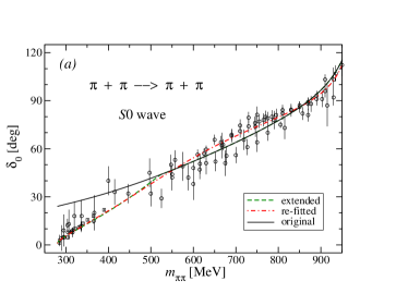
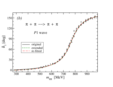
Figure 1: Phase shifts for the $S0$ wave ($a$) and $P1$ wave ($b$) amplitudes as a function of the effective two pion mass $m_{\pi\pi}$ for the original (solid line), extended (dashed line) and refitted (dash-dotted line) amplitudes considered in the text. Data are taken from Yura2010 .

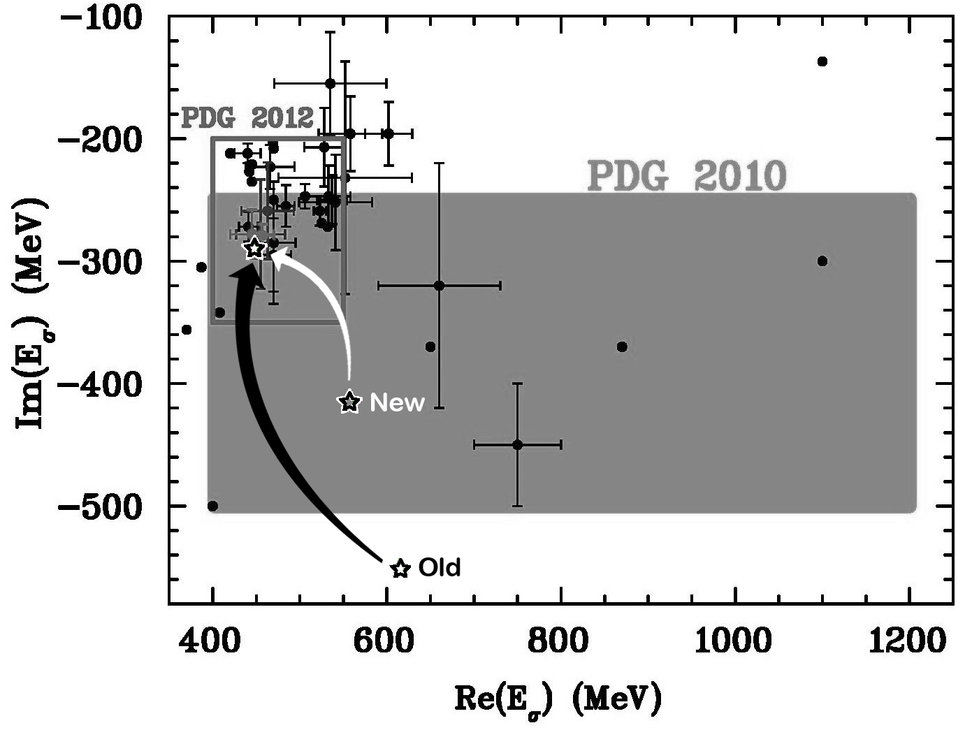
Figure 2: Shift of the $\sigma$ pole on sheet II after fitting to the GKPY equations. The stars in the lower part of figure denote the pole positions for the “Old” (original) and “New” amplitudes while the stars indicated by the arrows their positions after refitting. The big (PDG2010) and small (PDG2012) rectangles show area allowed by the Particle Data Tables in 2010 and 2012, respectively. Black points are positions of the poles listed in the Particle Data Tables published in 2010.

III Crossing symmetry constraints imposed on the amplitudes

In Ref. GKPY it has been presented that, due to only one subtraction, the GKPY equations are much more demanding, i.e. have significantly smaller uncertainties than the Roy equations with two subtractions. Therefore in this analysis we use only the GKPY equations which have the following general form

$${\mbox{Re }\bar{t}_{\ell}^{I}(s)} = \sum\limits_{I^{\prime}=0}^{2}C^{II^{\prime}}{t^{I^{\prime}}_{0}(4m_{\pi}^{2})}$$ (9)

$$+ \displaystyle\sum\limits_{I^{\prime}=0}^{2}\displaystyle\sum\limits_{\ell^{\prime}=0}^{3}\hskip 5.69046pt-\displaystyle\int\limits_{4m_{\pi}^{2}}^{\infty}\ ds^{\prime}K_{\ell\ell^{\prime}}^{II^{\prime}}(s,s^{\prime})\,{\mbox{Im }t_{\ell^{\prime}}^{I^{\prime}}(s^{\prime})},$$

where $t_{\ell^{\prime}}^{I^{\prime}}(s^{\prime})$ and $\bar{t}_{\ell}^{I}(s)$ are the input and output amplitudes, respectively, in a given partial wave $\ell,\ell^{\prime}$ with isospin $I,I^{\prime}$. The $C^{II^{\prime}}$ is the crossing matrix constant and $K_{\ell\ell^{\prime}}^{II^{\prime}}(s,s^{\prime})$ are kernels constructed for partial wave projected amplitudes with the imposed $s\leftrightarrow t$ crossing symmetry condition. Given $t^{I}_{\ell}(s)$ amplitude fulfills the crossing symmetry when real part of the output amplitude ${\mbox{Re }\bar{t}_{\ell}^{I}(s)}$ is equal to real part of the input one ${\mbox{Re }t_{\ell}^{I}(s)}$. In practice the part of Eq. (9) containing sums of the integrals is divided into two components. The first one contains contributions from lower energy parts (i.e. for $\sqrt{s}<1.42$ GeV) and is called “kernel part” while the second one includes contributions from amplitudes at higher energies and is called “driving terms”. Full expressions for the GKPY equations, together with derivation can be found in GKPY . The derivation starts with the Cauchy theorem applied to the full $\pi\pi$ amplitude depending on the $s$ and $t$ Mandelstam variables and composed of a set of partial waves afterwards integrated over $t$. Of course the Cauchy theorem can not be arbitrary used to a single partial wave without any physical constrain, which in this case is just the crossing symmetry relating all partial waves together.

In order to check how the $S0$ and $P1$ wave amplitudes described in Sec. II fulfill the crossing symmetry condition one has to use them as the input amplitudes in Eq. (9), i.e. integrate their imaginary parts with proper kernels from the threshold to 1.42 GeV. However, as we have already explained, both these amplitudes suffer from an improper description of the phase shifts near the $\pi\pi$ threshold region. Therefore, in order to allow the integration from the $\pi\pi$ threshold we have re-defined these amplitudes for energies $\sqrt{s_{1}}<\sqrt{s}<\sqrt{s_{0\ell}}$ where $\sqrt{s_{00}}$ and $\sqrt{s_{01}}$ are matching energies for the $S0$ and $P1$ waves, respectively. Above these energies the amplitudes remain fully equivalent to the “original” multichannel ones from Sec. II. Below these energies the amplitudes are parametrized as

$$\sin\,2\delta^{I}_{\ell} = \frac{4m_{\pi}k_{1}^{2\ell+1}}{\sqrt{s}}$$ (10)

$$\times \left[a^{I}_{\ell}+b^{I}_{\ell}k_{1}^{2}+c^{I}_{\ell}k_{1}^{4}+d^{I}_{\ell}k_{1}^{6}+\mathcal{O}(k_{1}^{8})\right],$$

where $\delta^{I}_{\ell}$ denotes the phase shift in the $\ell I$ wave. The parameters $a^{I}_{\ell}$ and $b^{I}_{\ell}$ are the scattering length and the so-called slope parameter, respectively, which can be fixed or fitted to the data and to the dispersion relations. In this analysis they were fixed at the values: $a^{0}_{0}=0.220$ $m_{\pi}^{-1}$, $a^{1}_{1}=0.0381$ $m_{\pi}^{-3}$, $b^{0}_{0}=0.278$ $m_{\pi}^{-3}$, and $b^{1}_{1}=0.00523$ $m_{\pi}^{-5}$ following the results of GKPY . The parameters $c^{I}_{\ell}$ and $d^{I}_{\ell}$ are used to match smoothly the phase shifts (10) with the multichannel “original” ones from Sect. II at the matching energies $\sqrt{s_{0\ell}}$. They are therefore calculated from the conditions that the phase shifts and their derivatives are continuous functions at $\sqrt{s_{0\ell}}$. Note that, one can also use other parametrizations in Eq. (10), e.g. the generalized effective range expansion or the form used in Ref. Bern .

Hereafter the $\pi\pi$-threshold-region corrected original amplitudes are denoted by “extended” amplitudes. In Fig. 1 the phase shifts of these amplitudes are presented as the dashed lines. Values of the matching energies $\sqrt{s_{00}}$ and $\sqrt{s_{01}}$ were fitted to the phase shifts to achieve the best description of the data. In Fig. 1, the values were found to be 525 and 643 MeV for the $S0$ and $P1$ amplitudes, respectively. Above these matching energies the original and extended amplitudes are equivalent and below they follow the expansions (10). One can see that the phase shifts of both extended amplitudes follow quite well the data below and above the matching energies.

Figure 3 illustrates that these extended amplitudes, however, do not fulfill the crossing symmetry condition especially for the $S0$ wave. A big difference is very well seen between the real parts of the input and output amplitudes, particularly below about 600 MeV. Also in the case of the $P1$ wave we see worse agreement between the input and the output amplitudes in comparison with that in Fig. 13 in GKPY where all partial waves have been fitted inter alia to the GKPY equations. The saddle point in the $S0$ output amplitude near the 500 MeV is caused by a noticeable change of curvature of the phase shifts seen in Fig. 1 near the matching energy.

Figure 3: Input (dashed line) and output (solid line) real parts of the $S0$ wave (upper figure) and $P1$ wave (lower figure) extended amplitudes, i.e. before fitting.

IV Results of refining

To improve agreement of the $S0$ and $P1$ wave amplitudes with the crossing symmetry, the corresponding extended amplitudes have been fitted to the GKPY dispersion relations (hereafter DR) and to the data. Taking advantage of the fact that these equations also apply to the $S2$ amplitude, the output of which strongly depends on the input amplitude $S0$, the $S2$ has also been fitted to the DR. The $S2$ input amplitude together with those for the $D0$, $D2$ and $F1$ has been taken from GKPY and fixed.

The total $\chi^{2}$ was composed of five parts

$$\chi^{2}=\sum_{l=1}^{2}\chi^{2}_{Data}(l)+\sum_{l=1}^{3}\chi^{2}_{DR}(l)$$ (11)

where $l=1,2,3$ itemizes the $S0$, $P1$ and $S2$ partial waves, respectively. Corresponding $\chi^{2}_{Data}(l)$ and $\chi^{2}_{DR}(\l)$ are expressed by

$$\chi^{2}_{Data}(l)=\sum_{i=1}^{N_{\delta}^{l}}\frac{(\delta_{i}^{exp}-\delta_{i}^{th})^{2}}{(\Delta\delta_{i}^{exp})^{2}}+\sum_{i=1}^{N_{\eta}^{l}}\frac{(\eta_{i}^{exp}-\eta_{i}^{th})^{2}}{(\Delta\eta_{i}^{exp})^{2}}$$ (12)

and

$$\chi^{2}_{DR}(l)=\sum_{i=1}^{N_{DR}}\frac{\left[{\rm Re}\>\bar{t}_{\ell}^{I}(s_{i})-{\rm Re}\>t_{\ell}^{I}(s_{i})\right]^{2}}{\left[\Delta{\rm Re}\>\bar{t}_{\ell}^{I}(s_{i})\right]^{2}}.$$ (13)

The experimental phase shifts $\delta_{i}^{exp}$ and inelasticities $\eta_{i}^{exp}$ for a given partial wave $\ell I$ (in all considered channels and with corresponding errors) are those used in Yura2010 for $m_{\pi\pi}$ above 0.6 GeV and 0.992 GeV, respectively. Apart from these data sets new data from ThrData for the near threshold region have been used. They have been obtained in experiments for $K_{l4}$ decays. Theoretical values of the phase shifts $\delta_{i}^{th}$ and inelasticities $\eta_{i}^{th}$ have been calculated from the multichannel amplitudes and from the threshold expansion (10) above and below the matching energy, respectively. The output amplitudes ${\rm Re}\,\bar{t}_{\ell}^{I}(s_{i})$ in (13) are calculated using the GKPY equations (9) and their errors are fixed to 0.01 in order to make the $\chi^{2}_{DR}=\sum\chi^{2}_{DR}(l)$ part of the total $\chi^{2}$ comparable with the $\sum\chi^{2}_{Data}(l)$. The input amplitudes ${\rm Re}\,t_{0}^{0}(s_{i})$ and ${\rm Re}\,t_{1}^{1}(s_{i})$ come directly from the extended amplitudes. The total number of the data points $N_{\delta}^{S0}+N_{\eta}^{S0}+N_{\delta}^{P1}+N_{\eta}^{P1}$ is 494 while $N_{DR}$ for DR was chosen to be 26 for each fitted partial wave to cover the $m_{\pi\pi}$ range from 0.31 GeV to 1.09 GeV with step 0.03 GeV.

In the fitting we changed only those parameters of the $S0$ and $P1$ extended amplitudes which can strongly influence the elastic region. The free parameters considered in the $S0$ wave are: the background parameters in the elastic channel $a_{11}$, $a_{1\sigma}$, $a_{1v}$, $a_{1\eta}$, $b_{1\sigma}$, $b_{1v}$ and $b_{1\eta}$, the matching energy $\sqrt{s_{00}}$ and poles of the resonances $f_{0}(500)$, $f_{0}(980)$ and $f_{0}(1500)$. The resonance $f_{0}(1500)$ was included because it was found to contribute significantly to the elastic phase shift below 1 GeV. Note that, in our previous analysis in Ref. FB20 this resonance was not included. In the $P$ wave only the background parameters $a$ and $b$, the matching energy $\sqrt{s_{01}}$ and the $\rho(770)$ were included. Total number of free parameters, i.e. those in the resonant and background parts in Eq. (2), is 31.

In Ref. Yura2010 the number and values of the fitted resonance parameters were restricted assuming a simple Breit–Wigner parametrization and some constraints imposed on positions of the poles. It ensured a compactness of resonance clusters and simultaneously reduces a number of free parameters: four for the $f_{0}(500)$, $f_{0}(980)$ and $\rho(770)$ and eight for the $f_{0}(1500)$. Following this assumption we refitted the considered free parameters of the $S0$ and $P1$ extended amplitudes. In Table 1 we show values of the full $\chi^{2}$ and its contributions from the $S0$ and $P1$ amplitudes and the DR before (extended) and after (refitted) fitting.

	$\chi^{2}$	$\chi^{2}_{Data}(S0)$	$\chi^{2}_{Data}(P1)$	$\chi^{2}_{DR}$
extended	1122.5	339.4	305.1	478.0
refitted	639.8	279.3	302.0	58.6

Table 1: Values of the $\chi^{2}$ for the extended (before fitting) and refitted (after fitting) amplitudes assuming constraints on resonance parameters.

Very big changes are seen in the $\chi^{2}_{Data}(S0)$ and $\chi^{2}_{DR}$ components. The big initial values are given mainly by the ill behavior of the extended amplitudes below $\approx$800 MeV which reflects their deficiency due to the crossing symmetry condition. This effect is also seen very well in Fig. 3 below about 600 MeV. The $\chi^{2}$ per number of degrees of freedom in this fit is $\chi^{2}/n.d.f.$ = 639.8/(494+78-31)=1.18.

Positions of the refitted poles changed notably for the $f_{0}(500)$, in particular those on sheets II and VII. The shift of the former was from $617-i\,554$ to $463-i\,296$ MeV which makes the new value well compatible with results based on ChPT and Roy-like equations Caprini:2005zr . Positions of poles of other resonances changed moderately by only few tens of per cent or less. The matching energy in the $S0$ wave became significantly smaller, $\sqrt{s_{00}}=394$ MeV, which points to an improvement of the low-energy behavior of the multichannel amplitude above $\sqrt{s_{00}}$. Small values of the fitted background parameters indicate a small importance of the background part of the $S$-matrix, which is consistent with the spirit of our approach to the multichannel analysis of data presented in Ref. Yura2014 . The only small disruption of the method stems from a negative value of the elastic background parameter, $a_{11}=-0.0644$, suggesting that some part of description is still missing. The absolute value of $a_{11}$ is, however, small and the result is therefore acceptable.

To improve the result we refitted the extended amplitudes again, removing now the constraints imposed in the clusters on resonance poles for the $f_{0}(500)$, $f_{0}(980)$, $f_{0}(1500)$ and $\rho(770)$. In this case the number of free parameters was larger (43) but improvement of the $\chi^{2}$ makes this fit a bit better: $\chi^{2}/n.d.f.$ = 605.5/(494+78-43)=1.14. Results of fitting with unconstrained resonance parameters are shown in Tables 2–6.

	$\chi^{2}$	$\chi^{2}_{Data}(S0)$	$\chi^{2}_{Data}(P1)$	$\chi^{2}_{DR}$
extended	1122.5	339.4	305.1	478.0
refitted	605.5	269.0	300.9	35.6

Table 2: Values of the $\chi^{2}$ for the extended (before fitting) and refitted (after fitting) amplitudes without the constraints on resonance parameters.

Table 2 shows the components of the total $\chi^{2}$ before and after fitting with unconstrained parameters of the resonances. An appreciable improvement with respect to the previous result is observed in the $\chi^{2}_{DR}$: $59\rightarrow 36$. This suggests that disabling the compactness of the resonance clusters allows the amplitudes to better conform the crossing symmetry condition driven by the GKPY equations.

Sheet		extended	refitted
	$f_{0}(500)$
II	$E_{r}$	$616.5$	$455.9$
	$\Gamma_{r}/2$	$554.0$	$295.4$
III	$E_{r}$	$621.8$	$826.4$
	$\Gamma_{r}/2$	$554.0$	$168.4$
VI	$E_{r}$	$598.3$	$709.4$
	$\Gamma_{r}/2$	$554.0$	$185.3$
VII	$E_{r}$	$593.0$	$243.2$
	$\Gamma_{r}/2$	$554.0$	$2093.9$
	$f_{0}(980)$
II	$E_{r}$	$1009.2$	$998.8$
	$\Gamma_{r}/2$	$31.3$	$\,\,\,23.4$
III	$E_{r}$	$985.8$	$965.9$
	$\Gamma_{r}/2$	$58.0$	$\,\,\,21.9$
	$f_{0}(1500)$
II	$E_{r}$	$1498.3$	$1441.7$
	$\Gamma_{r}/2$	$198.8$	$164.1$
III	$E_{r}$	$1502.4$	$1514.4$
	$\Gamma_{r}/2$	$236.8$	$97.12$
IV	$E_{r}$	$1498.3$	$1468.5$
	$\Gamma_{r}/2$	$193.0$	$145.5$
V	$E_{r}$	$1498.3$	$1435.3$
	$\Gamma_{r}/2$	$198.8$	$144.2$
VI	$E_{r}$	$1494.6$	$1507.0$
	$\Gamma_{r}/2$	$194.0$	$162.8$
VII	$E_{r}$	$1498.3$	$1493.3$
	$\Gamma_{r}/2$	$193.0$	$172.7$

Table 3: Positions of the poles in the $S0$ amplitude before (extended) and after (refitted) fitting with unconstrained resonance parameters. Real and imaginary parts of the poles are given by $\sqrt{s_{r}}=E_{r}-i\Gamma_{r}/2$ in MeV.

Sheet		extended	refitted
	$\rho(770)$
II	$E_{r}$	$766.4$	$765.1$
	$\Gamma_{r}/2$	$72.4$	$73.2$
III	$E_{r}$	$766.4$	$915.0$
	$\Gamma_{r}/2$	$72.4$	$23.3$
VI	$E_{r}$	$766.4$	$0.4$
	$\Gamma_{r}/2$	$72.4$	$2.1$
VII	$E_{r}$	$766.4$	$1059.2$
	$\Gamma_{r}/2$	$72.48$	$0.01$

Table 4: Positions of the poles in the $P1$ amplitude before and after fitting with unconstrained resonance parameters. Real and imaginary parts of the poles are given by $\sqrt{s_{r}}=E_{r}-i\Gamma_{r}/2$ in MeV.

Tables 3 and 4 show positions of the poles in the $S0$ and $P1$ amplitudes before and after fitting with unconstrained resonance parameters. Significant change of the pole positions is apparent for the $\sigma$ meson. The dominant pole on the sheet II, which produces the biggest part of the phase shifts below 1 GeV, was now shifted by $161+i\,259$ MeV towards the value recommended by PDG Tables 2012 PDGTables2012 . It is shown in Fig. 2 where the original pole of the multichannel amplitude Yura2010 is denoted by “Old”. Before fitting to the DR that pole was located even behind the range proposed by Particle Data Group before 2012 (denoted in the figure by “PDG2010”) PDGTables2010 . After fitting, the new value $455.9\pm 8-i\,295.4\pm 5$ MeV for the input amplitude and $449.3\pm 14-i\,288.7\pm 14$ MeV for the output one locate very close to the center of the new - much smaller range given by the PDG2012 PDGTables2012 and is in a good agreement, e.g. with the value $441^{+16}_{-8}-i\,272^{+9}_{-13}$ MeV from Caprini:2005zr . Large changes are observed also for the other pole positions, especially for the $\sigma$ meson. The quite small difference between $\sigma$ pole positions in the input and the output amplitudes is, as one can see in Fig. 4, due to a good agreement between them after fitting to the data and the DR. In the whole text and in the tables we present position of the poles only for the input amplitudes.

The parameters of background changed moderately as it is seen in Tables 5 and 6. Similarly as in the previous fit some of the parameters acquired negative values, e.g. $a_{11}$, $a_{1\sigma}$, $b_{1\eta}$ and $b$, disrupting a bit the philosophy of the multichannel approach in Ref. Yura2010 . However, as the absolute values are small this result is still acceptable. Value of the matching energy in the $S0$ wave is smaller than in the previous fit suggesting that in this case the multichannel amplitude above this energy is more flexible and can better accommodate requirements of the GKPY equations.

Parameter	value in the amplitude
	extended	refitted
$a_{11}$	0.0124	-0.0596
$a_{1\sigma}$	0.0	-0.1299
$a_{1v}$	0.1004	0.1965
$a_{1\eta}$	-0.0606	0.0099
$b_{1\sigma}$	0.0	0.0069
$b_{1v}$	0.0469	0.1011
$b_{1\eta}$	0.0	-0.0052
$\sqrt{s_{00}}$	525.7	382.2

Table 5: Values of the background parameters and the matching energy $\sqrt{s_{00}}$ (in MeV) for the $S0$ wave before and after fitting with unconstrained resonance parameters.

Parameter	value in the amplitude
	extended	refitted
$a$	-0.2851	-0.34459
$b$	0.00011	-0.00020
$\sqrt{s_{01}}$	643.6	635.4

Table 6: Values of the background parameters and the matching energy $\sqrt{s_{01}}$ (in MeV) for the $P1$ wave before and after fitting with unconstrained resonance parameters.

Figure 4 presents a comparison of the input and output refitted $S0$ and $P1$ amplitudes. Comparison with Fig. 3 shows how much the input and output amplitudes have changed. The difference between them has significantly diminished what allows us to conclude that now the $\pi\pi$ amplitudes fulfill the crossing symmetry really much better than before the fitting.

Figure 4: Input (dashed line) and output (solid line) real parts of the $S0$ (upper figure) and the $P1$ (lower figure) amplitudes after fitting.

It is desirable and instructive to check a stability of the results of analysis for the position of the $\sigma$ pole with respect to the definition of $\chi^{2}_{DR}$ in Eq. (13). To this end several additional fits with various errors and numbers of chosen points for the $\chi^{2}_{DR}$ have been performed. The errors were chosen 2, 3 and 4 times smaller or larger than 0.01 corresponding to presented in Table 1 results, and the number of points, $N_{DR}$, was the same (26) or two times bigger. The uncertainties of the real and imaginary parts of the $\sigma$ pole positions resulting from these changes proved to be much smaller than the error 14 MeV found in our best fit. They were: 3.4 MeV for the real part and 3.3 MeV for the imaginary one. Values of the $\chi^{2}$ for the experimental data used in the fits varied between 1.08 and 1.27 per degree of freedom. Clearly, variations of the $\chi^{2}_{DR}$ were larger but they followed changes in the error and the number of points.

Summarizing this check, one has to emphasize the clear stability of the results presented in the analysis and their significant independence from the chosen definition of $\chi^{2}$. Nevertheless in other similar analyses, particularly in those made with other experimental data leading to amplitudes deviating significantly from those allowed by the crossing symmetry condition (see for example Section VII in GKPY ), one has to always choose a definition of the $\chi^{2}_{DR}$ giving magnitudes of the same order as the $\chi^{2}_{Data}$.

As the most significant effect of refining the amplitudes was found to be the shift of the $\sigma$ pole, it is also desirable to show whether this effect depends on specific properties of the $S0$ amplitude or on the imposed crossing symmetry condition. For this purpose we have constructed a new version of the $S0$ input amplitude removing also imperfection of the old one which we found during our calculations, particularly a small violation of two-body unitarity around 1.2 GeV. Parameters of the new amplitude were not fitted to the DR but only to the same data and following the same method as in Ref. Yura2010 . The result of fitting is a bit worse than that in Yura2010 , $\chi^{2}$ = 302.3/(294-38)= 1.18 (1.11 in Ref. Yura2010 ), but the new amplitude is without the shortcoming due to unitarity. Moreover, in this new amplitude the $\sigma$ pole on sheet II at $562.9-i\,417.1$ MeV (denoted in Fig. 2 by “New”) is nearer to the PDG 2012 region than before. Especially the magnitude of imaginary part is smaller by 137 MeV. In Table 7 we show positions of all poles of the new $S0$ amplitude on the Riemann surface.

Table 7: The pole clusters for the new refitted $S0$ wave amplitude. $\!\sqrt{s_{r}}={\rm E}_{r}-i\Gamma_{r}/2\!$  in MeV is given.

Sheet		II	III	IV	V	VI	VII	VIII
$f_{0}(500)$	$\!{\rm E}_{r}\!$	$562.9\pm 4.9$	$594.7\pm 7.8$			$615.1\pm 39.6$	$583.3\pm 17.4$
	$\!\Gamma_{r}/2\!$	$417.1\pm 14.9$	$417.1\pm 14.9$			$417.1\pm 14.9$	$417.1\pm 14.9$
$f_{0}(980)$	$\!{\rm E}_{r}\!$	$1007.6\pm 3.0$	$984.5\pm 5.4$
	$\!\Gamma_{r}/2\!$	$29.4\pm 1.5$	$55.1\pm 3.4$
$f_{0}(1370)$	$\!{\rm E}_{r}\!$		$1397.0\pm 6.3$	$1397.0\pm 6.3$	$1277.0\pm 50.2$	$1277.0\pm 50.2$
	$\!\Gamma_{r}/2\!$		$216.5\pm 13.2$	$180.1\pm 11.1$	$180.1\pm 11.1$	$216.5\pm 13.2$
$f_{0}(1500)$	$\!{\rm E}_{r}\!$	$1496.6\pm 4.7$	$1502.7\pm 3.8$	$1496.6\pm 4.7$	$1496.6\pm 4.7$	$1502.1\pm 2.9$	$1496.6\pm 4.7$
	$\!\Gamma_{r}/2\!$	$203.5\pm 4.5$	$223.9\pm 5.2$	$198.7\pm 7.4$	$203.5\pm 4.5$	$187.9\pm 4.0$	$198.7\pm 7.4$
$f_{0}(1710)$	$\!{\rm E}_{r}\!$				$1736.0\pm 26.6$	$1736.0\pm 26.6$	$1736.0\pm 26.6$	$1736.0\pm 26.6$
	$\!\Gamma_{r}/2\!$				$108.3\pm 16.6$	$85.5\pm 11.8$	$43.3\pm 14.1$	$66.1\pm 13.8$

The new background parameters in Eq.(4) are: $a_{11}=-0.0131\pm 0.0019$, $a_{1\sigma}=0$, $a_{1v}=0.046\pm 0.011$, $a_{1\eta}=-0.0302\pm 0.0025$, $b_{11}=b_{1\sigma}=b_{1\eta}=0$, $b_{1v}=0.0573\pm 0.0071$, $a_{21}=-3.5456\pm 0.0188$, $a_{2\sigma}=0.6778\pm 0.0850$, $a_{2v}=-4.28\pm 0.44$, $a_{2\eta}=-0.1857\pm 0.0304$, $b_{21}=0$, $b_{2\sigma}=0.6499\pm 0.0886$, $b_{2v}=1.49\pm 1.74$, $b_{2\eta}=0.1011\pm 0.0265$, $b_{31}=0.3825\pm 0.0412$, $b_{3\sigma}=b_{3v}=b_{3\eta}=0$, $s_{\sigma}=1.638~{}{\rm GeV}^{2}$, $s_{v}=2.126~{}{\rm GeV}^{2}$. In the new extended $S0$ amplitude the matching energy is $\sqrt{s_{00}}=406.5$ MeV. Note that, similarly as in our previous fits starting with the “old” amplitude the parameter $a_{11}$ is negative.

We used this new extended $S0$ amplitude in the DR analysis keeping all other ingredients unchanged as in our previous two fits. During the fitting we let all poles of resonances to vary independently as we did it in our second fit with the old extended $S0$ amplitude. Values of $\chi^{2}$ are shown in Table 8.

	$\chi^{2}$	$\chi^{2}_{Data}(S0)$	$\chi^{2}_{Data}(P1)$	$\chi^{2}_{DR}$
extended	1085.4	302.3	305.1	478.0
refitted	607.8	274.2	293.9	39.7

Table 8: Values of the $\chi^{2}$ for the new extended (before fitting) and refitted (after fitting) amplitudes.

The fit is equally good as the previous one: $\chi^{2}/n.d.f.$ = 607.8/(494+78-43)=1.15. The $\sigma$ pole on sheet II is now at $459.0\pm 8-i\,292.3\pm 5$ MeV for the input amplitude and at $445.2\pm 14-i\,296.4\pm 14$ MeV for the output one which is very well consistent with the previous results (see Fig. 2). This suggests that the $\sigma$ pole position is prescribed rather by the GKPY equations than by the data or a structure of the $S0$ amplitude.

In order to know how released scattering length parameters, i.e., $a^{0}_{0}$ and $a^{1}_{1}$ affect the value of total $\chi^{2}$ for the $S0$ and $P1$ wave, we made them free and performed fit again. The total $\chi^{2}/n.d.f.$ slightly changed from 1.145 to 1.137 which is neglectable. Values of the fitted scattering lengths were: $a^{0}_{0}=0.224$ $m_{\pi}^{-1}$, $a^{1}_{1}=0.0340$ $m_{\pi}^{-3}$.

V Uniqueness of the results

Uniqueness of the results on the $\sigma$ pole position presented in the previous section can be proved using purely mathematical arguments. One should start, however, with the arguments for uniqueness of results obtained in the dispersive data analysis presented in Ref. GKPY ; PreciseDet . These have been received without any model assumptions about specific energy dependence of the $\pi\pi$ amplitudes. Another although similar analysis performed for the Roy equations has used two assumptions for values of the $S0$ wave amplitude at 800 MeV and at the $\pi\pi$ threshold A4 . In accordance with the method described in Ref. Wanders2000 due to these two boundary conditions the authors found the unique analytical solution of the Roy equations below 800 MeV. The position of the $\sigma$ pole obtained in GKPY ; PreciseDet differs by less then one standard deviation from that received in A4 what ensures in correctness and uniqueness of the results found in analyses GKPY and PreciseDet using the GKPY equations.

Uniqueness of the new position of the $\sigma$ pole and of its movement found in our analysis after fit to the DR can be easily proved using only two simple arguments: trigonometric relations satisfied by the $\pi\pi$ amplitudes and constraints given by the crossing symmetry condition. Looking at Fig. 5 with the $S0$ phase shifts corresponding to the extended and the refitted “Old” amplitudes one can observe significant differences between them especially from 500 to 800 MeV. One should also notice their completely different curvatures in this region caused by very different positions of the $\sigma$ pole presented in the previous Section.

Figure 5: Effective two-pion mass dependence of the phase shifts corresponding to the extended (dashed line) and refitted (solid line) “Old” amplitudes.

Real parts of the $S0$ input and output amplitudes presented in Fig. 3 correspond to the extended “Old” amplitude. In order to diminish difference between them one could intuitively think on a shifting down and up the real parts of the input amplitude below and above about 650 MeV respectively. The dependence of the real part of the amplitude on the phase shifts is presented in Fig. 6 and indicates that it would lead to decrease of the phase shifts in whole $m_{\pi\pi}$ region below about 900 MeV.

Figure 6: Dependence of the real and imaginary part of the amplitude on the phase shifts.

As is, however, seen on this figure it would reduce also the imaginary part of the amplitude. Comparison of the gradients of the imaginary and real parts of the amplitude in Fig. 7 (i.e., of the input and the output functions in Eq. (9), respectively) shows that for the phase shifts between around 22 and 112 degrees, i.e., within the range that we are interested in (see for example Fig. 1), just the imaginary part changes faster than the real one.

Figure 7: Gradient of the real and imaginary part of the amplitude as a function of the phase shifts.

Figure 8 presents energy dependence of the kernel part $KT^{00}_{00}$ being dominant in the full output amplitude ${\mbox{Re }\bar{t}_{0}^{0}(s)}$ in Eq. (9)

$$KT^{00}_{00}(s)=\hskip 1.42271pt-\displaystyle\int\limits_{4m_{\pi}^{2}}^{\Lambda}ds^{\prime}K_{00}^{00}(s,s^{\prime})\,{\mbox{Im }t_{0}^{0(IN)}}(s^{\prime})$$ (14)

where the parameter $\Lambda=(1.42\,\,\mbox{GeV})^{2}$ is upper limit of integration for the phenomenologically parametrized amplitudes (for details see Section II C of GKPY ).

Figure 8: Effective two pion mass dependence of the $KT^{00}_{00}$ term.

Characteristic and important feature is the positive value of the $KT^{00}_{00}$ below about 650 MeV and its negative value above this energy. Smooth and monotonic energy dependence of the input amplitude ${\mbox{Im }t_{0}^{0}}(s^{\prime})$ below about 800 MeV, caused by smooth behavior of the phase shifts, guarantees that such shape is produced by the kernel $K^{00}_{00}(s)$ in the Eqs. (9) and (14). This has been checked for different parametrizations of the phase shifts below 1 GeV.

Taking into account the bigger gradient of the ${\mbox{Im }t_{0}^{0}}(s^{\prime})$ than that of the ${\mbox{Re }t_{0}^{0}}(s^{\prime})$ and the shape of the $KT^{00}_{00}$, one can conclude that the intuitively expected and mentioned above decrease of the phase shifts would cause faster decrease of the output amplitude than decrease of the input one below around 650 MeV and faster increase above this energy. It means that the input amplitude could not catch up the escaping output one. Therefore in order to diminish distance between the real parts of the input and output amplitudes after fitting, the phase shifts must not decrease but increase below about 800 MeV. Then, finally, for some values of the increasing phase shifts, the input and output real parts can almost overlap what one can observe in Fig. 4 for the refitted amplitudes. Comparing the input and output real parts for the extended and refitted amplitudes in Figs. 3 and 4 one can easily check that below 650 MeV the input amplitude really increased and above this energy really decreased after fitting to the DR.

This pure mathematical analysis proofs that the increase of the phase shifts followed by change of the curvature after fitting, seen in Fig. 5, is natural and unique consequence of the trigonometry relations satisfied by the input and output amplitudes and of the energy dependence of the kernels given by the crossing symmetry condition. Analyzing the analytical structure of the amplitude in the complex energy plane one can conclude that such modification of the phase shifts can be produced only by the $\sigma$ pole on the IInd Riemann sheet moving toward the physical and the imaginary axis, i.e. by a narrower and lighter $\sigma$ meson. This we have illustrated in Fig. 2.

VI Conclusions

Very effective and simple way of modifying the amplitudes of the $\pi\pi$ interactions in the $S0$ and $P1$ waves has been presented. These modifications do not change mathematical structure of the original multichannel amplitudes (analytical properties on the Riemann surface) but only fit some of their parameters to the dispersion relations with the imposed crossing symmetry condition. After these modifications the amplitudes fulfill this symmetry from the $\pi\pi$ threshold to around 1.1 GeV and describe very well experimental data below about 1.8 GeV in all considered channels, e.g., $\pi\pi$, $K\bar{K}$, and $\eta\eta^{\prime}$. In the case of the amplitudes considered here, apart of finding new values of some of their parameters, the only important modification was introduction of the new part describing the near threshold region. The most important consequence of the fit to the dispersion relations was a significant movement of the $\sigma$ pole by several hundred MeV, i.e. by values comparable with its final mass and width. The new $\sigma$-pole position agrees very well with the value accepted in the Particle Data Tables in 2012 PDGTables2012 . The amplitudes, refitted using the presented method, can now be used as representative for the modeling of the $\pi\pi$ interactions what was impossible for the original ones with significantly too massive and too wide $\sigma$ meson. Another interesting result of refitting the multichannel amplitudes is a marked change of positions of the $f_{0}(1500)$ poles which are located well above the inelastic threshold. On the contrary imposing the crossing symmetry constraint practically did not affect the parameters of $\rho(770)$.

The method described here and presented example can be very helpful in refitting of other existing amplitudes which have similar problems as the original amplitudes analyzed here.

ACKNOWLEDGMENT The authors are grateful to Yu.S. Surovtsev for useful discussions. This work has been funded by the Polish National Science Center (NCN) Grant No. DEC-2013/09/B/ST2/04382 and was partially supported by the Grant Agency of the Czech Republic under Grant No. P203/12/2126.

References

- (1) R. García-Martín, R. Kamiński, J. R. Peláez, J. Ruiz de Elvira, and F.J. Ynduráin, Phys. Rev. D 83, 074004 (2011).
- (2) R. Kamiński, Phys. Rev. D 83, 076008 (2011).
- (3) R. García-Martín, R. Kamiński, J. R. Peláez, and J. Ruiz de Elvira, Phys. Rev. Lett. 107, 072001 (2011).
- (4) S. M. Roy, Phys. Lett. B 36, 353 (1971).
- (5) R. Kamiński, L. Leśniak, and B. Loiseau, Phys. Lett. B 551, 241 (2003).
- (6) M. R. Pennington, Ann. Phys. (N.Y.) 92, 164 (1975).
- (7) S. Descotes, N.H. Fuchs, L. Girlanda, and J. Stern, Eur. Phys. J. C 24, 469 (2002).
- (8) G. Colangelo, J. Gasser, and H. Leutwyler, Nucl. Phys. B 603, 125 (2001).
- (9) B. Ananthanarayan, G. Colangelo, J. Gasser, and H. Leutwyler, Phys. Rep. 353, 207 (2001).
- (10) I. Caprini, G. Colangelo, and H. Leutwyler, Phys. Rev. Lett. 96, 132001 (2006).
- (11) G. Wanders, Eur. Phys. J. C 17, 323 (2000).
- (12) K. Nakamura et al. (Particle Data Group), J. Phys. G 37, 075021 (2010).
- (13) J. Beringer et al. (Particle Data Group), Phys. Rev. D 86, 010001 (2012).
- (14) Yu. S. Surovtsev, P. Bydžovský, R. Kamiński, and M. Nagy, Phys. Rev. D 81, 016001 (2010).
- (15) Yu. S. Surovtsev, P. Bydžovský, and V.E. Lyubovitskij, Phys. Rev. D 85, 036002 (2012).
- (16) Yu. S. Surovtsev, P. Bydžovský, R. Kamiński, V.E. Lyubovitskij, and M. Nagy, Phys. Rev. D 86, 116002 (2012).
- (17) Yu. S. Surovtsev, P. Bydžovský, R. Kamiński, V.E. Lyubovitskij, and M. Nagy, Phys. Rev. D 89, 036010 (2014).
- (18) Yu. S. Surovtsev and P. Bydžovský, Nucl. Phys. A 807, 145 (2008).
- (19) I. Caprini, Phys. Rev. D 77, 114019 (2008).
- (20) J. R. Batley et al. (NA48/2 Collaboration), Eur. Phys. J. C 54, 411 (2008); S. Pislak et al. (BNL-E865 Collaboration), Phys. Rev. Lett. 87, 221801 (2001).
- (21) P. Bydžovský and R. Kamiński, Few-Body Syst. 54, 1149 (2013).