The Atacama Cosmology Telescope:
The LABOCA/ACT Survey of Clusters at All Redshifts

Abstract

We present a multi-wavelength analysis of eleven Sunyaev Zel’dovich effect (SZE)-selected galaxy clusters (ten with new data) from the Atacama Cosmology Telescope (ACT) southern survey. We have obtained new imaging from the Large APEX Bolometer Camera (345 GHz; LABOCA) on the Atacama Pathfinder EXperiment (APEX) telescope, the Australia Telescope Compact Array (2.1 GHz; ATCA), and the Spectral and Photometric Imaging Receiver (250, 350, and $500\,\rm\mu m$; SPIRE) on the Herschel Space Observatory . Spatially resolved $345\,\rm GHz$ SZE increments with integrated $\rm S/N>5$ are found in six clusters. We compute $2.1\,\rm GHz$ number counts as a function of cluster-centric radius and find significant enhancements in the counts of bright sources at projected radii $\theta<\theta_{2500c}$. By extrapolating in frequency, we predict that the combined signals from $2.1\,\rm GHz$-selected radio sources and $345\,\rm GHz$-selected SMGs contaminate the $148\,\rm GHz$ SZE decrement signal by $\sim 5\%$ and the $345\,\rm GHz$ SZE increment by $\sim 18\%$. After removing radio source and SMG emission from the SZE signals, we use ACT, LABOCA, and (in some cases) new Herschel SPIRE imaging to place constraints on the clusters’ peculiar velocities. The sample’s average peculiar velocity relative to the cosmic microwave background is $\left<v_{p}\right>=153\pm 383\,\rm km\,s^{-1}$.

1. Introduction

Galaxy clusters produce a spectral distortion in the cosmic microwave background (CMB) known as the Sunyaev Zel’dovich effect (SZE; Zel’dovich & Sunyaev, 1969; Sunyaev & Zel’dovich, 1970a). The thermal Sunyaev Zel’dovich effect (tSZ) signal is quantified by $Y_{\rm tSZ}\equiv\int y\,d\Omega$ in terms of the Compton parameter

$$y=\int\sigma_{T}\,n_{e}\frac{k_{\rm B}T_{e}}{m_{e}c^{2}}\,dl,$$ (1)

the Thomson cross section $\sigma_{T}$, Boltzmann’s constant $k_{\rm B}$, the electron density $n_{e}$, the electron temperature $T_{e}$, and the line-of-sight path length $dl$. The Compton parameter is insensitive to cluster redshift, allowing for the unbiased detection of massive clusters out to large distances. This selection is complementary to that of surveys using optical richness or X-ray flux, which generally yield lower-redshift cluster samples (for a review of the SZE in clusters, see e.g., Carlstrom et al., 2002). The mass function of SZE-selected galaxy clusters has been used to constrain the properties of dark energy, as well as the mean matter density $\Omega_{m}$ and amplitude of fluctuations $\sigma_{8}$ (e.g., Sehgal et al., 2011; Benson et al., 2013; Hasselfield et al., 2013b; Planck Collaboration et al., 2014b).

The number of known SZE-selected clusters is rising rapidly. The first surveys produced samples of $\sim 20$ blind SZE-detected clusters (Vanderlinde et al., 2010; Menanteau et al., 2010; Marriage et al., 2011). A sample of 68 SZE-selected clusters from the equatorial footprint of the Atacama Cosmology Telescope (ACT) survey has recently been presented by Menanteau et al. (2013) and Hasselfield et al. (2013b); 158 were detected in the first $720\,\rm deg^{2}$ of the South Pole Telescope (SPT) SZ survey (Reichardt et al., 2013); 677 were detected the full $2500\,\rm deg^{2}$ SPT-SZ survey (Bleem et al., 2014); and $\sim 1200$ more all-sky SZE cluster candidates have been catalogued by the Planck Collaboration et al. (2014c). Yet with samples ranging from nine (Sehgal et al., 2011) to eighteen (Vanderlinde et al., 2010; Benson et al., 2013) clusters, the first analyses found that the statistical errors on $w$ and $\sigma_{8}$ are already smaller than systematic errors due to uncertainties in the $Y_{\rm SZ}$-to-mass scaling relation. Hasselfield et al. (2013b) confirm this limitation by finding that the improvements in cosmological parameters from their sample of 68 SZE-selected clusters is mainly due to the inclusion of dynamical mass information, not to an increased sample size. Therefore, to further improve constraints from SZE-cluster cosmology using these larger samples, we need a better understanding of the scaling between integrated SZE signal and cluster mass in individual systems. For example, Sifón et al. (2013) have measured the dynamical masses of 16 massive SZE-selected clusters (nine of which are in our sample) and find that disturbed or merging systems could be biasing the derived $Y_{\rm SZ}$-to-mass scaling relations.

A number of physical processes are known to cause deviations from equilibrium scaling relations. Cluster mergers are predicted to cause departures from hydrostatic equilibrium, and can produce transient pressure enhancements that boost the SZE signal (e.g., Poole et al., 2006, 2007; Wik et al., 2008). Such pressure enhancements are invisible in X-ray observations of the massive cluster RXJ1347-1145, for example, but were revealed through high-resolution SZE-imaging to contribute $\sim 10\%$ of the bulk signal (Komatsu et al., 2001; Kitayama et al., 2004; Mason et al., 2010). Kinetic Sunyaev Zel’dovich (kSZ) signals due to clusters’ peculiar velocities can also introduce additional scatter to $Y_{\rm SZ}$ measurements. Hand et al. (2012) recently achieved a statistical detection of the pairwise kSZ signal from an ACT sample, but the peculiar velocity distribution of clusters remains unconstrained. Mroczkowski et al. (2012) found some evidence for large kSZ distortions in the triple merger system MACS J0717.5+3745, perhaps indicating that high-velocity substructures in merging clusters introduce additional deviations to $Y_{\rm SZ}$. Ruan et al. (2013) predict these deviations could bias $Y_{\rm SZ}$ results by $\sim 10\%$. The emission from bright galaxies near the clusters (in projection) can further bias the SZE signal. Synchrotron emission from star-forming galaxies and active galactic nuclei may “fill in” SZE decrements. Reese et al. (2012) estimate contamination from synchrotron sources to be $\lesssim 20\%$ in the $90\,\rm GHz$ SZE decrement based on high-resolution imaging of two ACT clusters, and Sayers et al. (2013) estimate that radio sources contaminate the $140\,\rm GHz$ SZE decrement by $\sim 1$-$20\%$. SZE increments, on the other hand, can be artificially enhanced by the strong infrared emission from dusty, high-redshift star-forming submillimeter galaxies (SMGs; for a review, see Blain et al., 2002). Gravitational lensing by the clusters’ potentials may increase contamination by lensed SMGs (e.g., Knudsen et al., 2008; Johansson et al., 2011; Jain & Lima, 2011) or introduce deficits in surface brightness at the location of the cluster (Zemcov et al., 2013), and disturbed or merging systems may be more susceptible to lensing effects due to their greater lensing efficiency (e.g., Meneghetti et al., 2007; Zitrin et al., 2013b). Benson et al. (2003) conclude that direct measurements of cluster peculiar velocities in maps with angular resolution $\gtrsim 1\,\rm arcmin$ will be limited by SMG contamination.

The number counts of the most massive clusters have the potential to constrain cosmological parameters. Unfortunately, these systems also tend to be most affected by the effects described above. Massive systems will produce the greatest gravitational lensing shear, and in our hierarchical universe, they are also commonly disrupted by recent merging activity. In this work, we aim to better understand how these considerations affect the observed SZE signals using high-resolution submillimeter and radio imaging of a representative sample of SZE-selected clusters.We present new observations at $345\,\rm GHz$ ($19.2^{\prime\prime}$ resolution) with the Large APEX Bolometer Camera (LABOCA; Siringo et al., 2009) on the Atacama Pathfinder EXperiment (APEX; Güsten et al., 2006) telescope and at $2.1\,\rm GHz$ ($5^{\prime\prime}$ resolution) with the Australia Telescope Compact Array (ATCA) of a sample of massive SZE-selected galaxy clusters. We call the project “LASCAR,” the LABOCA/ACT Survey of Clusters at All Redshifts, in honor of the Lascar volcano near the ACT site in northern Chile. We use these data to measure the properties of the clusters’ spatially resolved SZE increment signals, and quantify the degree of background and foreground radio and infrared galaxy contamination. Section 2 describes our cluster sample Section 3 presents observations and data reduction techniques. Section 4 assesses the SZE contamination by point sources. Section 5 uses the point-source subtracted multi-wavelength SZE maps to place constraints on cluster peculiar velocities. In Section 6 we discuss our results in the context of previous work, and in Section 7, we conclude. In our calculations, we assume a flat $\Lambda$CDM cosmology with $H_{0}=70\,\rm km\,s^{-1}\,Mpc^{-1}$, $\Omega_{M}=0.27$, and $\Omega_{\Lambda}=0.73$ (Komatsu et al., 2011).

2. Cluster sample

Our sample consists of eleven clusters with $148\,\rm GHz$ decrement signal-to-noise (S/N) $>4.7$ from the Atacama Cosmology Telescope (ACT; Fowler et al., 2007; Swetz et al., 2011) southern survey (Menanteau et al., 2010; Marriage et al., 2011). Our sample is selected from the 15 highest-S/N ACT southern clusters, and includes 9 of 10 clusters not known before ACT or SPT; it only excludes one cluster with $z<0.15$ and three clusters that had been previously mapped with AzTEC (D. Hughes, personal communication). The properties are listed in Table 1. The systems span a large redshift range, $z=0.3$–$1.1$, and have masses $M_{500c}\geq 3\times 10^{14}\,M_{\odot}$ (Menanteau et al., 2010; Sifón et al., 2013), where $M_{500c}=500\,(4\pi/3)\,\rho_{c}\,r_{500c}^{3}$, and $r_{500c}$ is the radius enclosing a mass density equal to $500\times$ the critical density of the Universe at the redshift of the cluster. We define the angular radius $\theta_{500c}=r_{500c}/D_{A}$, and use the typical scaling relation $M_{200c}\sim 1.6\,M_{500c}$ (Duffy et al., 2008) to convert from the dynamical masses of Sifón et al. (2013). Each SZE detection has been confirmed to be a rich optical cluster through followup imaging by Menanteau et al. (2010). Included in the sample are the notable cluster mergers ACT J0102-4915, also known as “El Gordo” (Menanteau et al., 2012), and 1E0657-56 (ACT J0658-5557), the original “Bullet” cluster (Markevitch et al., 2002).

3. Observations and data reduction

3.1. 345 GHz APEX/LABOCA

We obtained new LABOCA $345\,\rm GHz$ imaging of ten clusters in 2010–2011 (see Table 1). The LABOCA data for an eleventh cluster that is also detected by ACT (ACT-CL J0658$-$5557) are from the European Southern Observatory (ESO) archive. The following subsections describe the algorithms used to reduce the LABOCA data and extract SZE signals for our full sample of eleven clusters.

3.1.1 LABOCA observations

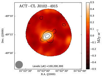
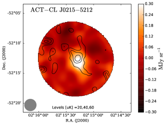
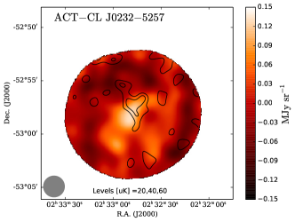
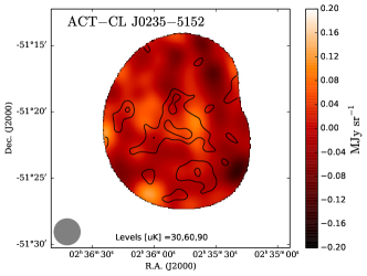
Figure 1.— LABOCA $345\,\rm GHz$ maps after iterative filtering, point-source subtraction, and smoothing. The color scale images represent $345\,\rm GHz$ surface brightness. The black contours represent the LABOCA-filtered ACT $148\,\rm GHz$ decrement intensities with levels indicated in the panels. The grey circle at the lower left represents the effective beam size of the LABOCA maps after smoothing to match the ACT resolution ($1.4^{\prime}$).

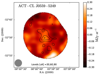
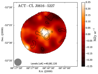
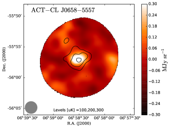
Figure 1.— Continued.

Observations were taken using the standard raster spiral mode, in which the telescope traces out one spiral every 35 seconds at each of four raster points defining a square with $27^{\prime\prime}$ sides. In polar coordinates $(r,\phi)$, the spiral track has an initial radius $r_{0}=18^{\prime\prime}$, a constant radial speed $\dot{r}=2.2^{\prime\prime}\,\rm s^{-1}$, and a constant angular rate $|\dot{\phi}|=\frac{\pi}{2}\,\rm rad\,s^{-1}$. The $345\,\rm GHz$ zenith opacity is interpolated between skydip measurements that punctuate observing sessions, and is used to correct for line-of-sight atmospheric absorption. Flux calibration is determined by observing a planet or secondary calibrator before each observing session, and the telescope pointing is monitored throughout the observations with periodic scans of bright quasi-stellar objects (QSOs). Scans that either had abnormally high RMS noise or were taken during rapidly changing atmospheric conditions were removed from the analysis. The total on-target integration time for the sample is 140 hr, as shown in Table 1.

The LABOCA main beam has a Gaussian profile with full width at half maximum (FWHM) of $19.2^{\prime\prime}$. The full beam${}^{\ref{laboca-cal}}$ includes broader, low-level wings and has total $\Omega=12.17\pm 0.43\,\rm nsr$. We use the full beam when computing integrated flux densities of extended sources, and we use the Gaussian main lobe when fitting PSF profiles to point sources.

3.1.2 LABOCA data reduction

We reduced the LABOCA data using the Python-based Bolometer Array Analysis Software (BoA) package. The data time-stream $T(c,t)$, a function of channel $c$ and time $t$, is first flux calibrated and corrected for atmospheric absorption. Next, median filtering at each time step is applied to all channels, then to each of twelve subgroups of channels that share readout cabling, then to each of four subgroups that share amplifier boxes. Despiking is performed between stages of median filtering, before a linear baseline is subtracted from each channel; channels with RMS noise greater than $4\times$ the median value are flagged. Low-frequency “$1/f$” noise is removed using BoA’s noise whitening algorithm flattenFreq, which sets the magnitudes of Fourier modes with frequencies less than some cutoff frequency $f<f_{c}$ to the average magnitude of those in the range $f_{c}<f<1.2\times f_{c}$. Because the celestial scanning velocity increases as a function of time during each scan as $v(t)\simeq(r_{0}+\dot{r}t)|\dot{\phi}|$, flattenFreq filters out emission on angular scales larger than the cutoff scale $s_{c}(t)$ given by

$$s_{c}(t) =v(t)/f_{c}=\left(28+3.5\times t\right)\,f_{c}^{-1}\;[\rm arcsec],$$ (2)

with $t$ in seconds and $f_{c}$ in Hz. The data are then gridded onto an equatorial $0.3^{\circ}\times 0.3^{\circ}$ image with $3.6^{\prime\prime}$ pixels (oversampling the beam by a factor of five in each direction). The resulting RMS sensitivities within $4^{\prime}$ of the centers of the beam-smoothed maps are presented in Table 1.

Table 1Cluster sample

	R.A.	Dec.		$\theta_{500c}$	$M_{500c}$		$t_{\rm obs}$	RMS
Name	(h:m:s)	($\circ:\prime:\prime\prime$)	$z$	($\prime$)	($10^{14}M_{\odot}$)	Project ID (P.I.)	(hr)	($\rm mJy\,bm^{-1})$
ACT-CL J0102$-$4915	01:02:53	-49:15:19	0.870	2.50	$10.2\pm 2.4$	M-087.F-0037-2011 (A. Baker)	11.3	2.4
ACT-CL J0215$-$5212	02:15:18	-52:12:30	0.480	3.16	$6.0\pm 1.7$	C-088.F-1772A-2011 (L. Infante)	17.6	2.0
ACT-CL J0232$-$5257	02:32:45	-52:57:08	0.556	2.42	$3.7\pm 1.4$	O-086.F-9302A-2010 (A. Baker)	17.0	1.7
ACT-CL J0235$-$5121	02:35:52	-51:21:16	0.278	5.18	$7.4\pm 2.1$	O-087.F-9300A-2011 (A. Baker)	12.2	2.1
ACT-CL J0245$-$5302	02:45:33	-53:02:04	0.300	3.08	$\simeq 3.1$	M-088.F-0003-2011 (A. Weiß)	11.6	2.0
ACT-CL J0330$-$5227	03:30:54	-52:28:04	0.442	4.08	$10.7\pm 2.5$	E-086.A-0972A-2010 (A. Baker)	8.1	1.9
ACT-CL J0438$-$5419	04:38:19	-54:19:05	0.421	4.53	$13.2\pm 3.1$	E-086.A-0972A-2010 (A. Baker)	18.3	1.6
ACT-CL J0546$-$5345	05:46:37	-53:45:32	1.066	1.75	$5.1\pm 2.6$	C-086.F-0668A-2011 (L. Infante)	16.3	1.6
ACT-CL J0559$-$5249	05:59:43	-52:49:13	0.609	3.08	$9.3\pm 2.7$	C-087.F-0012A-2011 (L. Infante)	13.3	2.8
ACT-CL J0616$-$5227	06:16:36	-52:28:04	0.684	2.60	$7.0\pm 3.1$	O-088.F-9300A-2011 (A. Baker)	14.8	2.1
ACT-CL J0658$-$5557	06:58:30	-55:57:04	0.296	3.44	$11.0\pm 6.8$	E-380-A-3036A-2007 (M. Birkinshaw)	16.5	2.2
						O-079.F-9304A-2007 (D. Johansson)

The above reduction steps, represented by $\mathcal{R}$, operate on time-stream data and return a gridded map, i.e., $I(\alpha,\delta)=\mathcal{R}[T(c,t),l]$, where the parameter $l$ represents the largest source size to which the entire scan remains responsive. The corresponding $f_{c}$ is found from Equation 2 by setting $s_{c}$ at $t=0$ (where it achieves its minimum value) equal to $l$ convolved with the LABOCA beam FWHM $\theta_{\rm beam}$:

$$f_{c}(l)=\frac{28}{\sqrt{l^{2}+\theta_{\rm beam}^{2}}}[\rm Hz],$$ (3)

for $l$ and $\theta_{\rm beam}$ in arcsec. For $l=0^{\prime\prime}$ and $l=120^{\prime\prime}$, $f_{c}(l)=1.47$ and $0.23\rm\,Hz$, respectively.

3.1.3 Iterative multi-scale algorithm

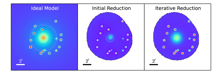
Figure 2.— Example of iterative reduction performance on an ideal cluster field. The cluster SZE signal is modelled using an iso-thermal beta profile with $\beta=0.86$ and core radius $r_{\rm c}=1^{\prime}$. SMGs are modeled as 15 point sources injected at random locations. The reduction adopts the observational parameters from ACT-CL J0546$-$5345. Left: Input $345\,\rm GHz$ noise-free model. Center: Output image after a single reduction (no iteration, Section 3.1.2). Right: Output image after running the iterative pipeline (described in Section 3.1.3). The white dotted dashed circle is centered on the modelled cluster with radius equal to the modeled core radius. White solid contours represent $345\,\rm GHz$ intensity levels of 1, 2, and $4\,\rm mJy\,beam^{-1}$. The fraction of recovered SZE signal within a $1.5^{\prime}$ aperture is initially $0.10$, increasing to $0.54$ after running the iterative multi-scale pipeline.

The filtering steps described above, primarily median filtering on cabling subgroups and noise whitening (Section 3.1.2), can remove the desired astrophysical emission from the data along with atmospheric noise. To recover this lost signal, we have developed an iterative, multi-scale pipeline. Our approach is inspired by techniques used by Enoch et al. (2006) and Nord et al. (2009). One important difference is that we maximize our sensitivity to low-level extended emission by using a series of matched filters to search for signal at multiple cluster-sized spatial scales, similar in nature to adaptive filtering algorithms (e.g., Scoville et al., 2007).

In the technique described below, a single “reduction” refers to one application of the standard pipeline described in Section 3.1.2. Our iterative pipeline is built “on top” of the standard pipeline by chaining together standard reductions using different values of $f_{c}$. The first step of the pipeline is reducing the data with aggressive filtering by setting the angular scale of fully preserved emission to $l=0^{\prime\prime}$. This first image, $I^{l=0^{\prime\prime}}_{1}$, is minimally affected by $1/f$ noise, although it has complete responsiveness only to point sources. High-significance structures in this first image are located by producing a S/N image $S(\alpha,\delta)$ using a spatial matched filter (e.g., Serjeant et al., 2003)

$$S=\frac{I\otimes k}{\sqrt{W\otimes k^{2}}},$$ (4)

where $k$ is a 2D Gaussian kernel with ${\rm FWHM}=\sqrt{l^{2}+\theta_{\rm beam}^{2}}$, and $W(\alpha,\delta)$ is a weight map defined by the inverse variance of time stream data within each pixel. Pixels where $S(\alpha,\delta)<S_{\rm thresh}$ are set to zero in $I^{l=0^{\prime\prime}}_{1}$. The significance level $S_{\rm thresh}$ is chosen so that we would expect $\leq 0.3$ spurious sources in the S/N map due to noise fluctuations (assuming a Gaussian noise distribution), and therefore depends on $l$ and the image size. This clipped image is then smoothed to the angular scale of interest by convolving with a normalized 2D Gaussian with ${\rm FWHM}=l$ to produce a model image $M^{l=0^{\prime\prime}}_{1}$. For the case of $l=0^{\prime\prime}$, a small amount of smoothing, $\rm FWHM=7^{\prime\prime}$, is still applied to help reduce sharp discontinuities in the model image. If the model image $M_{1}^{l=0^{\prime\prime}}$ is not empty, iteration proceeds and $M_{1}^{l=0^{\prime\prime}}$ is transformed into time stream data ${\mathcal{T}}[M_{1}^{l=0^{\prime\prime}}]$ and subtracted from the original time stream. This residual time stream $T-{\mathcal{T}}[M_{1}^{l=0^{\prime\prime}}]$ is then reduced using the procedure from Section 3.1.2, and the resulting residual image is added to $M_{1}^{l=0^{\prime\prime}}$ to produce the next image, $I_{2}={\mathcal{R}}[T-{\mathcal{T}}[M_{1}]]+M_{1}$. This process is carried out until the signal in the map converges, ($\Sigma(I_{n}-I_{n-1})\simeq 0$), and we are left with a final image $I_{N}$ and model $M_{N}$. Ten iterations are sufficient for the model image to converge.

Now we begin to search for larger spatial scale emission. $M_{N}^{l=0^{\prime\prime}}$ (the final, converged model image with $l=0^{\prime\prime}$ filtering) is subtracted from the original time streams, and the residual time stream is reduced with a relaxed filtering, initially, $l=30^{\prime\prime}$. If high-significance $30^{\prime\prime}$-scale emission is located using a matched filter, iteration begins again. This process is carried out for $l=0^{\prime\prime},30^{\prime\prime},60^{\prime\prime},$ and $120^{\prime\prime}$; the final image is the sum of all converged models, plus any residual low-level signal and the remaining noise:

$$I_{\rm final}=M_{f}+{\mathcal{R}}(T-{\mathcal{T}}[M_{f}]),$$ (5)

where $M_{f}$ is the sum of all scales’ converged model images $M_{f}=\Sigma_{l}{M_{N}^{l}}$. The array loses sensitivity quickly for angular scales that are larger than the typical size of contiguous subsets of channels that share cabling (i.e., $\gtrsim 6.7^{\prime}$); therefore, the pipeline is limited to $l\leq 120^{\prime\prime}$, which allows for recovery of emission on scales up to $\left<s_{c}(t,l=120^{\prime\prime})\right>\leq 6.5^{\prime}$.

Table 2SZE properties

	$T_{e}$	$\theta^{\prime}$		$v_{p}$	$S^{\rm SZE}_{\rm 345}(<\theta^{\prime})$	$Y^{\prime}_{\rm SZ}$
Name	$(\rm keV)$	$(\rm arcmin)$	SPIRE?	$(\rm km\,s^{-1})$	(mJy)	($10^{-10}\,\rm sr$)	S/N
$\rm S/N\geq 5$
ACT-CL J0102$-$4915	$14.5\pm 1.0$	2.2	✓	$-1100_{-2200}^{+1300}$ ($-2800_{-3100}^{+1700}$)	$276\pm 28$	$1.8_{-0.3}^{+0.3}$ ($1.4_{-0.3}^{+0.2}$)	9.7
ACT-CL J0215$-$5212	$5.9\pm 1.3$	1.9		$-1100_{-600}^{+400}$	$171\pm 21$	$0.8_{-0.1}^{+0.1}$	8.2
ACT-CL J0438$-$5419	$11.9\pm 1.2$	1.9	✓	$900_{-1000}^{+1000}$ ($600_{-1200}^{+1000}$)	$127\pm 15$	$0.9_{-0.1}^{+0.1}$ ($0.8_{-0.1}^{+0.1}$)	8.7
ACT-CL J0546$-$5345	$8.54^{+1.38}_{-1.05}$	1.9	✓	$-300_{-700}^{+700}$ ($-300_{-700}^{+700}$)	$162\pm 20$	$1.0_{-0.1}^{+0.1}$ ($0.9_{-0.1}^{+0.1}$)	8.2
ACT-CL J0616$-$5227	$6.6\pm 0.8$	1.9		$-300_{-600}^{+600}$	$160\pm 21$	$0.9_{-0.1}^{+0.1}$	7.7
ACT-CL J0658$-$5557	$10.8\pm 0.9$	1.6		$2500_{-1000}^{+1000}$	$121\pm 22$	$1.1_{-0.2}^{+0.1}$	5.4
$\rm S/N<5$
ACT-CL J0232$-$5257	$9.1\pm 2.1$	1.8		$-1200_{-1900}^{+1200}$	$67\pm 16$	$0.4_{-0.1}^{+0.1}$	4.3
ACT-CL J0235$-$5121	5.0	1.7	✓	$-1500_{-2800}^{+1800}$ ($-1500_{-2800}^{+1800}$)	$36\pm 16$	$0.2_{-0.1}^{+0.1}$ ($0.2_{-0.0}^{+0.1}$)	2.2
ACT-CL J0245$-$5302	5.0	1.9	✓	$500_{-600}^{+1200}$ ($500_{-600}^{+1200}$)	$53\pm 18$	$0.4_{-0.1}^{+0.1}$ ($0.4_{-0.1}^{+0.1}$)	2.9
ACT-CL J0330$-$5227	$4.32^{+0.21}_{-0.19}$	1.9	✓	$100_{-1000}^{+1000}$ ($100_{-800}^{+1000}$)	$70\pm 34$	$0.5_{-0.2}^{+0.2}$ ($0.5_{-0.2}^{+0.1}$)	2.1
ACT-CL J0559$-$5249	$8.09\pm 0.75$	1.5		$3100_{-1000}^{+1900}$	$41\pm 23$	$0.4_{-0.1}^{+0.1}$	1.8

We detect bright SMGs in all clusters and strong SZE increment signals (S/N$>3.5$) in six clusters (see Table 2). The final, converged, iteratively reduced $345\,\rm GHz$ images of all eleven clusters after point-source subtraction and smoothing are shown in Figure 1.

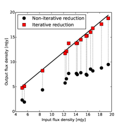
Figure 3.— Point source transfer function efficiency of the iterative LABOCA reduction pipeline. The circles and squares represent the input and output flux densities of 15 ideal LABOCA point sources with flux densities between 5–$19\,\rm mJy$ (see Figure 2) for a single run of the reduction pipeline (black circles), and for a full iterative reduction (red squares). The black line shows the relation $\rm output=input$. The average flux recovery fractions for single and iterative reductions are $0.50$ and $0.97$, respectively.

As an instructive check of our approach to data processing, we can compare our map of ACT J0658-5557 to the 345 GHz map made by Johansson et al. (2010) from the same LABOCA data using different reduction software (CRUSH), and to the $1^{\prime}$ resolution 150 GHz map of the cluster made with the APEX-SZ instrument. Johansson et al. (2010) deliberately filter the LABOCA data to suppress extended structure, including SZE increment signal. However, the flux densities they measure for the three most significantly detected SMGs in their Gaussian-matched-filtered map ($48.6\pm 1.3$, $15.1\pm 1.0$, and $6.9\pm 0.9\,{\rm mJy}$) agree well with those we have extracted from our own version of the map ($48\pm 2$, $13\pm 2$, and $7\pm 2\,{\rm mJy}$: Aguirre et al., in preparation). Halverson et al. (2009) fit an isothermal elliptical $\beta$ model to their SZE decrement observations and determine a projected core radius of $142\pm 18\,{\rm arcsec}$ that is well-matched to the size of the (rather asymmetric) structure we see in our 345 GHz map. Broadly speaking, our mapping algorithm produces results that are consistent with previous work that focuses on either point sources or extended emission.

3.1.4 Systematic uncertainties of iterative pipeline

In Figure 2, we show the results when a noise-free image of an ideal cluster model is transformed to time stream data and passed through the full iterative pipeline. We use an isothermal beta profile with $\beta=0.86$ and core radius $r_{r\rm c}=1^{\prime}$, typical parameters for SZE clusters in Marriage et al. (2011). Foreground and background SMGs are modeled by injecting 15 point sources with flux densities ranging between 5 and $20\,\rm mJy$ at random locations in the map. We define the transfer function efficiency (TFE) as the ratio of flux densities of structures in the final map divided by their “true” flux densities in the input model image. Point-source flux densities are measured using a least-squares fit to a circular Gaussian profile with a floating constant offset, and integrated SZE signal is measured as the integrated flux density within a circular aperture of radius $1.5^{\prime}$ (the typical radius used to extract SZE photometry in Section 5) after subtraction of point sources. For a single-pass reduction, the TFEs of point sources and the extended SZE signal are $0.50$ and $0.10$, and increase to $0.97$ and $0.54$ after running the full iterative pipeline. The spatially extended SZE signal is not fully recovered because of the pipeline’s inability to faithfully recover signals on scales larger than $120^{\prime\prime}$. Figure 2 displays the initial model, a single (non-iterative) reduction, and the final iterated image for our simulated cluster, and Figure 3 displays the input and output flux densities of individual point sources before and after iteration.

For extended SZE signals, the transfer function efficiency will range between $0.10$ and $0.54$ depending on whether the SZE signal was strong enough to trigger the iterative filter. The transfer function efficiency for extended emission is ignored in the following sections because identical filtering and aperture photometry is used in all SZE wavebands, and we only require relative photometry to derive peculiar velocities. For SMGs, the flux that remains lost after iteration is much lower than the typical statistical uncertainty of our measurements and can be ignored.

3.2. 148 GHz and 218 GHz ACT

We use the ACT 148 and $218\,\rm GHz$ maps, with beam FWHMs of $1.4^{\prime}$ and $1.1^{\prime}$ (Hasselfield et al., 2013a), respectively, to constrain the low frequency portions of the clusters’ SZE spectra. Before extracting the integrated flux densities $S_{148}$ and $S_{218}$ for each cluster, we filter the raw ACT maps to mimic the transfer function of our LABOCA observations, which attenuates emission from spatial scales larger than $\gtrsim 120^{\prime\prime}$. This filtering is done by first taking the 2D Fourier transform of $1\,\rm deg^{2}$ cutouts around the clusters in the ACT maps. We then apply the same frequency-domain filtering in 2D space for the ACT maps that the BoA algorithm flattenFreq performed on the 1D LABOCA time streams. To transform between temporal and spatial frequencies, we use the angular scanning speed of the LABOCA observations. We approximate the full continuous 35 second APEX raster spiral as a collection of circular scans at many different radii. One Fourier-filtered map is produced for each discrete scanning speed, and the final filtered maps used to extract $148\,\rm GHz$ and $218\,\rm GHz$ flux densities are taken to be the average of all individual velocity samplings. Beam solid angles at 148 and $218\,\rm GHz$ are taken from Hasselfield et al. (2013a).

We have tested our Fourier-based replication of the LABOCA pipeline spatial filtering by applying this Fourier filtering to the ideal cluster model from Section 3.1.4. We find that the fractional SZE signal recovered within a $1.5^{\prime}$ aperture ($\rm TFE\simeq$$0.53$) agrees with the result from the real iterative pipeline ($\rm TFE\simeq$$0.54$).

3.3. 2.1 GHz ATCA

3.3.1 ATCA Observations

We acquired $2.1\,\rm GHz$ Australia Telescope Compact Array (ATCA) observations of the ten clusters in our sample with new LABOCA observations. We used the $16\,\rm cm$-band receiver with the Compact Array Broadband Backend (CABB) giving 2049 $1\,\rm MHz$-wide channels spanning $1.1$–$3.1\,\rm GHz$. Observations were made in January 2011 (PI: Baker), December 2011 (PI: Baker), and April 2012 (PI: Lindner). All clusters have been observed with the 6A antenna configuration (baseline range $B=$628–$5939\,\rm m$), and ACT J0102-4915 has additional data in the 1.5B configuration ($B=$31–$4301\,\rm m$). For flux and bandpass calibration we used PKS 1934-638 (Reynolds, 1994). The Australia Telescope National Facility (ATNF) on-line calibrator database was used to choose one or more suitably bright, nearby, and compact phase calibrators for each cluster; these are listed in Table 3.

Table 3ATCA $2.1\,\rm GHz$ observations

			$t_{\rm obs}$
Month	Target	Phase cal	(hr)	Configuration
Jan 2011	ACT-CL J0232$-$5257	J0214-522	19.8	6A
	ACT-CL J0546$-$5345	J0539-530	21.0	6A
Dec 2011	ACT-CL J0102$-$4915	J0047-579	12.1	6A
	ACT-CL J0215$-$5212	J0214-522	8.6	6A
	ACT-CL J0235$-$5121	J0214-522	8.5	6A
	ACT-CL J0245$-$5302	J0214-522	10.3	6A
	ACT-CL J0330$-$5227	J0334-546	8.8	6A
	ACT-CL J0438$-$5419	J0522-611	8.1	6A
	ACT-CL J0559$-$5249	J0539-530	8.9	6A
	ACT-CL J0616$-$5227	J0539-530	7.8	6A
		J0522-611		6A
		J0647-475		6A
Apr 2012	ACT-CL J0102$-$4915	J0047-579	6.8	1.5B

The software package MIRIAD (Sault et al., 1995) was used to calibrate, flag, invert, and clean the visibility data. Radio frequency interference (RFI) that affected all channels at a given time or at all times for a certain channel was removed manually using pgflag and blflag. Transient RFI was removed using the automated flagging algorithm mirflag (Middelberg, 2006). Baseline 1–2 in the April 2012 data contained powerful broad-spectrum RFI and was entirely flagged. First-order multi-frequency synthesis images with robust parameter robust$=0$ were made using invert and mfclean. Two rounds of self-calibration were then carried out, one solving for phase only, and one for both phase and amplitude together. The final RMS sensitivities at phase center vary over the range 6.9–$12\,\rm\mu Jy\,beam^{-1}$ (see Table 4).

Table 4ATCA map properties

	$\left<\nu\right>$	$\theta_{\rm major}$	$\theta_{\rm minor}$	P.A.	map RMS
Target	(GHz)	($\prime\prime$)	($\prime\prime$)	($\circ$)	($\mu\rm Jy\,beam^{-1}$)
ACT-CL J0102$-$4915	2.15	6.13	3.09	-1.9	7.5
ACT-CL J0215$-$5212	2.16	4.66	2.93	-21.0	11.0
ACT-CL J0232$-$5257	2.13	4.80	3.06	6.0	8.1
ACT-CL J0235$-$5121	2.17	5.26	2.71	-10.0	10.9
ACT-CL J0245$-$5302	2.16	4.44	2.97	4.3	10.5
ACT-CL J0330$-$5227	2.17	5.06	2.73	17.7	11.7
ACT-CL J0438$-$5419	2.15	5.30	2.80	-19.6	11.9
ACT-CL J0546$-$5345	2.13	4.66	3.21	-3.1	6.9
ACT-CL J0559$-$5249	2.15	5.35	2.86	-13.1	9.6
ACT-CL J0616$-$5227	2.15	4.99	2.98	26.2	12.0

3.4. $Herschel\;observations$

To help constrain the high-frequency end of the SZE spectrum when deriving cluster peculiar velocities (see Section 5 below), we use newly obtained 250, 350, and $500\,{\rm\mu m}$ imaging of six targets in our sample using the Spectral and Photometric Receiver (SPIRE; Griffin et al., 2010) instrument on board the Herschel Space Observatory (Pilbratt et al., 2010). The six targets were prioritized within our ATCA sample of ten on evidence of having high mass (SZE decrement strength, optical richness, etc. from Menanteau et al. (2010) and Sifón et al. (2013)), although in the end they did not overlap perfectly with the five objects for which we detected strong SZE increments with LABOCA. All SPIRE observations used the Large Map mode with nominal map speed. For five of the six clusters observed (ACT-CL J0102-4915, ACT-CL J0235-5121, ACT-CL J0245-5302, ACT-CL J0438-5419, and ACT-CL J0546-5345), four repetitions apiece of $8^{\prime}\times 8^{\prime}$ maps centered at four different dither positions yielded a total of $4\times 4\times 139\,\rm s=2224\,{\rm s}$ of time on-source. For ACT-CL J0330-5227, we were able to fit in four repetitions of a $6^{\prime}\times 6^{\prime}$ map at a single position, for a total of $1\times 4\times 123\,\rm s=492\,{\rm s}$ on-source, and, consequently, a much shallower depth. All data were reduced using the Herschel Interactive Processing Environment (HIPE, version 10.3.0; Ott, 2010) using standard scripts. The final maps have angular resolutions 17.6, 23.9, and $35.0^{\prime\prime}$ with mean confusion-limited RMS map sensitivities of 7.4, 7.2, $7.2\,{\rm mJy\,beam^{-1}}$ in the 250, 350, and $500\,{\rm\mu m}$ bands, respectively, for all but ACT-CL J0330-5227.

The typical increment intensities relative to those at 345 GHz are expected to be approximately 0.05%, 2%, and 34% in observations at 250, 350, and $500\,{\rm\mu m}$, respectively. The high sensitivity and comparatively low angular resolution of Herschel/SPIRE, however, mean that our images all suffer badly from confusion: their brightness fluctuations are primarily due to the blending together of bright, unresolved sources (here, SMGs). Section 3.6 describes the approach we have used to disentangle SZE increment signal from this confused background.

3.5. Foreground Galactic dust subtraction

The SPIRE maps of ACT-CL J0245-5302 and ACT-CL J0546-5345 contain detectable diffuse emission from Galactic dust on large spatial scales. The mean dust temperatures within $10^{\prime}$ radii (covering the full extent of the SPIRE maps) of the cluster centers as measured by Planck are $T^{0245}_{D}=19.9\pm 0.7\,\rm K$ and $T^{0546}_{D}=20.1\pm 0.3\,\rm K$ (Planck Collaboration et al., 2014a). To remove the foreground dust emission from the maps, we first generate a model of the smoothly varying foreground dust signal by applying a median filter with kernel size $4^{\prime}$ to the $250\,\rm\mu m$ maps. This dust model image is then jointly fit to similarly filtered versions of the 350 and $500\,\rm\mu m$ maps using a modified blackbody thermal spectrum with emissivity fixed at $\beta=1.57$, the value measured in the directions of both clusters by Planck Collaboration et al. (2014a). The $250\,\rm\mu m$ dust model is then scaled according to the best-fit dust temperature and subtracted from the $350\,\rm\mu m$ and $500\,\rm\mu m$ maps.

We find best-fitting dust temperatures of $T^{0245}_{D}=23_{-1}^{+2}\,\rm K$ and $T^{0546}_{D}=19_{-1}^{+1}\,\rm K$. The reasonable consistency of our temperatures with the Planck results supports our assumption that Galactic dust is the cause of the observed diffuse signals.

3.6. The Sunyaev Zel’dovich effect

The deflection in CMB intensity due to the thermal SZE for a single-temperature gas is (Zel’dovich & Sunyaev, 1969; Sunyaev & Zel’dovich, 1970b)

$$\Delta I_{\rm tSZ}=y\,I_{0}\,g(x,T_{e}),$$ (6)

in terms of the scaled frequency $x\equiv h\nu/k_{\rm B}T_{\rm CMB}$, $I_{0}=2(k_{\rm B}T_{\rm CMB})^{3}/(hc)^{2}=22.87\,\rm Jy\,arcmin^{-2}$, the electron temperature $T_{e}$, and the Compton parameter $y$ (see Equation 1). The function $g\left(x,T_{e}\right)$ is the derivative of the Planck function ($dB_{\nu}/dT$) multiplied by the SZE spectrum,

$$g(x,T_{e})=\frac{x^{4}e^{x}}{\left(e^{x}-1\right)^{2}}\left(x\frac{e^{x}+1}{e^{x}-1}-4\right)\left[1+\delta_{\rm tSZ}\left(x,T_{e}\right)\right],$$ (7)

where $\delta_{\rm tSZ}$ represents relativistic corrections that become important at high electron temperatures, especially when $x\gg 1$.

The change in CMB intensity due to the kSZ effect is given by (Sunyaev & Zel’dovich, 1972)

$$\Delta I_{\rm kSZ} =-\tau_{e}\,I_{0}\,\left(\frac{v_{p}}{c}\right)\frac{dB_{\nu}}{dT}$$

$$=-\tau_{e}\,I_{0}\,\left(\frac{v_{p}}{c}\right)\frac{x^{4}e^{x}}{\left(e^{x}-1\right)^{2}}\left[1+\delta_{\rm kSZ}\left(x,T_{e}\right)\right],$$ (8)

where $v_{p}$ is the cluster line-of-sight peculiar velocity with respect to the CMB in the cluster rest frame, the optical depth to electron scattering $\tau_{e}=\int\sigma_{\rm T}\,n_{e}\,dl$, and $\delta_{\rm kSZ}$ represents higher-order relativistic corrections.

Equations 6 and 3.6 are shown to highlight the leading order terms in the thermal and kinetic SZE signal. In our analysis, we do not use the analytic expressions, but instead compute the SZE signal with numerical integration using the C++ package SZPACK (Chluba et al., 2012, 2013). SZpack allows for quick computations of the relativistic tSZ and kSZ signals with $10^{-5}$ precision for temperatures up to $T_{e}\simeq 25\,\rm keV$ at frequencies up to and including the high-frequency Herschel SPIRE bands ($x\lesssim 20$) and peculiar velocities up to $|v_{\rm pec}|/c\simeq 0.1$ ($|v_{\rm pec}|\simeq 30\times 10^{3}\,\rm km\,s^{-1}$).

3.7. Isolating SZE signal in SPIRE maps

We isolate the SZE signal in the $350\,\rm\mu m$ and $500\,\rm\mu m$ SPIRE maps by using the $250\rm\,\mu m$ map (which contains a negligible contribution from SZE signals compared to the 350 and $500\,\rm\mu m$ bands) to derive a model for the confused SMG background. This approach was presented by Zemcov et al. (2010), but our implementation of it differs in several important respects. For a given cluster, we begin by producing a model of the background SMG confusion signal at $250\,\rm\mu m$ ($\mathcal{B}_{250}$) by applying a median filter with kernel size $\rm 3\times\,FWHM_{250}$ to the $250\rm\,\mu m$ image. We then smooth $\mathcal{B}_{250}$ to the angular resolution of the $350\,\rm\mu m$ image to produce an estimate of the confused background at $350\,\rm\mu m$, $\mathcal{B}_{350}$.

We next locate bright sources that stand out from the confused $250\rm\,\mu m$ background by first subtracting $\mathcal{B}_{250}$ from the original $250\rm\,\mu m$ image, and then searching for point sources in the resulting background-subtracted image using a spatial matched filter (e.g., Serjeant et al., 2003). The matched filter identifies high S/N peaks, which are then individually fit to an ideal $250\,\rm\mu m$ PSF with positions and flux densities allowed to vary. Sources are extracted to a S/N level of $4.5\sigma$; we find 100–200 sources per cluster. The properties of the $250\,\rm\mu m$ point sources represent a starting point for modelling bright SMGs at $350\,\rm\mu m$.

The $350\,\rm\mu m$ map is then fit to a $3N+2$-parameter model consisting of the confused background plus bright SMGs. The offset $a$ and scaling $b$ of the confused background template and the remaining $3N$ parameters representing the coordinates $\vec{x}^{\prime}$ and flux densities ($S$) of bright SMGs are combined into a parameter vector $\theta=(\{\vec{x}^{\prime}_{i},S_{i}\}_{n=1}^{N},a,b)$. The resulting model

$${\mathcal{M}}(\vec{x};\theta)=a+b\,{\mathcal{B}_{350}+\sum_{n}^{N}S_{n}\,e^{-\left|\vec{x}-\vec{x}^{\prime}_{n}\right|^{2}/2\sigma_{n}^{2}}},$$ (9)

is then fit to the $350\,\rm\mu m$ image using least-squares minimization. The optimization is carried out using Powell’s method (Powell, 1964), where in each iteration the parameters are minimized individually. Powell’s method works well for this problem because each source affects only a small fraction of the data. This joint optimization naturally accommodates the increased blending that occurs in the longer wavelength images. A $350\,\rm\mu m$ source is considered an SMG and subtracted from the map if its final converged position is less than a distance $0.25\,\rm FWHM_{350}$ from the location for that source intially guessed from the $250\,\rm\mu$ data. To avoid fitting the confusion model to the cluster signal itself, the above optimization is carried out once while masking in central cluster region and allowing all parameters in $\theta$ to vary, then once more without the mask and holding $a$ and $b$ fixed at their previously fit values.

The process described above is repeated (independently, but in the same way) for the SPIRE $500\,\rm\mu m$ map. Emission that remains in the $350\,\rm\mu m$ and $500\,\rm\mu m$ maps after subtraction of the $250\,\rm\mu m$-inspired SMG background model is due either to (a) SZE increment, or (b) SMGs that were not detected in the $250\,\rm\mu m$ map at all, possibly because they lie at very high redshifts. After removing the SMG confusion noise, the 350 and $500\,{\rm\mu m}$ maps have mean RMS sensitivities of 2.9 and $2.7\,{\rm mJy\,beam^{-1}}$, respectively.

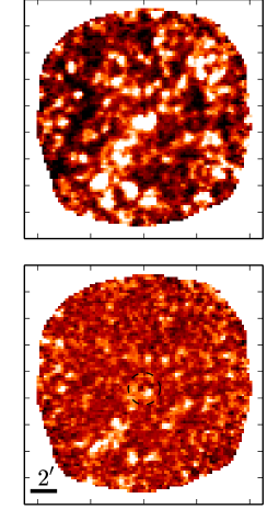
Figure 4.— Confusion signal removal process for cluster ACT–CL J0102-4915. The upper panel shows the original SPIRE $500\,\rm\mu m$ image with confusion-dominated RMS noise of $6.8\,\rm mJy\,beam^{-1}$. The color scale ranges linearly between -10 and $10\,\rm mJy\,beam^{-1}$. The lower panel shows the same map after running the SZE-extraction from Section 3.7 to remove the confused SMG background; here the RMS noise is reduced to $2.2\,\rm mJy\,beam^{-1}$. The black dashed circle is centered on the ACT 148 GHz centroid (J2000: 01:02:53, -49:15:19) and has radius of $1^{\prime}$.

Figure 4 shows an example of the $500\,\rm\mu m$ SZE extraction process in ACT–CL J0102-4915. The upper panel shows the original SPIRE $500\,\rm\mu m$ image. The lower panel shows the image after removal of the confused SZ background using the technique described above (and after Fourier filtering the image to simulate the LABOCA transfer function). Radial profiles of the resulting SZ signals for clusters with Herschel SPIRE coverage are shown in Figure 5.

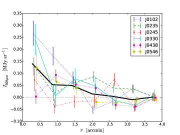
Figure 5.— $500\,\rm\mu m$ SZE radial profiles for clusters with Herschel SPIRE coverage. Profiles are extracted from maps after isolating the SZE signal component (Section 3.7), Fourier filtering the resulting map to mimic the LABOCA transfer function, and extracting point-like sources using the source extraction algorithm from Section 4.1. The thick black line represents the mean profile.

To test the reliability of our data reduction pipeline and source extraction algorithm, we compared our $250\,\rm\mu m$ integral number counts to those from the Herschel Multi-tiered Extragalactic Survey (HerMES; Oliver et al., 2010). Because our point-source removal technique breaks up $350$ and $500\,\rm\mu m$ sources and divides their flux among multiple $250\,\rm\mu m$ counterparts, our number counts for $350$ and $500\,\rm\mu m$ cannot be meaningfully compared to those of Oliver et al. (2010). We can however compute the number density of sources with $S_{250}>100\,\rm mJy$ around all clusters with Herschel SPIRE data except ACT-CL J0330-5227, which has significantly reduced sensitivity, also masking within $5^{\prime}$ radii of the cluster centers to avoid the effects of gravitational lensing. At these bright flux densities where completeness corrections will be minimal, we find $N_{>100\,\rm mJy}=8.0\pm 4.0\,\rm deg^{-2}$, in agreement with the results from Oliver et al. (2010) who find $N_{>100\,\rm mJy}=12.8\pm 3.5\,\rm deg^{-2}$.

4. Point source contamination

4.1. SMGs

In the iteratively reduced LABOCA images, we find bright SMGs superposed on the clusters’ extended SZE emission. A complete analysis of the statistical properties of the detected SMGs and their multi-wavelength counterparts will be presented in a forthcoming paper (Aguirre et al., in prep). Here we only consider the SMGs nearest to the clusters and study how their presence affects the measured SZE signals.

SMGs are extracted from the iterative multi-scale LABOCA map (Section 3.1.3) of a given cluster using the following process. First, SMG locations are found by using a spatial matched filter (Serjeant et al., 2003) to search for sources shaped like the ideal telescope PSF within an unsharp-masked version of the map. The unsharp mask uses a median filter with a kernel size of $3\times\rm FWHM$, and allows for point sources to be disentangled from the diffuse large spatial-scale SZE signals near the cluster centers. Next, we measure the flux density of each detected SMG by fitting the original (non un-sharp masked) data at the source’s location with an ideal PSF while holding the position fixed and varying the flux density and a non-negative background offset.

We detect a total of 36 $\rm S/N>4$ point sources within $\theta_{500c}$ of our 11 cluster centers, giving an estimated total flux density per cluster in high-significance SMGs of $46^{+24}_{-32}\,\rm mJy$. Using the combined area of $0.10\,\rm deg^{2}$, this sample has cumulative number counts of $>10\,\rm mJy$ SMGs of $N(>10\,{\rm mJy})=223\pm 49\,\rm deg^{-2}$, 6–10 times greater than those of sources with comparable brightness in blank fields (Weiß et al., 2009). Due to the negative k-corrections and high redshifts of SMGs, the number density enhancement is likely due to gravitational lensing by the clusters’ potentials. Gravitational lensing does not alter the average integrated flux density of the projected SMG population, but it does increase the Poisson “shot noise” variance (e.g., Refregier & Loeb, 1997), and could introduce a bias in flux-constrained (i.e., either a S/N threshold or upper limit) aperture photometry near vs. away from clusters.

The $345\,\rm GHz$ flux density in bright SMGs inside the smaller apertures used in our analysis of the SZE (Section 5) is $26_{-26}^{+21}\,\rm mJy$, corresponding to $6\pm 5\,\rm mJy$ at $218\,\rm GHz$ and $2\pm 2\,\rm mJy$ at $148\,\rm GHz$. The scaling to lower frequencies is done using a modified Planck function with parameters $\beta=1.5$ and $T_{\rm D}=37.4\,\rm K$, values for typical blank-field $345\,\rm GHz$-selected SMGs (Wardlow et al., 2011). The contaminating SMG signal represents $18\%$ of the SZE signal per cluster at $345\,\rm GHz$, and $2\%$ at $148\,\rm GHz$, respectively. The contaminating SMGs are subtracted from the maps before further analysis of the SZE signals.

4.1.1 El Gordo and “La Flaca”

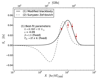
Figure 6.— Observed photometry and best-fit thermal and SZE spectra for J010256$-$491509 (“La Flaca”). From left to right, the red points represent LABOCA $345\,\rm GHz$ and SPIRE $500\,\rm\mu m$, $350\,\rm\mu m$, and $250\,\rm\mu m$ data. The solid black line represents the least-squares fit to the data using a modified blackbody spectrum with fixed parameters $T_{d}=37.4\,\rm K$ and $\beta=1.5$, which are adopted from Wardlow et al. (2011). The best fit redshift and infrared luminosity are $z=4.09$ and $L_{\rm IR}=3.19\times 10^{12}\,L_{\odot}$. The dashed curve represents the best-fitting thermal SZE SED assuming $T_{e}=25\,\rm keV$, which is formally unsatisfactory.

El Gordo (ACT-CL J0102-4915) has two bright point sources projected at small clustercentric radii; the brighter of the two ($S_{\nu}=36\pm 2\,\rm mJy$) we refer to as “La Flaca.” We briefy describe La Flaca’s properties here because it is exceptionally bright (The next brightest SMG within our sample has flux density $\sim 27\,\rm mJy$ and is located in ACT–CL J0438-5419), second in brightness only to the lensed SMG (Wilson et al., 2008; Johansson et al., 2010, e.g.) behind the Bullet cluster (ACT-CL J0658-5557). La Flaca is located at $\alpha=15.732207^{\circ}$ $\delta=-49.252415^{\circ}$ and has an extremely faint radio counterpart with $S_{2.1}=24\pm 7\,\rm\mu Jy$. To test the possibility that La Flaca is a local SZE enhancement, we compare the spectral fits of the source’s LABOCA+SPIRE photometry using a modified black body spectrum and thermal SZE spectrum. Figure 6 shows the best-fit curves for each model. We find that the SZE spectral shape is incompatible with the data; thus, La Flaca is more likely to be a high-redshift dusty star-forming galaxy than a compact SZE enhancement.

The best-fit modified Planck function parameters are $z=4.1$ and $L_{\rm IR}=3.2\times 10^{12}\,L_{\odot}$, assuming the median observed $T_{\rm D}=37.4\,K$ and $\beta=1.5$ from the LABOCA Extended-CDFS SMG survey (LESS; Wardlow et al., 2011). Using the $610\,\rm MHz$ GMRT data (Lindner et al., 2014), we derive a radio spectral index of $\alpha\sim-1.3$, giving a redshift estimate of $z=4.0$ based on the radio-to-far IR spectral index (Carilli & Yun, 1999), in agreement with that of the spectral fit and further supporting the conclusion that La Flaca is a high-redshift SMG.

There are two faint HST sources within $1^{\prime\prime}$ of La Flaca’s 345 GHz centroid. The brighter source has magnitude $m_{775}=23.8$ and resembles a spiral galaxy, and the fainter source has magnitude $m_{775}=26.8$ and is unresolved. La Flaca is also only a few arcseconds away from the positions of gravitational lensing critical curves for background galaxies between $z=4$–9 (Zitrin et al., 2013a).

4.2. Radio sources

Radio and IR-bright sources can potentially “fill in” SZE decrement signals and artificially enhance SZE increment signals in the $1.5^{\prime}$-resolution SZE maps typically used to detect clusters. With our high-resolution $2.1\,\rm GHz$ and $345\,\rm GHz$ imaging, we can disentangle the signals of point sources from those of the true SZE signal, allowing us to derive more robust measurements of the thermal and kinetic SZE signals. In this section, we quantify the degrees of radio and submillimeter contamination of the SZE signal.

4.2.1 $2.1\,\rm GHz$ number counts

We use the Common Astronomy Software Applications (CASA; McMullin et al., 2007) task findsources to fit elliptical Gaussian profiles to all bright sources in the ATCA maps down to a significance of $4\sigma$ and out to the $10\%$ primary beam power radius ($22^{\prime}$). We adopt a primary beam profile based on the effective mean frequency of each observation (see Table 4). To minimize radial selection bias, we only consider sources that have primary beam-corrected flux densities above the detection threshold at all radii, i.e., $>4\sigma/0.1=400\,\rm\mu Jy$. Additionally, only compact sources that have major and minor FWHMs, $a$ and $b$, satisfying $a<3\rm\times FWHM^{\rm beam}_{\rm maj}$, $b>0.5\times\rm FWHM^{\rm beam}_{\rm min}$, and $a/b<1.5\times\rm FWHM^{\rm beam}_{\rm maj}/FWHM^{\rm beam}_{\rm min}$ are kept. We consider only compact sources because extended radio sources like jets and lobes from active galactic nuclei have steep radio spectral indices and will therefore contribute negligibly in the frequency range $\nu\geq 148\,\rm GHz$. These criteria result in a total for all clusters of 1934 radio sources with flux densities between $28\,\rm\mu Jy$ and $1.65\,\rm Jy$.

Fainter sources have an increased chance of having their flux densities scattered below the detection threshold by noise, thus lowering their completeness. Because the noise in the $2.1\,\rm GHz$ maps is nearly Gaussian, we correct for completeness using an analytic correction in the following way. The completeness probability, $C$, that a source with true flux density $S_{\nu}$ will be detected above a threshold of $N\,\sigma$ is given by

$$C=1-\Phi\left(\frac{N\sigma-S_{\nu}}{\sigma}\right),$$ (10)

where $\Phi(x)$ is the cumulative normal distribution function. The completeness correction is then implemented by computing number counts using a weighted histogram with weights $w_{i}=C_{i}^{-1}$.

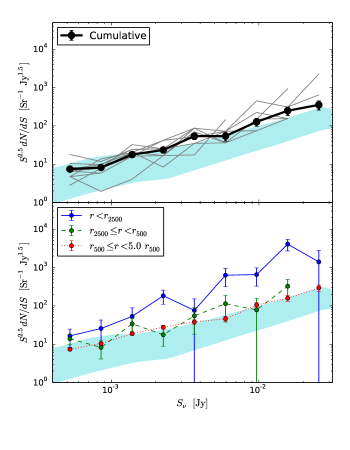
Figure 7.— $2.1\,\rm GHz$ number counts. Upper panel Total $2.1\,\rm GHz$ differential number counts towards the clusters out to a maximum search radius of $r_{\rm max}=10^{\prime}$. The grey lines represent the counts around individual clusters. The thick black line represents the cumulative counts across all clusters. The black circles mark the centers of the bins, which are logarithmically spaced between $400\,\rm\mu Jy$ and $31\,\rm mJy$. Lower panel: $2.1\,\rm GHz$ differential number counts as a function of physical clustercentric projected radius. The connected points and error bars represent number counts and Poisson uncertainties inside a circle with projected radius $r\leq r_{2500c}$ (solid), inside an inner annulus with radii $r_{2500c}<r\leq r_{500c}$ (dashed), and inside an outer annulus with radii $r_{500c}<r<5.0\,r_{500c}$ (dotted). In all panels, the shaded blue area shows the $95\%$ confidence region of ATCA $20\,\rm cm$ number counts in the AKARI Deep Field South from White et al. (2012). We use the conversion $r_{2500c}\simeq 0.44\,r_{500c}$ (Arnaud et al., 2010).

Figure 7 (upper panel) shows combined and individual $2.1\,\rm GHz$ number counts in nine log-spaced flux density bins. The power-law index of the counts $\delta$, where $dN/dS\propto S^{-\delta}$, is $\delta\simeq 1.7$. We next compute the number counts in three disjoint regions defined relative to the clusters’ physical radii, and find that the counts in the $\theta<\theta_{2500c}$ region are elevated (especially at high flux densities) compared to the more distant regions (Figure 7 lower panel), in agreement with a previous radio survey of southern X-ray selected clusters (Slee et al., 2008). This enhanced source density in cluster interiors is likely due to the presence of both radio-loud cluster member galaxies and (possibly at a lower level) gravitationally lensed background AGNs and star-forming galaxies. We have also checked for variation in the counts for the top, bottom, left, and right halves of the radio images and find no significant differences.

4.2.2 Radio contamination extrapolated to $148\,\rm GHz$

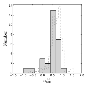
Figure 8.— Spectral index $\alpha^{2.1}_{610}$ of 28 pairs of $>4\sigma$ significance $2.1\,\rm GHz$ and $610\,\rm MHz$ sources within $6^{\prime}$ of the center of ACT-CL J0102$-$4915. The median and interquartile range are $\alpha^{2.1}_{610\,\rm median}=0.56$ and 0.37–0.69, respectively. For comparison, the grey dashed line shows the $\rm 1.4\,\rm GHz/330\,\rm MHz$ spectral index distribution of radio sources detected from deep observations of the Lockman Hole North (Owen et al., 2009).

We use our $610\,\rm MHz$ Giant Metre-wave Radio Telescope (GMRT) image of ACT-CL J0102$-$4915 (Lindner et al., 2014) to compute the radio spectral index $\alpha^{2.1}_{610}$ distribution of $2.1\,\rm GHz$ sources, which allows us to extrapolate their flux densities to the higher frequencies of the SZE decrement. We find 28 $2.1\,\rm GHz$/$610\,\rm MHz$ pairs of sources with $<1^{\prime\prime}$ ($7.8\,\rm kpc$) separation and $>4\sigma$ significance out to a $6^{\prime}$ radius relative to the SZE decrement centroid, and compute their spectral indices as

$$\alpha^{2.1}_{610}=-\log(S_{2.1}/S_{610})/\log(2.1/0.610).$$ (11)

The distribution $\alpha^{2.1}_{610}$ is shown in Figure 8. We find a median spectral index $\alpha^{2.1}_{610\,\rm median}=0.56$ with interquartile range 0.37–0.69. Only $4.9\%$ of $>4\sigma$ ATCA radio sources have optically-selected cluster member counterparts (for the clusters that overlap between the two samples) from Sifón et al. (2013). The disjoint source catalogs along with the fact that our spectral index distribution is similar to that of Owen et al. (2009) indicates that radio source contamination in our clusters is due mostly to foreground and background galaxies, allowing us to use the spectral index distribution measured in the field of ACT-CL J0102-4915 to predict the 148 GHz contamination in our full cluster sample. The recent study of the average submillimeter emission associated with 1.4 GHz-selected AGN by Gralla et al. (2014) finds that a low-frequency estimate of average AGN spectral index remains valid when extrapolating all the way to $218\,\rm GHz$, validating our extrapolation of 2.1 GHz emission up to the ACT bands at 148 and 218 GHz.

Because we only measure the spectral indices of sources that are detected at both $610\,\rm MHz$ and $2.1\,\rm GHz$, we check for sources with flat/inverted spectral indices that may not be detected at $610\,\rm MHz$ but could be bright at $2.1\,\rm GHz$ and higher frequencies by searching for $20\,\rm GHz$ counterparts to our ATCA and GMRT detections using the Australia Telescope $20\,\rm GHz$ survey (AT20G; Murphy et al., 2010). There is one match between the AT20G catalog (Murphy et al., 2010) and our ATCA and GMRT sources. The source lies $15^{\prime}$ away from the center of cluster ACT-CL J0215-5212 and has $S_{20}=0.11\pm 0.01\,\rm Jy$ and $S_{2.1}=0.011867\pm 0.001726\,\rm Jy$, giving an inverted spectral index of $\alpha=1.0$. This source is only $10^{\prime\prime}$ away from a much brighter ATCA source with $S_{2.1}=0.897\pm 0.001\,\rm Jy$.

We detect 346 $2.1\,\rm GHz$ sources with $S_{2.1}>4\sigma$ within $\theta_{500c}$ of our ten clusters with ATCA imaging, corresponding to a mean $2.1\,\rm GHz$ flux density within $\theta_{500c}$ per cluster of $39^{+6}_{-6}\,\rm mJy$. After scaling the flux density to the $148\,\rm GHz$ SZE decrement using $\alpha^{2.1}_{610\,\rm median}=0.56$ and including an additional uncertainty based on the variation in the spectral index between the extremes of the interquartile range, the typical contaminating radio signal from $2.1\,\rm GHz$-detected synchrotron radio sources is estimated to lie between 2.1–$8.1\,\rm mJy$ in the $148\,\rm GHz$ SZE decrement.

Inside the photometric apertures used to constrain the clusters’ peculiar velocities (Section 5), radio sources contribute $28\pm 8\,\rm mJy$, corresponding to $3\pm 1\,\rm mJy$ at $148\,\rm GHz$, which is $3\%$ of the typical decrement signal in our sample.

5. Peculiar velocities

In addition to its Hubble-flow velocity, a galaxy cluster can have a velocity offset with respect to its local CMB rest-frame, known as its peculiar velocity $v_{p}$. As well as being interesting in its own right as a statistical cosmological probe of large-scale structure (e.g., Doré et al., 2003), $v_{p}$ introduces a frequency-independent temperature fluctuation known as the kinetic SZ (kSZ; Equation 3.6), in contrast to the frequency-dependent SZ signal due to thermal motion of the electrons in the cluster (tSZ; Equation 6). This kSZ contribution can therefore affect the scaling between thermal $Y_{\rm SZ}$ and cluster mass.

Mroczkowski et al. (2012) report that their $268\,\rm GHz$ data for the triple-merger cluster MACS J0717.5$+$3745 adequately fit their SZE model only if they allow for a strong kSZ distortion from a high-velocity subcomponent. It is unclear whether strong kSZ distortions like those seen by Mroczkowski et al. (2012) are common in merging clusters. Recent results from Planck Collaboration et al. (2014d) only constrain the RMS fluctuations in $v_{p}$ to be $\leq 800\,\rm km\,s^{-1}$ (95% confidence) for a sample from the Meta Catalogue X-ray Detected Clusters (Piffaretti et al., 2011). If transient kSZ distortions are common in merging cluster systems, then the $Y_{\rm SZ}$–mass relation in SZE clusters may be significantly affected. As a cautionary indicator here, Sifón et al. (2013) find at least one indication of dynamical activity in $81^{+19}_{-22}\%$ (13/16) of a representative sample of ACT clusters (nine of which overlap with this paper’s sample).

We use our point source-subtracted multi-band data to constrain the peculiar velocities of our targets by parametrizing the observed SZE signal with $v_{p}$ and an integrated SZE signal $Y^{\prime}_{\rm SZ}$. The iterative pipeline (Section 3.1.2) faithfully recovers extended emission only up to angular scales of $\sim 2^{\prime}$, while $\theta_{500c}$ values can be much larger. Therefore, to strengthen constraints while fitting for $v_{p}$, we choose circular apertures for each cluster (typically 1.5–$2^{\prime}$ radii) that contain the observed scale of emission in the $345\,\rm GHz$ images. $Y^{\prime}_{\rm SZ}$ is therefore the effective integrated SZ signal within each of these apertures, and a lower limit on $Y_{\rm SZ}(\theta\leq\theta_{500c})$. We have recently obtained Chandra imaging (PI: Hughes) for many clusters in our sample and use these data to independently measure $T_{e}$ in these systems (Hughes et al. in prep). The systematic errors due to the different weighting between the X-ray-derived electron temperatures ($\propto n_{e}^{2}$) and the optical depth-weighted electron temperatures used in the calculations of the SZ effect are expected to be only $10$–$20\,\rm km\,s^{-1}$ (Sehgal et al., 2005). For the current analysis, we set $k_{\rm B}T_{e}=5\,\rm keV$ (see Table 2) for clusters with unknown gas temperatures.

For each integrated flux density measurement $S_{\rm SZ,i}$ at $x_{i}=h\,\nu_{i}/k_{\rm B}T_{e}$ we compute the expected SZE signal $S^{\rm model}_{\rm SZ}(Y_{\rm SZ}^{\prime},x_{i},v_{p},T_{e})$. We fit the data to the multi-band model using a grid-based search. The noise in all images is nearly Gaussian, and therefore the conditional probability density of obtaining measurements $S_{{\rm SZ},i}$, given the model parameters $\theta=(Y^{\prime}_{\rm SZ},v_{\rm pec})$ is

$$p_{i}(x_{i};\theta)\propto e^{-(S_{{\rm SZ},i}-S_{{\rm SZ},i}^{\rm model})^{2}/2\sigma_{i}^{2}}.$$ (12)

The joint probability density of obtaining all measurements is then given by $P(x;\theta)\propto\Pi_{i}p_{i}$. We take as the best-fit parameters those that maximize the likelihood function, and the final quoted $1\sigma$ uncertainties in $v_{p}$ and $Y_{\rm SZ}^{\prime}$ are found by marginalizing over the 2D likelihood parameter space and integrating the resulting 1D probability functions within iso-contours to contain $\pm 68\%$ probability. The best-fit peculiar velocities and corresponding $68.2\%$ confidence intervals are presenting in Table 2.

At 148 and 345 GHz, the SZE signal is much brighter than the background confusion noise. The situation is reversed for 350 and $500\,\rm\mu m$, where great efforts must be made to extract the SZE signal from the strong SMG background (i.e., see Section 3.7). Recent work by Zemcov et al. (2013) has shown that by subtracting bright submillimeter point sources near massive clusters, one will produce a deficit in the surface brightness of the local cosmic infrared background compared to an off-cluster sky region. By subtracting point-sources at a level comparable to that used in Section 3.7, Zemcov et al. (2013) find a typical intensity deficit of $\sim 0.5\,\rm MJy\,sr^{-1}$ in the cores of four massive clusters. This may related to why our SPIRE $500\,\mu\rm m$ photometry is systematically low compared to the other bands (see Figure 9). Because of this extra uncertainty in the SPIRE photometry, we present peculiar velocity fits for individual clusters both including and excluding the SPIRE data points (Table 2); other sample-wide properties are computed with only ACT + LABOCA photometry. Figure 9 shows the best-fit SZE spectra for all clusters, with the $\chi^{2}$ per degree of freedom ($\chi^{2}/\nu$) and $p$ values indicated in the panels.

The mean peculiar velocity of the sample is $\left<v_{p}\right>=153\pm 383\,\rm km\,s^{-1}$, consistent with the limit of $72\pm 60\,\rm km\,s^{-1}$ found by Planck Collaboration et al. (2014d) using the variance of the CMB towards X-ray detected clusters. The measured peculiar velocity dispersion of the clusters in our sample is $1449\,\rm km\,s^{-1}$, and represents an upper limit to the intrinsic peculiar velocity dispersion.

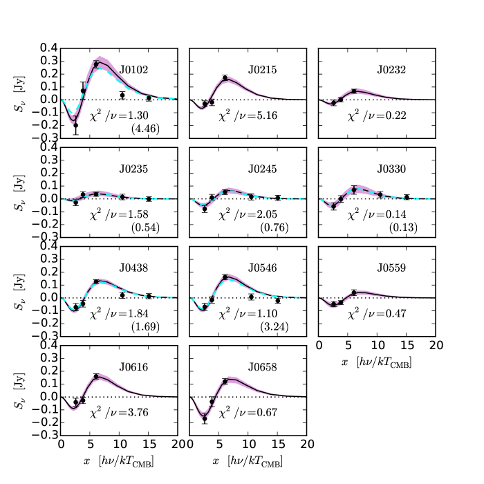
Figure 9.— Best-fit SZE spectra for all 11 clusters in our sample. The solid black curve and purple region show the best-fit model and 68% confidence region for 148, 218, and $345\,\rm GHz$ photometry and the dashed red line shows the best-fit model when including the Herschel SPIRE bands at 250, 350, and $500\,\rm\mu m$. The fit quality ($\chi^{2}/\nu$) when using only ACT + LABOCA bands is indicated in the panels, with the corresponding value when including SPIRE photometry shown in parentheses. From left to right, the data points are ACT $148\,\rm GHz$, ACT$\,218\,\rm GHz$, LABOCA$\,\rm 345\,\rm GHz$, SPIRE $500\,\rm\mu m$ and SPIRE $350\,\rm\mu m$ (the latter two only for the six clusters with $Herschel$ observations) .

Halverson et al. (2009) find that the mass-weighted SZE-derived temperature measured for the Bullet cluster ($10.8\pm 0.9\,\rm keV$; Halverson et al., 2009) is significantly lower than that derived from the X-ray observations ($13.9\,\rm keV$; Govoni et al., 2004). This difference is caused by the different sampling functions for X-ray derived temperatures ($\propto\int n^{2}$) and SZE-derived temperatures ($\propto\int n$). We adopt the SZE-based temperature for the Bullet cluster from Halverson et al. (2009) and derive a large peculiar velocity of $3100^{+1900}_{-1500}\,\rm km\,s^{-1}$. This signal is unlikely to be caused by contamination of sources fainter than $S_{345}<10\,\rm mJy$, because positive signal contamination acts to push $v_{\rm pec}$ to more negative values. In the Bullet cluster, Markevitch (2006) find a central “bullet” collision velocity of $4700\,\rm km\,s^{-1}$. Our signal may be due to a kSZ distortion related to this high-velocity subcomponent, similar to the findings of Mroczkowski et al. (2012) for MACS J0717.5$+$3745.

5.1. Impact of $v_{\rm pec}$ on $Y_{SZ}$-$M$ scaling relations

We next compute $Y^{\prime 0}_{\rm SZ}$, the best-fit integrated SZ signal when the peculiar velocity is fixed at $v_{\rm pec}=0\,\rm km\,s^{-1}$, and define the systematic uncertainty due to non-zero $v_{\rm pec}$ as $\Delta Y_{\rm SZ}^{\prime}=\left<\left|Y_{\rm SZ}^{\prime}-Y_{\rm SZ}^{\prime 0}\right|\right>$. We use the $Y_{\rm SZ}-M$ scaling relation $M\propto Y_{sz}^{0.48\pm 0.11}$ from Sifón et al. (2013) to derive a relative systematic uncertainty in cluster mass due to the clusters’ peculiar velocities of $\left<\Delta M/M\right>=3.5\pm 0.8\%$. Because the fractional change in $\Delta I_{\rm SZ}$ due to a non-zero peculiar velocity is independent of the mean Compton parameter, our aperture-based estimate of the relative uncertainty in $Y_{\rm SZ}$ can be directly applied to cluster-integrated $Y_{\rm SZ}$ measurements.

5.2. Comparison to simulations

To understand the intrinsic scatter and systematic uncertainties in our derived values for $v_{\rm pec}$, we applied our technique of extracting $v_{\rm pec}$ (Section 5) to the realistic simulated cluster images from the all-sky maps of Sehgal et al. (2010). We use the “Full SZ” images at 148, 219, and $350\,\rm GHz$, which contain thermal and kinetic SZ signals from clusters, groups, and the intracluster medium. The large scale mass distribution is created using a dark matter N-body simulation with a comoving box size of $L=1000\,h^{-1}\,\rm Mpc$ (for details, see Sehgal et al., 2007, 2010). We cut out $0.3^{\circ}\times 0.3^{\circ}$ images around 100 simulated clusters that were randomly chosen among those with $z>0.3$ and $M_{\rm vir}>3\times 10^{14}\,M_{\odot}$. For each cluster image, we applied the Fourier-based LABOCA filtering, extracted the total flux densities at 148, 219, and 350GHz within a $1.5^{\prime}$ aperture centered on the central halo position, and performed the maximum likelihood fit from Section 5.

We find an intrinsic scatter in output $v_{\rm pec}$ of $\sigma_{v_{\rm pec}}=213\,\rm km\,s^{-1}$, and a bias of ($\left<v_{\rm pec,out}/v_{\rm pec,in}\right>-1$) of 0.36. For $0.25^{\prime}$ apertures, the scatter is $137\,\rm km\,s^{-1}$ and the median bias is 0.15. Given that the smaller apertures reduce the bias and scatter, we attribute both effects to the aperture-dependent irreducible error from assuming a single temperature and velocity throughout the volume of a cluster.

To investigate the source of the scatter and bias in more detail, we next performed an experiment exactly the same as above, except that we computed the photometry for each system while varying the relation between the gas temperature assumed in the maximum likelihood fit $T_{\rm fit}$, and the true gas temperature of the cluster $T_{\rm true}$. When $T_{\rm fit}=T_{\rm true}$, we find negligible scatter and bias, but for $T_{true}=0.8\,\times T_{fit}$, we find a median bias in the recovered peculiar velocity of 0.2. This induced temperature-related bias can explain the bias we see in the extracted $v_{\rm pec}$ of the simulated clusters above: in the simulations, $T_{\rm true}$ is measured in the 3D centers of the clusters, and larger apertures will include more cool gas at larger cluster-centric radii. This effect is also likely operating in the real observations since the X- ray-derived gas temperatures are weighted by $n_{e}^{2}$ and preferentially sample the dense interiors of clusters. This might explain, for example, the $22\%$ difference found by Halverson et al. (2009) in SZE- and X-ray-derived temperatures quoted above. Figure 10 shows the input and output peculiar velocities for each of the three numerical experiments above.

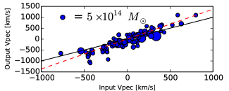
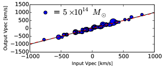
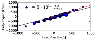
Figure 10.— Recovered (output) peculiar velocity as a function of known (input) peculiar velocity for a sample of 100 clusters with $z>0.3$ and $M_{\rm vir}>3\times 10^{14}\,M_{\odot}$ from the Sehgal et al. (2010) all-sky simulations of the microwave sky. Top panel: Photometry is realistically extracted from the simulated images using $1.5^{\prime}$-radius circular apertures and $T_{\rm fit}=T_{\rm true}$. Middle panel: Perfect photometry with $T_{\rm fit}=T_{\rm true}$. Bottom panel: Perfect photometry with $0.8\times T_{\rm fit}=T_{\rm true}$. In each panel, the solid black line shows a linear relation with unity slope, and the dashed red line shows the best least-squares fit of a line constrained to pass through the origin. The diameters of the symbols are proportional to the simulated cluster masses with the scale of $5\times 10^{14}\,M_{\odot}$ indicated at the upper left of each panel.

6. Comparison to previous work

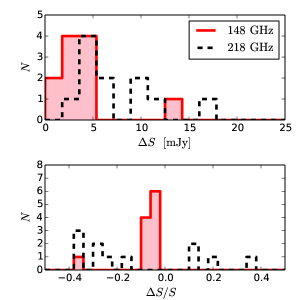
Figure 11.— 148 and 218 GHz absolute (above) and fractional (below) contamination of the SZ signal by SMGs and radio point sources. The varying sign of the $218\,\rm GHz$ fractional contamination ($\Delta S/S$) is caused by noise fluctuations because the clusters typically have small or negligible $218\,\rm GHz$ signals.

Figure 11 shows the combined absolute and relative contamination levels from radio sources and SMGs in our sample. Our results are in general agreement with previous predictions and measurements of radio and infrared source contamination at $148\,\rm GHz$. For example, based on simulations of the microwave sky, Sehgal et al. (2010) predicted that $<20\%$ of clusters with $M_{200c}>10^{14}\,M_{\odot}$ and $z<0.8$ should have their decrements filled in by $>50\%$. In our sample of clusters, we find a mean individual contamination fraction of $\left<\Delta S/S\right>=8\%$, and none with contamination $>50\%$.

Lima et al. (2010) presented analytic predictions of the Poisson variance in SZ flux density due to lensed background SMG populations. At 148 GHz, Lima et al. (2010) predict $\sigma_{\rm lensed\,SMG}\sim 2$–$3\,\rm mJy$ within $r_{2500c}$. Within our 1–$2^{\prime}$ radius apertures (similar to $r_{2500c}$ for our cluster sample), we estimate the RMS intensity of $148\,\rm GHz$ fluctuations due only to the significantly detected LABOCA point sources to be $2\,\rm mJy$.

Using 1.4, 30, and $140\,\rm GHz$ observations of 45 massive clusters, Sayers et al. (2013) estimate the fractional contamination due to radio sources to be $\simeq 20\%$ on average, with only 1/4 of clusters showing contamination greater than $1\%$. The mean individual contamination ($\left<\Delta S/S\right>$) by radio sources in our sample is 6%.

Benson et al. (2003) constrained the peculiar velocities of six clusters using the Sunyaev-Zel’dovich Infrared Experiment in three frequency bands between 150 and 350GHz, and placed a constraint on the intermediate Universe bulk flow velocity of $<1420\,\rm km\,s^{-1}$ (95% confidence), consistent with ours.

7. Conclusions

We present high-resolution $345\,\rm GHz$ LABOCA, $2.1\,\rm GHz$ ATCA (10 of 11) and $Herschel$ SPIRE (6 of 11) imaging of eleven massive SZE-selected clusters from the ACT southern survey (Marriage et al., 2011; Menanteau et al., 2010). We use these data to constrain the levels of radio source and SMG contamination of the SZE signals of the clusters, and also to constrain the cluster peculiar velocities using the kSZ effect.

We find that the contamination by $2.1\,\rm GHz$ radio sources of the $148\,\rm GHz$ SZE decrement is $3\pm 1\,\rm mJy$ per cluster, or $\sim$$3\%$ of the SZE decrement signal in our analysis. We measure the $2.1\,\rm GHz$ number counts in three disjoint regions around the clusters, $\theta<\theta_{2500c}$, $\theta_{2500c}<\theta<\theta_{500c}$, and $\theta_{500c}<\theta<5\,\theta_{500c}$, and find an enhancement in the counts for $\theta<\theta_{2500c}$.

The typical contamination from bright, unresolved SMGs is $26_{-26}^{+21}\,\rm mJy$ ($18\%$) per cluster at $345\,\rm GHz$, scaling to a $2\%$ effect on the $148\,\rm GHz$ decrement. The number counts of bright $S_{345}>10\,\rm mJy$ SMGs are $\sim 10\times$ greater than blank field measurements, likely due to gravitational lensing by the clusters’ potentials (as seen in, e.g., Knudsen et al., 2008; Johansson et al., 2011). The combined contamination by SMGs and radio sources ($\sim 5\%$ of the 148 GHz decrement signal on average) may contribute to, but still remains less than, the scatter found in the $Y_{\rm SZ}$-to-mass scaling relation of SZE clusters.

After subtraction of the bright SMGs, we use our multi-band data to constrain the peculiar velocities of the clusters. For clusters with high-significance SZE detections, the typical uncertainty in $v_{\rm pec}$ is $\pm 1000\,\rm km\,s^{-1}$, and for the full sample we find a mean peculiar velocity of $\left<v_{p}\right>=153\pm 383\,\rm km\,s^{-1}$. By comparing the best-fit $Y^{\prime}_{\rm SZ}$ values with and without fitting for $v_{\rm pec}$, we estimate that peculiar velocities introduce a scatter to the SZ-estimated mass of clusters at the level of $\left<\Delta M/M\right>=3.5\pm 0.8\%$.

Future observations with higher angular resolution and support for multiple instantaneous millimeter/submillimeter bandpasses can help reduce the uncertainties on $v_{\rm pec}$. Higher angular resolution can resolve a larger fraction of the CIB into point sources, and therefore reduce the magnitude of the remaining confused SMG background. The capability to observe multiple wavebands spanning the SZE decrement to the increment would allow the wavebands to be analyzed homogeneously, reducing the complexity of data reduction and related systematic uncertainties. These capabilities can be provided by wide-format multi-band bolometer cameras on telescopes like the Large Millimeter Telescope and the upcoming Cerro Chajnantor Atacama Telescope.

8. Acknowledgments

References

- Arnaud et al. (2010) Arnaud, M., Pratt, G. W., Piffaretti, R., et al. 2010, A&A, 517, A92
- Benson et al. (2003) Benson, B. A., Church, S. E., Ade, P. A. R., et al. 2003, ApJ, 592, 674
- Benson et al. (2013) Benson, B. A., de Haan, T., Dudley, J. P., et al. 2013, ApJ, 763, 147
- Blain et al. (2002) Blain, A. W., Smail, I., Ivison, R. J., Kneib, J.-P., & Frayer, D. T. 2002, Phys. Rep., 369, 111
- Bleem et al. (2014) Bleem, L. E., Stalder, B., de Haan, T., et al. 2014, ArXiv e-prints, arXiv:1409.0850
- Carilli & Yun (1999) Carilli, C. L., & Yun, M. S. 1999, ApJ, 513, L13
- Carlstrom et al. (2002) Carlstrom, J. E., Holder, G. P., & Reese, E. D. 2002, ARA&A, 40, 643
- Chluba et al. (2012) Chluba, J., Nagai, D., Sazonov, S., & Nelson, K. 2012, MNRAS, 426, 510
- Chluba et al. (2013) Chluba, J., Switzer, E., Nelson, K., & Nagai, D. 2013, MNRAS, arXiv:1211.3206
- Doré et al. (2003) Doré, O., Knox, L., & Peel, A. 2003, ApJ, 585, L81
- Duffy et al. (2008) Duffy, A. R., Schaye, J., Kay, S. T., & Dalla Vecchia, C. 2008, MNRAS, 390, L64
- Edge et al. (1994) Edge, A. C., Boehringer, H., Guzzo, L., et al. 1994, A&A, 289, L34
- Enoch et al. (2006) Enoch, M. L., Young, K. E., Glenn, J., et al. 2006, ApJ, 638, 293
- Fowler et al. (2007) Fowler, J. W., Niemack, M. D., Dicker, S. R., et al. 2007, Appl. Opt., 46, 3444
- Govoni et al. (2004) Govoni, F., Markevitch, M., Vikhlinin, A., et al. 2004, ApJ, 605, 695
- Gralla et al. (2014) Gralla, M. B., Crichton, D., Marriage, T. A., et al. 2014, MNRAS, 445, 460
- Griffin et al. (2010) Griffin, M. J., Abergel, A., Abreu, A., et al. 2010, A&A, 518, L3
- Güsten et al. (2006) Güsten, R., Booth, R. S., Cesarsky, C., et al. 2006, in Society of Photo-Optical Instrumentation Engineers (SPIE) Conference Series, Vol. 6267, Society of Photo-Optical Instrumentation Engineers (SPIE) Conference Series
- Halverson et al. (2009) Halverson, N. W., Lanting, T., Ade, P. A. R., et al. 2009, ApJ, 701, 42
- Hand et al. (2012) Hand, N., Addison, G. E., Aubourg, E., et al. 2012, Physical Review Letters, 109, 041101
- Hasselfield et al. (2013a) Hasselfield, M., Moodley, K., Bond, J. R., et al. 2013a, ApJS, 209, 17
- Hasselfield et al. (2013b) Hasselfield, M., Hilton, M., Marriage, T. A., et al. 2013b, J. Cosmology Astropart. Phys, 7, 8
- Jain & Lima (2011) Jain, B., & Lima, M. 2011, MNRAS, 411, 2113
- Johansson et al. (2011) Johansson, D., Sigurdarson, H., & Horellou, C. 2011, A&A, 527, A117
- Johansson et al. (2010) Johansson, D., Horellou, C., Sommer, M. W., et al. 2010, A&A, 514, A77
- Kitayama et al. (2004) Kitayama, T., Komatsu, E., Ota, N., et al. 2004, PASJ, 56, 17
- Knudsen et al. (2008) Knudsen, K. K., van der Werf, P. P., & Kneib, J.-P. 2008, MNRAS, 384, 1611
- Komatsu et al. (2001) Komatsu, E., Matsuo, H., Kitayama, T., et al. 2001, PASJ, 53, 57
- Komatsu et al. (2011) Komatsu, E., Smith, K. M., Dunkley, J., et al. 2011, ApJS, 192, 18
- Lima et al. (2010) Lima, M., Jain, B., & Devlin, M. 2010, MNRAS, 406, 2352
- Lindner et al. (2014) Lindner, R. R., Baker, A. J., Hughes, J. P., et al. 2014, ApJ, 786, 49
- Markevitch (2006) Markevitch, M. 2006, in ESA Special Publication, Vol. 604, The X-ray Universe 2005, ed. A. Wilson, 723
- Markevitch et al. (2002) Markevitch, M., Gonzalez, A. H., David, L., et al. 2002, ApJ, 567, L27
- Marriage et al. (2011) Marriage, T. A., Acquaviva, V., Ade, P. A. R., et al. 2011, ApJ, 737, 61
- Mason et al. (2010) Mason, B. S., Dicker, S. R., Korngut, P. M., et al. 2010, ApJ, 716, 739
- McMullin et al. (2007) McMullin, J. P., Waters, B., Schiebel, D., Young, W., & Golap, K. 2007, in Astronomical Society of the Pacific Conference Series, Vol. 376, Astronomical Data Analysis Software and Systems XVI, ed. R. A. Shaw, F. Hill, & D. J. Bell, 127
- Menanteau et al. (2010) Menanteau, F., González, J., Juin, J.-B., et al. 2010, ApJ, 723, 1523
- Menanteau et al. (2012) Menanteau, F., Hughes, J. P., Sifón, C., et al. 2012, ApJ, 748, 7
- Menanteau et al. (2013) Menanteau, F., Sifón, C., Barrientos, L. F., et al. 2013, ApJ, 765, 67
- Meneghetti et al. (2007) Meneghetti, M., Argazzi, R., Pace, F., et al. 2007, A&A, 461, 25
- Middelberg (2006) Middelberg, E. 2006, PASA, 23, 64
- Mroczkowski et al. (2012) Mroczkowski, T., Dicker, S., Sayers, J., et al. 2012, ApJ, 761, 47
- Murphy et al. (2010) Murphy, T., Sadler, E. M., Ekers, R. D., et al. 2010, MNRAS, 402, 2403
- Nord et al. (2009) Nord, M., Basu, K., Pacaud, F., et al. 2009, A&A, 506, 623
- Oliver et al. (2010) Oliver, S. J., Wang, L., Smith, A. J., et al. 2010, A&A, 518, L21
- Ott (2010) Ott, S. 2010, in Astronomical Society of the Pacific Conference Series, Vol. 434, Astronomical Data Analysis Software and Systems XIX, ed. Y. Mizumoto, K.-I. Morita, & M. Ohishi, 139
- Owen et al. (2009) Owen, F. N., Morrison, G. E., Klimek, M. D., & Greisen, E. W. 2009, AJ, 137, 4846
- Piffaretti et al. (2011) Piffaretti, R., Arnaud, M., Pratt, G. W., Pointecouteau, E., & Melin, J.-B. 2011, A&A, 534, A109
- Pilbratt et al. (2010) Pilbratt, G. L., Riedinger, J. R., Passvogel, T., et al. 2010, A&A, 518, L1
- Planck Collaboration et al. (2014a) Planck Collaboration, Abergel, A., Ade, P. A. R., et al. 2014a, A&A, 571, A11
- Planck Collaboration et al. (2014b) Planck Collaboration, Ade, P. A. R., Aghanim, N., et al. 2014b, A&A, 571, A20
- Planck Collaboration et al. (2014c) —. 2014c, A&A, 571, A29
- Planck Collaboration et al. (2014d) —. 2014d, A&A, 561, A97
- Poole et al. (2007) Poole, G. B., Babul, A., McCarthy, I. G., et al. 2007, MNRAS, 380, 437
- Poole et al. (2006) Poole, G. B., Fardal, M. A., Babul, A., et al. 2006, MNRAS, 373, 881
- Powell (1964) Powell, M. J. D. 1964, The Computer Journal, 7, 155
- Reese et al. (2012) Reese, E. D., Mroczkowski, T., Menanteau, F., et al. 2012, ApJ, 751, 12
- Refregier & Loeb (1997) Refregier, A., & Loeb, A. 1997, ApJ, 478, 476
- Reichardt et al. (2013) Reichardt, C. L., Stalder, B., Bleem, L. E., et al. 2013, ApJ, 763, 127
- Reynolds (1994) Reynolds, J. 1994, A Revised Flux Scale for the AT Compact Array
- Ruan et al. (2013) Ruan, J. J., Quinn, T. R., & Babul, A. 2013, MNRAS, 432, 3508
- Sault et al. (1995) Sault, R. J., Teuben, P. J., & Wright, M. C. H. 1995, in Astronomical Society of the Pacific Conference Series, Vol. 77, Astronomical Data Analysis Software and Systems IV, ed. R. A. Shaw, H. E. Payne, & J. J. E. Hayes, 433
- Sayers et al. (2013) Sayers, J., Mroczkowski, T., Czakon, N. G., et al. 2013, ApJ, 764, 152
- Scoville et al. (2007) Scoville, N., Aussel, H., Benson, A., et al. 2007, ApJS, 172, 150
- Sehgal et al. (2010) Sehgal, N., Bode, P., Das, S., et al. 2010, ApJ, 709, 920
- Sehgal et al. (2005) Sehgal, N., Kosowsky, A., & Holder, G. 2005, ApJ, 635, 22
- Sehgal et al. (2007) Sehgal, N., Trac, H., Huffenberger, K., & Bode, P. 2007, ApJ, 664, 149
- Sehgal et al. (2011) Sehgal, N., Trac, H., Acquaviva, V., et al. 2011, ApJ, 732, 44
- Serjeant et al. (2003) Serjeant, S., Dunlop, J. S., Mann, R. G., et al. 2003, MNRAS, 344, 887
- Sifón et al. (2013) Sifón, C., Menanteau, F., Hasselfield, M., et al. 2013, ApJ, 772, 25
- Siringo et al. (2009) Siringo, G., Kreysa, E., Kovács, A., et al. 2009, A&A, 497, 945
- Slee et al. (2008) Slee, O. B., Andernach, H., McIntyre, V. J., & Tsarevsky, G. 2008, MNRAS, 391, 297
- Sunyaev & Zel’dovich (1970a) Sunyaev, R. A., & Zel’dovich, Y. B. 1970a, Ap&SS, 7, 20
- Sunyaev & Zel’dovich (1970b) —. 1970b, Comments on Astrophysics and Space Physics, 2, 66
- Sunyaev & Zel’dovich (1972) —. 1972, Comments on Astrophysics and Space Physics, 4, 173
- Swetz et al. (2011) Swetz, D. S., Ade, P. A. R., Amiri, M., et al. 2011, ApJS, 194, 41
- Tucker et al. (1998) Tucker, W., Blanco, P., Rappoport, S., et al. 1998, ApJ, 496, L5
- Vanderlinde et al. (2010) Vanderlinde, K., Crawford, T. M., de Haan, T., et al. 2010, ApJ, 722, 1180
- Wardlow et al. (2011) Wardlow, J. L., Smail, I., Coppin, K. E. K., et al. 2011, MNRAS, 415, 1479
- Weiß et al. (2009) Weiß, A., Kovács, A., Coppin, K., et al. 2009, ApJ, 707, 1201
- White et al. (2012) White, G. J., Hatsukade, B., Pearson, C., et al. 2012, MNRAS, 427, 1830
- Wik et al. (2008) Wik, D. R., Sarazin, C. L., Ricker, P. M., & Randall, S. W. 2008, ApJ, 680, 17
- Wilson et al. (2008) Wilson, G. W., Hughes, D. H., Aretxaga, I., et al. 2008, MNRAS, 390, 1061
- Zel’dovich & Sunyaev (1969) Zel’dovich, Y. B., & Sunyaev, R. A. 1969, Ap&SS, 4, 301
- Zemcov et al. (2010) Zemcov, M., Rex, M., Rawle, T. D., et al. 2010, A&A, 518, L16
- Zemcov et al. (2013) Zemcov, M., Blain, A., Cooray, A., et al. 2013, ApJ, 769, L31
- Zhang et al. (2006) Zhang, Y.-Y., Böhringer, H., Finoguenov, A., et al. 2006, A&A, 456, 55
- Zitrin et al. (2013a) Zitrin, A., Menanteau, F., Hughes, J. P., et al. 2013a, ApJ, 770, L15
- Zitrin et al. (2013b) Zitrin, A., Meneghetti, M., Umetsu, K., et al. 2013b, ApJ, 762, L30