Stability of Switched Linear Systems under Dwell Time Switching with Piece Wise Quadratic Functions

Abstract

This paper provides sufficient conditions for stability of switched linear systems under dwell-time switching. Piece-wise quadratic functions are utilized to characterize the Lyapunov functions and bilinear matrix inequalities conditions are derived for stability of switched systems. By increasing the number of quadratic functions, a sequence of upper bounds of the minimum dwell time is obtained. Numerical examples suggest that if the number of quadratic functions is sufficiently large, the sequence may converge to the minimum dwell-time.

I Introduction

This paper investigates to the stability of switched linear systems:

$$\dot{x}(t)=A_{\sigma(t)}\,x(t),$$ (1)

where $x(t)\in\mathbb{R}^{n}$ is the state variable and $\sigma(t):\mathbb{R}^{+}\rightarrow\mathcal{I}_{N}:=\{1,\cdots,N\}$ is a time-dependent switching signal that indicates the current active mode of the system among $N$ possible modes in $\mathcal{A}:=\{A_{1},\cdots,A_{N}\}$. All matrices $A_{i},i=1,\cdots,N$ are assumed to be Hurwitz.

This class of systems has been widely investigated in the last decade, due to their importance both in the theoretical context and in engineering applications, see e.g. the recent surveys [1, 2, 3, 4].

The stability problem is one of the most important issue associated with the study of such systems. This problem has been addressed mainly using the theory of Lyapunov functions (LFs), to find conditions under which the system preserves stability. For example, the origin of system (1) is stable under arbitrary switching upon the existence of a common quadratic Lyapunov function [2], switched Lyapunov functions [5], multiple Lyapunov functions [1, 6], composite quadratic functions [7] or polyhedral Lyapunov functions [8, 9]. It is known that existence of a piece-wise linear (polyhedral) LF [8] or a piece-wise quadratic LF [10] is both necessary and sufficient for asymptotic stability of system (1) under arbitrary switching. This implies that the class of polyhedral functions or piece-wise quadratic functions are universal for characterization of stability of switched linear systems under arbitrary switching.

Another condition for stability is that based on dwell-time consideration. When all $A_{i}$’s are stable, stability of the origin can be ensured if the time duration spent in each subsystem is sufficiently long [2]. Upper bounds of the minimal dwell-time needed have also appeared [11, 12, 13, 14, 15]. Finding the minimum dwell time is known to be a hard problem and the research has been shifted to find testable conditions for the computation of upper bounds to the minimum dwell time. In [16] it is shown that stability under dwell time implies the existence of multiple Lyapunov norms, but the result is not constructive. In [12] a necessary and sufficient condition for stability of (1) in terms of piecewise linear (polyhedral) LF is provided, however construction of such polyhedral LF are not easy. Alternatively, [13, 17] introduce the concept of dwell-time(DT)-contractive sets and show that existence of a polyhedral DT-contractive set is both necessary and sufficient for stability of (1). An algorithm for computation of DT-contractive sets is also proposed for discrete-time systems, however computation of such sets for continuous systems is still lacking. In [14], polynomial functions are used to characterize the LF and the problem is formulated as a set of LMIs to compute upper bounds of minimum dwell time.

In this paper, we use piece-wise quadratic functions to characterize the Lyapunov functions and provide stability conditions in terms of bilinear matrix inequalities (BMIs). In the limiting case where the dwell-time approaches zero, system is under arbitrary switching, and the proposed conditions retrieve the results appeared in the literature [10]. Hence, this work can also be seen as a generalization of those obtained for arbitrary switching systems. It turns out by increasing the number of the quadratic functions that characterize the Lyapunov function, the proposed conditions has more degree of freedom and can be used to determine the minimal dwell-time needed for stability of (1).

The rest of this paper is organized as follows. This section ends with a description of the notations used. Section II reviews some standard terminology and results for switching systems. Section III shows the main results on the characterization of the Lyapunov functions with piece-wise quadratic functions for system (1). An algorithmic procedure for computation of sequence of upper bounds of the minimum dwell time needed for stability is also presented in this section. Sections IV and V contain, respectively, numerical examples and conclusions.

The following standard notations are used. $\mathbb{R}^{+}$ is the set of non-negative real numbers. Positive definite (semi-definite) matrix, $P\in\mathbb{R}^{n\times n}$, is indicated by $P\succ 0(\succeq 0)$ and $I_{n}$ is the $n\times n$ identity matrix. Given a $P\succ 0$, $\mathcal{E}(P):=\{x:x^{T}Px\leq 1\}$. Other notations are introduced when needed.

II Preliminaries

This section reviews definitions of dwell-time, admissible switching sequences, piece-wise quadratic functions and preliminary results on stability of (1) under dwell-time switching. These definitions have appeared in prior papers (see, e.g. [13, 18, 10, 14]) but are repeated here for completeness and for setting up the needed notations and results.

Denoting by $t_{k}$, $k=0,1,2,\cdots$ the switching instants, we assume that the following dwell-time restriction is imposed on the switching sequence $\sigma$, i.e. $\sigma\in\mathcal{S}_{\tau}$,

$$\mathcal{S}_{\tau}=\{\sigma(t):t_{k+1}-t_{k}\geq\tau\}$$ (2)

where $\mathcal{S}_{\tau}$ is the set of admissible switching signals that satisfies the dwell-time $\tau\geq 0$ restriction. Note that $\sigma(t)$ is a piecewise constant function, in the sense that $\sigma(t)=\sigma(t_{k})$ for $t\in[t_{k},t_{k+1})$. The minimum dwell-time, $\tau_{min}$, is defined as the minimum $\tau$ ensuring asymptotic stability of system (1) for all possible $\sigma\in\mathcal{S}_{\tau}$. More specifically, it is defined as

$$\tau_{min}:=\inf\{\tau\geq 0:(\ref{eqn:1a})\textrm{ is Asymptotically stable,}\forall\sigma(t)\in\mathcal{S}_{\tau}\}$$

II-A Piece-wise Quadratic Functions

For a positive semidefinite function $V:\mathbb{R}^{n}\rightarrow[0,\infty)$, denote its $1$-level set as

$$L_{V}:=\{x\in\mathbb{R}^{n}:V(x)\leq 1\}$$

The one sided directional derivative of $V(x)$ is defined with respect to two variables $x$ and $\zeta$, where $\zeta$ specifies the direction of increment or motion

$$\dot{V}(x;\zeta):=\lim_{h\downarrow 0}\frac{V(x+\zeta h)-V(x)}{h}$$

where $h\downarrow 0$ denotes decreasing to $0$.

Given $m$ positive definite matrices $P_{r}\succ 0$, $r=1,\cdots,m$, a piece-wise quadratic function can be obtained by [18]:

$$V_{max}(x):=\max\{x^{T}P_{r}\,x:r=1,\cdots,m\}$$ (3)

as the pointwise maximum of $m$ functions $x^{T}P_{r}x$, $r=1,\cdots,m$ and its 1-level set is the intersection of the ellipsoids $\mathcal{E}(P_{r})$, i.e. $L_{V_{max}}=\cap_{r=1}^{m}\mathcal{E}(P_{r})$.

The directional derivative of $V_{max}$ along the $i$-th mode of system (1) is [18]:

$$\dot{V}_{max}(x\,;A_{i}x):=\max\big{\{} x^{T}(A_{i}^{T}P_{s}+P_{s}A_{i})x:$$

$$s\in\{s:V_{max}(x)=x^{T}P_{s}\,x\}\big{\}}$$ (4)

II-B Stability Results

We start from the following theorem which states the necessary and sufficient condition for stability of (1) with dwell-time $\tau$.

Theorem 1.

[16] System (1) is asymptotically stable in $\mathcal{S}_{\tau}$, if and only if there exist continuous functions $V_{i}(x)$, associated to each mode $i$, such that

$$V_{i}(x)>0 \forall x\neq 0,\forall i$$ (5a)

$$\dot{V}_{i}(x\,;A_{i}x)<0 \forall x\neq 0,\forall i$$ (5b)

$$V_{j}(e^{A_{i}\tau}x)<V_{i}(x) \forall x\neq 0,\forall i\neq j$$ (5c)

The above theorem shows that stability of the system (1) the equivalent the existence of a mode-dependent Lyapunov function, $V_{\sigma(t)}(x)$, which is strictly decreasing for non-switching times, i.e. $t\neq t_{k}$, and it is strictly decreasing at the switching instances, i.e., $V_{\sigma(t_{k+1})}\big{(}x(t_{k+1})\big{)}<V_{\sigma(t_{k})}\big{(}x(t_{k})\big{)}$, however the the above theorem is not constructive. In [11], quadratic functions are used to characterize the $V_{i}$’s, but the conditions are only sufficient for stability. In [12], polyhedral (piece-wise linear) LFs are used to characterize the $V_{i}$’s and it is shown that piece-wise linear functions that satisfy condition (5) are both necessary and sufficient for stability of (1). However, the conditions obtained are nonlinear and cannot be solved efficiently. Motivated by the fact that piece-wise quadratic functions are universal for characterization of stability similar to piece-wise linear functions [18], the following section derives the stability conditions using piece-wise quadratic functions.

III Main Results

Given a positive integer $m$, a piece-wise quadratic function characterized by $m$ quadric functions is considered as the candidate Lyapunov function $V_{i}$ in Theorem 1, namely $V_{i}(x)=\max\{x^{T}P_{i,r}\,x:r=1,\cdots,m\}$, $i\in\mathcal{I}_{N}$. Using S-procedure, conditions of Theorem 1 can be converted into matrix inequalities. The following theorem provides a sufficient condition for stability of (1) under dwell-time switching.

Theorem 2.

Assume that, for a given $\tau>0$ and positive integer $m$, there exist scalars $\alpha_{irs}>0$, $\gamma_{jqirs}\geq 0$, $\sum_{s=1}^{m}\gamma_{jqirs}<1$ such that

$$P_{i,r}\succ 0\qquad\qquad\qquad\qquad\qquad\forall i,r=1,\cdots,m$$ (6)

$$A_{i}^{T}P_{i,r}+P_{i,r}A_{i}\prec\sum_{\begin{subarray}{c}s=1\\ s\neq r\end{subarray}}^{m}\alpha_{irs}(P_{i,s}-P_{i,r})$$

$$\qquad\qquad\qquad\qquad\qquad\qquad\qquad\forall i,r=1,\cdots,m$$ (7)

$$e^{A_{i}^{T}\tau}P_{j,\color[rgb]{0,0,1}q\color[rgb]{0,0,0}}\,e^{A_{i}\tau}\prec P_{i,r}+\sum_{\begin{subarray}{c}s=1\\ s\neq r\end{subarray}}^{m}\gamma_{jqirs}(P_{i,s}-P_{i,r})$$

$$\qquad\qquad\qquad\qquad\qquad\qquad\forall i\neq j,r=1,\cdots,m$$

$$\qquad\qquad\qquad\qquad\qquad\qquad\quad q=1,\cdots,m$$ (8)

Then, system (1) is asymptotically stable for every $\sigma\in\mathcal{S}_{\tau}$.

Proof.

Let $V_{i}(x)=\max\{x^{T}P_{i,r}\,x:r=1,\cdots,m\}$, $i\in\mathcal{I}_{N}$. We have to show that conditions 5(a)-(c) are satisfied. a) Obviously, (6) implies that $V_{i}(x)>0$ for all $x\neq 0$ and for all $i\in\mathcal{I}_{N}$. b) From (7) and (II-A), it follows that $\dot{V}_{i}(x;A_{i}x)<0$ for all $x\neq 0$ and for all $i\in\mathcal{I}_{N}$, see [18] for details. c) Without loss of generality consider $V_{j}(x)=\max\{x^{T}P_{j,q}\,x:q=1,\cdots,m\}$, $j\neq i$. We have to show that $V_{j}(e^{A_{i}\tau}x)<V_{i}(x)$. To this end, consider $(e^{A_{i}\tau}x)^{T}P_{j,q}\,(e^{A_{i}\tau}x)$ for any $q=1,\cdots,m$. For every $x$ such that $x^{T}P_{i,r}\,x\geq x^{T}P_{i,s}\,x$, $s=1,\cdots,m$, $V_{i}(x)=x^{T}P_{i,r}x$. This and (8) together impliy that

$$x^{T}(e^{A_{i}^{T}\tau}P_{j,q}\,e^{A_{i}\tau})x <\underbrace{x^{T}P_{i,r}x}_{V_{i}(x)}+\sum_{\begin{subarray}{c}s=1\\ s\neq r\end{subarray}}^{m}\gamma_{jqirs}\underbrace{x^{T}(P_{i,s}-P_{i,r})x}_{\leq 0}$$

$$<V_{i}(x)$$

Thus, $V_{j}(e^{A_{i}\tau}x)=\max_{q}\{x^{T}e^{A_{i}^{T}\tau}P_{j,q}\,e^{A_{i}\tau}x\}<V_{i}(x)$. The same argument holds for all the other regions where $x^{T}P_{i,r}\,x\leq x^{T}P_{i,s}\,x$. Hence conditions (5a)-(5c) of Theorem (1) are all satisfied and the proof is complete. ∎

Remark 1.

Note that, for $m=1$, $V_{i}(x)=x^{T}P_{i1}\,x$ and conditions (6)-(8) become: $P_{i,1}\succ 0,\,\forall i$,

$$A_{i}^{T}P_{i,1}+P_{i,1}A_{i}\prec 0 \forall i$$

$$e^{A_{i}^{T}\tau}P_{j,1}\,e^{A_{i}\tau}\prec P_{i,1} \forall i\neq j$$

and it retrieves the conditions appeared in [11].

For a given $m$, define $\tau_{[m]}$ as the smallest upper bound of $\tau_{min}$ guaranteed by Theorem 2, i.e.

$$\tau_{[m]}:=\inf\{\tau\geq 0:(\ref{eqn:7})-(\ref{eqn:9})\textrm{ hold}\}.$$

The following result provides a key property of the conditions of Theorem 2, which allows us to calculate $\tau_{[m]}$ via a bisection search where at each iteration the conditions (6)-(8) are tested.

Theorem 3.

Assume that (6)-(8) hold for some $\tau\geq 0$ and positive integer $m$. Then, conditions (6)-(8) hold for $\tau+\delta$ for any $\delta\geq 0$ with the same $m$.

Proof.

Suppose that (6)-(8) hold, and let $V_{i}(x)=\max\{x^{T}P_{i,r}\,x:r=1,\cdots,m\}$. Consider any $\delta\geq 0$. From (7) it follows that $\dot{V}_{i}(x;A_{i}x)<0$ and hence $V_{i}(x(\delta))<V_{i}(x(0))$ for every $x(0)$, which implies that $e^{A_{i}^{T}\delta}P_{i,r}e^{A_{i}\delta}\prec P_{i,r}$. Now, pre- and post-multiply (8) by $e^{A_{i}^{T}\delta}$ and $e^{A_{i}\delta}$ respectively. It follows that

$$e^{A_{i}^{T}(\tau+\delta)}P_{j,q}e^{A_{i}(\tau+\delta)} \prec e^{A_{i}^{T}\delta}P_{i,r}e^{A_{i}\delta}$$

$$+\sum_{\begin{subarray}{c}s=1\\ s\neq r\end{subarray}}^{m}\gamma_{jqirs}e^{A_{i}^{T}\delta}(P_{i,s}-P_{i,r})e^{A_{i}\delta}$$

$$\prec P_{i,r}+\sum_{\begin{subarray}{c}s=1\\ s\neq r\end{subarray}}^{m}\gamma_{jqirs}e^{A_{i}^{T}\delta}(P_{i,s}-P_{i,r})e^{A_{i}\delta}$$

Thus, $V_{j}(e^{A_{i}^{T}(\tau+\delta)}x)<V_{i}(x)$ and the theorem holds. ∎

Another important property of conditions of Theorem 2 that allows us to calculate $\tau_{[m]}$ is stated in the following lemma.

Lemma 1.

For a given $\tau$, suppose that conditions (6)-(8) are feasible for some $m$. Then, they are also feasible for $m+1$.

Proof.

Suppose a set of matrices $P_{i,r}\succ 0$, $r=1,\cdots,m$ satisfies conditions of Theorem 2 for a given $\tau$. A feasible solution for the case of $m+1$ is obtained by setting $P_{i,m+1}=P_{i,m}$, and keeping the rest of the $P_{i,r}$’s the same. ∎

An immediate conclusion of Lemma 1 and Theorem 3, is that the sequence of $\tau_{[m]}$, $m=1,2,\cdots$ is a non-increasing sequence and the limit $\bar{\tau}_{[m]}:=\lim_{m\rightarrow\infty}\tau_{[m]}$ exists. Obviously, $\bar{\tau}_{[m]}$ is an upper bound on the minimum dwell time, i.e. $\bar{\tau}_{[m]}\geq\tau_{min}$.

III-A Numerical Solution of Conditions of Theorem 2

The stability conditions (6)-(8) appeared in Theorem 2 are bilinear matrix inequalities with respect to variables $P_{i,r}$, $\alpha_{irs},\gamma_{jirs}$. Of course linearity is recovered if one fixes the matrices $P_{ir}$ or the scalars $\alpha$ and $\gamma$. Unfortunately, nested iterations by iteratively fixing $P_{ir}$ and computing proper values of $\alpha,\gamma$’s by means of convex optimization does not converge. In fact, it is known that finding the global solutions of BMI problems are NP-hard. We, however, find out that using the path-following method [19], we can find feasible solutions for the BMI conditions (6)-(8). The basic idea of path-following method is to use the first order approximation of the variables. To this end, we perturb the variables to $P_{ir}+\Delta P_{ir}$, $\alpha_{irs}+\Delta\alpha_{irs}$ and $\gamma_{jirs}+\Delta\gamma_{jqirs}$. Then, by ignoring the higher order terms, the conditions of Theorem 2 become:

$$P_{i,r}+\Delta P_{i,r}\succ 0$$ (9a)

$$A_{i}^{T}P_{i,r}+P_{i,r}A_{i}+A_{i}^{T}\Delta P_{i,r}+\Delta P_{i,r}A_{i}\prec\sum_{s\neq r}\Big{[}\alpha_{irs}(P_{i,s}-P_{i,r})$$

$$\qquad\quad+\alpha_{irs}(\Delta P_{i,s}-\Delta P_{i,r})+(P_{i,s}-P_{i,r})\Delta\alpha_{irs}\Big{]}$$ (9b)

$$e^{A_{i}^{T}\tau}P_{j,r}\,e^{A_{i}\tau}+e^{A_{i}^{T}\tau}\Delta P_{j,r}\,e^{A_{i}\tau}$$

$$\qquad\quad\prec\sum_{s\neq r}\Big{[}\gamma_{jqirs}(P_{i,s}+\Delta P_{i,s})+\Delta\gamma_{i,r,s}P_{i,s}\Big{]}$$ (9c)

For given $P_{ir},\alpha_{irs},\gamma_{jqigs}$ the above conditions are LMI with respect to variables $\Delta P_{ir},\Delta\alpha_{irs},\Delta\gamma_{jqirs}$.

One can start with a feasible solution to (6)-(8) and then solve (9a)-(9c) for $\Delta P_{ir},\Delta\alpha_{irs},\Delta\gamma_{jqirs}$. The next step is to update the scalars by letting $\alpha_{irs}\leftarrow\alpha_{irs}+\Delta\alpha_{irs}$ and $\gamma_{jirs}\leftarrow\gamma_{jqirs}+\Delta\gamma_{jqirs}$. Now by fixing these variables, (6)-(8) is an LMI in $P_{ir}$ and its feasibility can be checked efficiently. This iteration is then combined with a bisection search on $\tau$ to find the minimum $\tau_{[m]}$ for a given $m$. When $\tau_{[m]}$ cannot be improved with a fixed $m$, we increase the $m$ until $\tau_{[m+1]}=\tau_{[m]}$. Note that condition of Theorem 2 for $m=1$ is an LMI and the solution to that can be used for the initialization of the above iterative procedure.

IV Example

To illustrate the effectiveness of the proposed method, an examples is presented in this section. The example is taken from [12] where the system matrices are

$$A_{1}=\left[\begin{array}[]{cc}0&1\\ -10&-1\\ \end{array}\right],\;\;A_{2}=\left[\begin{array}[]{cc}0&1\\ -0.1&-0.5\\ \end{array}\right]$$

It has already been seen that for this system the minimum dwell time is 2.7078 [12]. The dwell-time obtained from method of [12] with a polyhedral characterization is $2.7420$. The sequence of the upper bounds of $\tau_{min}$ obtained from our proposed method is shown in Table I, where the minimum dwell time $\tau_{min}=2.70801$ can be obtained with $m=4$ quadratic functions. The $P_{ir}$ are reported here for verification:
$P_{11}=\left[\begin{array}[]{cc}196.665&17.322\\ &25.408\\ \end{array}\right]$, $P_{12}=\left[\begin{array}[]{cc}196.502&38.442\\ &12.137\\ \end{array}\right]$,
$P_{13}=\left[\begin{array}[]{cc}187.555&4.997\\ &19.280\\ \end{array}\right]$, $P_{14}=\left[\begin{array}[]{cc}196.502&38.455\\ &11.973\\ \end{array}\right]$,
$P_{21}=P_{22}=P_{23}=P_{24}=\left[\begin{array}[]{cc}137.512&177.991\\ &360.358\\ \end{array}\right]$

$m$	1	2	3	4	5
$\tau_{[m]}$	2.75090	2.70794	2.70782	2.70781	2.70781

TABLE I: The sequence of upper bounds of $\tau_{min}$

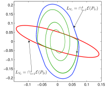
Figure 1: Level set of $V_{1},V_{2}$ for $m=4$.

Figure 1 shows the level-sets of the Lyapunov functions, i.e. $L_{V_{i}}=\cap_{r=1}^{4}\mathcal{E}(P_{ir})$ and a state trajectory from $x_{0}=(0.0689,0.0119)$ under periodic switching where $t_{k+1}-t_{k}=\tau_{[4]}$ and $\sigma(0)=1$. The Lyapunov function $V_{\sigma}(x(t))$ for this trajectory is also shown in Fig. 2(a). While $V_{\sigma}(x(t))$ increases at switching instants, the sequence of $V_{\sigma}(x(t_{k}))$ is monotonically decreasing (see Fig. 2(b)).

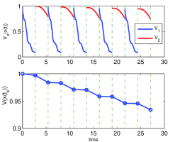
Figure 2: Illustration of $V_{\sigma}(x(t)),V_{\sigma}(x(t_{k}))$.

V Conclusions

Piece-wise quadratic functions are utilized to derive sufficient conditions for stability of switched linear systems under dwell-time switching. The stability conditions are in the form of bilinear matrix inequalities and are solved with path-following method. By increasing the number of quadratic functions, a sequence of upper bounds of the minimum dwell time is obtained. Numerical examples suggested that the conditions has the potential to be also necessary provided that the number of quadratic functions is sufficiently large. Further investigation is required to prove the necessity of the proposed conditions.

References

- [1] M. Branicky, “Multiple lyapunov functions and other analysis tools for switched and hybrid systems,” IEEE Trans. Automatic Control, vol. 43, no. 4, pp. 475–482, 1998.
- [2] D. Liberzon, Switching in Systems and Control. Birkhauser, Boston, 2003.
- [3] R. Shorten, F. Wirth, O. Mason, K. Wulff, and C. King, “Stability criteria for switched and hybrid systems,” SIAM Review, vol. 49, no. 4, pp. 545–592, 2007.
- [4] H. Lin and P. J. Antsaklis, “Stability and stabilizability of switched linear systems: A survey of recent results,” IEEE Trans. Automatic Control, vol. 45, no. 2, pp. 308–322, 2009.
- [5] J. Daafouz, P. Riedinger, and C. Iung, “Stability analysis and control synthesis for switched systems: a switched lyapunov function approach,” IEEE Trans. Automatic Control, vol. 47, no. 11, pp. 1883–1887, 2002.
- [6] M. Dehghan, “On the computation of domain of attraction of saturated switched systems under dwell-time switching,” in International Conference of Control, Dynamic Systems, and Robotics, 2014.
- [7] T. Hu, L. Ma, and Z. Lin, “Stabilization of switched systems via composite quadratic functions,” IEEE Trans. Automatic Control, vol. 53, no. 11, pp. 2571–2585, 2008.
- [8] F. Blanchini, S. Miani, and C. Savorgnan, “Stability results for linear parameter varying and switching systems,” Automatica, vol. 43, no. 10, pp. 1817–1823, 2007.
- [9] M. Dehghan, C.-J. Ong, and P. C. Y. Chen, “Enlarging domain of attraction of switched linear systems in the presence of saturation nonlinearity,” in ACC 2011, San Francisco, USA, 2011, pp. 1994–1999.
- [10] T. Hu and F. Blanchini, “Non-conservative matrix inequality conditions for stability/stabilizability of linear differential inclusions,” Automatica, vol. 46, no. 1, pp. 190–196, 2010.
- [11] J. C. Geromel and P. Colaneri, “Stability and stabilization of continuous-time switched systems,” SIAM Journal of Control and Optimization, vol. 45, no. 5, pp. 1915–1930, 2006.
- [12] F. Blanchini and P. Colaneri, “Vertex/plane characterization of the dwell-time property for switching linear systems,” in Decision and Control (CDC), 2010 49th IEEE Conference on, 2010, pp. 3258 –3263.
- [13] M. Dehghan and C.-J. Ong, “Discrete-time switched linear system with constraints: characterization and computation of invariant sets under dwell-time consideration,” Automatica, vol. 48, no. 5, pp. 964–969, 2012.
- [14] G. Chesi, P. Colaneri, J. Geromel, R. Middleton, and R. Shorten, “A nonconservative LMI condition for stability of switched systems with guaranteed dwell time,” IEEE Transactions on Automatic Control, vol. 57, no. 5, pp. 1297–1302, may 2012.
- [15] M. Dehghan and C.-J. Ong, “Characterization and computation of disturbance invariant sets for constrained switched linear systems with dwell time restriction,” Automatica, vol. 48, no. 9, pp. 2175–2181, 2012.
- [16] F. Wirth, “A converse lyapunov theorem for linear parameter varying and linear switching systems,” SIAM Journal on Control and Optimization, vol. 44, pp. 210–239, 2005.
- [17] M. Dehghan and C.-J. Ong, “Computations of mode-dependent dwell times for discrete-time switching system,” Automatica, vol. 49, no. 6, pp. 1804–1808, 2013.
- [18] T. Hu and Z. Lin, “Composite quadratic lyapunov functions for constrained control systems,” IEEE Transactions on Automatic Control, vol. 48, pp. 440–450, 2003.
- [19] A. Hassibi, J. How, and S. Boyd, “A path-following method for solving bmi problems in control,” in ACC, vol. 2, 2009, pp. 1385 – 1389.