Estimating parameters of a multipartite loglinear graph model via the EM algorithm

Abstract

We will amalgamate the Rash model (for rectangular binary tables) and the newly introduced $\alpha$-$\beta$ models (for random undirected graphs) in the framework of a semiparametric probabilistic graph model. Our purpose is to give a partition of the vertices of an observed graph so that the generated subgraphs and bipartite graphs obey these models, where their strongly connected parameters give multiscale evaluation of the vertices at the same time. In this way, a heterogeneous version of the stochastic block model is built via mixtures of loglinear models and the parameters are estimated with a special EM iteration. In the context of social networks, the clusters can be identified with social groups and the parameters with attitudes of people of one group towards people of the other, which attitudes depend on the cluster memberships. The algorithm is applied to randomly generated and real-word data.

1 Introduction

So far many parametric and nonparametric methods have been proposed for community detection in networks. In the nonparametric scenario, hierarchical or spectral methods were applied to maximize the two- or multiway Newman–Girvan modularity [1, 2, 3, 4]; more generally, spectral clustering tools, based on Laplacian or modularity spectra, proved to be feasible to find community, anticommunity, or regular structures in networks [5]. In the parametric setup, certain model parameters are estimated, usually via maximizing the likelihood function of the graph, i.e., the joint probability of our observations under the model equations. This so-called ML estimation is a promising method of statistical inference, has solid theoretical foundations [6, 7], and also supports the common-sense goal of accepting parameter values based on which our sample is the most likely.

In the 2010s, $\alpha$-$\beta$-models [8, 9] were developed as the unique graph models where the degree sequence is a sufficient statistic: given the degree sequence, the distribution of the random graph does not depend on the parameters any more (microcanonical distribution over the model graphs). This fact makes it possible to derive the ML estimate of the parameters in a standard way [10]. Indeed, in the context of network data, a lot of information is contained in the degree sequence, though, perhaps in a more sophisticated way. The vertices may have clusters (groups or modules) and their memberships may affect their affinity to make ties. We will find groups of the vertices such that the within- and between-cluster edge-probabilities admit certain parametric graph models, the parameters of which are highly interlaced. Here the degree sequence is not a sufficient statistic any more, only if it is restricted to the subgraphs. When making inference, we are partly inspired by the stochastic block model, partly by the Rasch model, the rectangular analogue of the $\alpha$-$\beta$ models.

The first type of block models is the homogeneous one: the probability to make ties is the same within the clusters or between the cluster-pairs. Although this probability depends on the actual cluster memberships, given the memberships of the vertices, the probability that they are connected is a given constant (parameter to be estimated). This stochastic block model, sometimes called generalized random graph or planted partition model, is thoroughly discussed in [11, 12, 13, 14, 15].

Here we propose a heterogeneous block model by carrying on the Rasch model developed more than 50 years ago for evaluating psychological tests [16, 17]. Given the number of clusters and a classification of the vertices, we will use the Rasch model for the bipartite subgraphs, whereas the $\alpha$-$\beta$ models for the subgraphs themselves, and process an iteration (inner cycle) to find the ML estimate of their parameters. Then, based on the overall likelihood, we find a new classification of the vertices via taking conditional expectation and using the Bayes rule. Eventually, the two steps are alternated, giving the outer cycle of the iteration. Our algorithm fits into the framework of the EM algorithm, the convergence of which is proved in exponential families under very general conditions [18, 7]. The method was originally developed for missing data, and the name comes from the alternating expectation (E) and maximization (M) steps, where in the E-step (assignment phase) we complete the data by substituting for the missing data via taking conditional expectation, while in the M-step (estimation phase) we find the usual ML estimate of the parameters based on the so completed data. The algorithm naturally extends to situations, when not the data itself is missing, but it comes from a mixture, and the grouping memberships are the missing parameters. This special type of the EM algorithm developed for mixtures is often called collaborative filtering [19, 20] or Gibbs sampling [21], the roots of which method can be traced back to [22]. In the context of social networks, the clusters can be identified with social strata and the parameters with attitudes of people of one group towards people of the other, which attitude is the same for people in the second group, but depends on the individual in the first group. The number of clusters is fixed during the iteration, but an initial number can be obtained by spectral clustering tools. Together with the proof of the convergence, the algorithm is applied to randomly generated and real-word data.

This kind of model building is originated both in the statistics literature, e.g., [23, 24, 25] and in the physics literature, e.g., [2, 26, 27]. In [28], the author already considers mixing according to vertex degree. In [13] the authors introduce the degree-corrected variant of the stochastic block model, but they use Poisson edge-probabilities. In [27] the likelihood, depending on Poisson parameters, is maximized with the trick that first a likelihood maximization is performed, then the problem is traced back to the minimum-cut objective. This is not the EM algorithm, though the idea of mixed tools resembles that.

In [29], without giving an algorithm, the authors maximize the so-called likelihood modularity over $k$-partitions of vertices, for given $k$. This is rather a non-parametric way of model fitting, since, instead of parameters, they substitute the relative frequency of the edges for their Bernoulli parameters, and theoretically maximize their profile likelihood with respect to the memberships of the vertices, which is considered as unknown parameter. They also prove the consistency of their estimates. [30] considers bipartition and multipartition of dense graphs with arbitrary degree distribution. In [15], based on the adjacency matrix as a statistical sample, the authors estimate the underlying partition of the vertices, given an upper bound for the number of blocks, in the stochastic block model. They prove that the suitably modified spectral partitioning procedure is consistent. Before fitting a model, its complexity may also be investigated. In [31], the authors give the quantification of the intrinsic complexity of undirected graphs and networks, via distinguishing between randomness complexity and statistical complexity.

The paper is organized as follows. In Section 2 we describe the building blocks of our model. In the context of the $\alpha$-$\beta$ models we refer to already proved facts about the existence of the ML estimate and if exists, we discuss the algorithm proposed by [9] together with convergence facts; while, in the context of the $\beta$-$\gamma$ model, we introduce a novel algorithm and prove the convergence of it. In Section 3 we use both of the above algorithms for the subgraphs and bipartite subgraphs of our sample graph, and we connect them together in the framework of the EM algorithm. In Section 4 the algorithm is applied to randomly generated and real-word data, while in Section 5 conclusions are drawn.

2 The building blocks

Loglinear type models to describe contingency tables were proposed, e.g., by [23, 24] and widely used in statistics. Together with the Rasch model, they give the foundation of our unweighted graph and bipartite graph models, the building blocks of our EM iteration. Note that in [23], the authors also extend their model to directed graphs.

2.1 $\alpha$-$\beta$ models for undirected random graphs

With different parameterization, [8] and [9] introduced the following random graph model, where the degree sequence is a sufficient statistic. We have an unweighted, undirected random graph on $n$ vertices without loops, such that edges between distinct vertices come into existence independently, but not with the same probability as in the classical Erdős–Rényi model [32]. This random graph can uniquely be characterized by its $n\times n$ symmetric adjacency matrix $\mathbb{A}=(A_{ij})$ which has zero diagonal and the entries above the main diagonal are independent Bernoulli random variables whose parameters $p_{ij}=\mathbb{P}(A_{ij}=1)$ obey the following rule. Actually, we formulate this rule for the $\frac{p_{ij}}{1-p_{ij}}$ ratios, the so-called odds:

$$\frac{p_{ij}}{1-p_{ij}}=\alpha_{i}\alpha_{j}\quad(1\leq i<j\leq n),$$ (1)

where the parameters $\alpha_{1},\dots,\alpha_{n}$ are positive reals. This model is called $\alpha$ model in [9]. With the parameter transformation $\beta_{i}=\ln\alpha_{i}$ $(i=1,\dots n)$, it is equivalent to the $\beta$ model of [8] which applies to the log-odds:

$$\ln\frac{p_{ij}}{1-p_{ij}}=\beta_{i}+\beta_{j}\quad(1\leq i<j\leq n)$$ (2)

with real parameters $\beta_{1},\dots,\beta_{n}$.

Conversely, the probabilities $p_{ij}$ and $1-p_{ij}$ can be expressed in terms of the parameters, like

$$p_{ij}=\frac{\alpha_{i}\alpha_{j}}{1+\alpha_{i}\alpha_{j}}\quad\textrm{and}\quad 1-p_{ij}=\frac{1}{1+\alpha_{i}\alpha_{j}}$$ (3)

which formulas will be intensively used in the subsequent calculations.

We are looking for the ML estimate of the parameter vector $\underline{\alpha}=(\alpha_{1},\dots,\alpha_{n})$ or $\underline{\beta}=(\beta_{1},\dots,\beta_{n})$ based on the observed unweighted, undirected graph as a statistical sample. (It may seem that we have a one-element sample here, however, there are $n\choose 2$ independent random variables, the adjacencies, in the background.)

Let $\mathbb{D}=(D_{1},\dots,D_{n})$ denote the degree-vector of the above random graph, where $D_{i}=\sum_{j=1}^{n}A_{ij}$ $(i=1,\dots n)$. The random vector $\mathbb{D}$, as a function of the sample entries $A_{ij}$’s, is a sufficient statistic for the parameter $\underline{\alpha}$, or equivalently, for $\underline{\beta}$. Roughly speaking, a sufficient statistic itself contains all the information – that can be retrieved from the data – for the parameter. More precisely, a statistic is sufficient when the conditional distribution of the sample, given the statistic, does not depend on the parameter any more. By the Neyman–Fisher factorization theorem [6], a statistic is sufficient if and only if the likelihood function of the sample can be factorized into two parts: one which does not contain the parameter, and the other, which includes the parameter, contains the sample entries merely compressed into this sufficient statistic. Consider this factorization of the likelihood function (joint probability of $A_{ij}$’s) in our case. Because of the symmetry of $\mathbb{A}$, this is

$$L_{\underline{\alpha}}(\mathbb{A}) =\prod_{i=1}^{n-1}\prod_{j=i+1}^{n}p_{ij}^{A_{ij}}(1-p_{ij})^{1-A_{ij}}$$

$$=\left\{\prod_{i=1}^{n}\prod_{j=1}^{n}p_{ij}^{A_{ij}}(1-p_{ij})^{1-A_{ij}}\right\}^{1/2}$$

$$=\left\{\prod_{i=1}^{n}\prod_{j=1}^{n}\left(\frac{p_{ij}}{1-p_{ij}}\right)^{A_{ij}}\prod_{i=1}^{n}\prod_{j=1}^{n}(1-p_{ij})\right\}^{1/2}$$

$$=\left\{\prod_{i=1}^{n}\alpha_{i}^{\sum_{j=1}^{n}A_{ij}}\prod_{j=1}^{n}\alpha_{j}^{\sum_{i=1}^{n}A_{ij}}\prod_{i\neq j}(1-p_{ij})\right\}^{1/2}$$

$$=\left\{\prod_{i\neq j}\frac{1}{1+\alpha_{i}\alpha_{j}}\right\}^{1/2}\left\{\prod_{i=1}^{n}\alpha_{i}^{D_{i}}\prod_{j=1}^{n}\alpha_{j}^{D_{j}}\right\}^{1/2}$$

$$=\left\{\prod_{i<j}\frac{1}{1+\alpha_{i}\alpha_{j}}\right\}\left\{\prod_{i=1}^{n}\alpha_{i}^{D_{i}}\right\}=C_{\underline{\alpha}}\times\prod_{i=1}^{n}\alpha_{i}^{D_{i}}$$

where we used (3) and the facts that $A_{ij}=A_{ji}$, $p_{ij}=p_{ji}$ $(i<j)$ and $A_{ii}=0$, $p_{ii}=0$ $(i=1,\dots,n)$. Here the partition function $C_{\underline{\alpha}}=\prod_{i<j}\frac{1}{1+\alpha_{i}\alpha_{j}}$ only depends on $\underline{\alpha}$, and the whole likelihood function depends on the $A_{ij}$’s merely through $D_{i}$’s. Therefore, $\mathbb{D}$ is a sufficient statistic. The other factor is constantly 1, indicating that the conditional joint distribution of the entries – given $\mathbb{D}$ – is uniform, but we will not make use of this fact. Note that in [13], the authors call the uniform distribution on graphs with fixed degree sequence microcanonical. In [8, 10] the converse statement is also proved: the above $\alpha$ model (reparametrized as $\beta$ model) is the unique one, where the degree sequence is a sufficient statistic.

Let $(a_{ij})$ be the matrix of the sample realizations (the adjacency entries of the observed graph), $d_{i}=\sum_{j=1}^{n}a_{ij}$ be the actual degree of vertex $i$ $(i=1,\dots,n)$ and $\mathbb{d}=(d_{1},\dots,d_{n})$ be the observed degree-vector. The above factorization also indicates that the joint distribution of the entries belongs to the exponential family, and hence, with natural parameterization [18], the maximum likelihood estimate $\hat{\underline{\alpha}}$ (or equivalently, $\hat{\underline{\beta}}$) is derived from the fact that, with it, the observed degree $d_{i}$ equals the expected one, that is $\mathbb{E}(D_{i})=\sum_{i=1}^{n}p_{ij}$. Therefore, $\hat{\underline{\alpha}}$ is the solution of the following maximum likelihood equation:

$$d_{i}=\sum_{j\neq i}^{n}\frac{{\alpha}_{i}{\alpha}_{j}}{1+{\alpha}_{i}{\alpha}_{j}}\quad(i=1,\dots,n).$$ (4)

The ML estimate $\hat{\underline{\beta}}$ is easily obtained from $\hat{\underline{\alpha}}$ via taking the logarithms of its coordinates.

Before discussing the solution of the system of equations (4), let us see, what conditions a sequence of nonnegative integers should satisfy so that it could be realized as the degree sequence of a graph. The sequence $d_{1},\dots,d_{n}$ of nonnegative integers is called graphic if there is an unweighted, undirected graph on $n$ vertices such that its vertex-degrees are the numbers $d_{1},\dots,d_{n}$ in some order. Without loss of generality, $d_{i}$’s can be enumerated in non-increasing order. The Erdős–Gallai theorem [33] gives the following necessary and sufficient condition for a sequence to be graphic. The sequence $d_{1}\geq\dots\geq d_{n}\geq 0$ of integers is graphic if and only if it satisfies the following two conditions: $\sum_{i=1}^{n}d_{i}$ is even and

$$\sum_{i=1}^{k}d_{i}\leq k(k-1)+\sum_{i=k+1}^{n}\min\{k,d_{i}\},\quad k=1,\dots,n-1.$$ (5)

Note that for nonnegative (not necessarily integer) real sequences a continuous analogue of (5) is derived in [8]. For given $n$, the convex hull of all possible graphic degree sequences is a polytope, to be denoted by ${\cal D}_{n}$. Its extreme points are the so-called threshold graphs [34]. It is interesting that for $n=3$ all undirected graphs are threshold, since there are 8 possible graphs on 3 nodes, and there are also 8 vertices of ${\cal D}_{3}$; the $n=2$ case is also not of much interest, therefore we will treat the $n>3$ cases only. The number of vertices of ${\cal D}_{n}$ superexponentially grows with $n$ [35], therefore the problem of characterizing threshold graphs has a high computational complexity. Its facial and cofacial sets are fully described in [10]. Apart from the trivial cases (when there is at least one degree equal to 0 or $n-1$), in [36], the authors give the following equivalent characterization of a threshold graph for $n\geq 4$: it has no four different vertices $a,b,c,d$ such that $a,b$ and $c,d$ are connected by an edge, but $a,c$ and $b,d$ not, i.e., it has no two disjoint copies of the complete graph $K_{2}$.

The authors of [8, 9] prove that ${\cal D}_{n}$ is the topological closure of the set of expected degree sequences, and for given $n>3$, if $\mathbb{d}\in{\text{int}}\,({\cal D}_{n})$ is an interior point, then the maximum likelihood equation (4) has a unique solution. Later, it turned out that the converse is also true: in [10] the authors prove that the ML estimate exists if and only if the observed degree vector is an inner point of ${\cal D}_{n}$. On the contrary, when the observed degree vector is a boundary point of ${\cal D}_{n}$, there is at least one 0 or 1 probability $p_{ij}$ which can be obtained only by a parameter vector such that at least one of the $\beta_{i}$’s is not finite. In this case, the likelihood function cannot be maximized with a finite parameter set, its supremum is approached with a parameter vector $\underline{\beta}$ with at least one coordinate tending to $+\infty$ or $-\infty$. We also remark that, for ‘large’ $n$, the condition $\mathbb{d}\in{\text{int}}\,({\cal D}_{n})$ is strongly related to the $\delta$-tameness condition of [37], or to the fact that $\mathbb{d}$ has a ‘scaling limit’ defined in [8], also to the notion of ‘there are no dominant vertices’ of [38].

The authors in [9] recommend the following algorithm and prove that, provided $\mathbb{d}\in{\text{int}}\,({\cal D}_{n})$, the iteration of it converges to the unique solution of the system (4). To motivate the iteration, we rewrite (4) as

$$d_{i}=\alpha_{i}\sum_{j\neq i}\frac{1}{\frac{1}{\alpha_{j}}+\alpha_{i}}\quad(i=1,\dots,n).$$

Then starting with initial parameter values $\alpha_{1}^{(0)},\dots,\alpha_{n}^{(0)}$ and using the observed degree sequence $d_{1},\dots,d_{n}$, which is an inner point of ${\cal D}_{n}$, the iteration is as follows:

$$\alpha_{i}^{(t)}=\frac{d_{i}}{\sum_{j\neq i}\frac{1}{\frac{1}{\alpha_{j}^{(t-1)}}+\alpha_{i}^{(t-1)}}}\quad(i=1,\dots,n)$$ (6)

for $t=1,2,\dots$, until convergence.

2.2 $\beta$-$\gamma$ model for bipartite graphs

This bipartite graph model traces back to Haberman [39], Lauritzen [24], and Rasch [16, 17] who applied it for psychological and educational measurements, later market research. The frequently cited Rasch model involves categorical data, mainly binary variables, therefore the underlying random object can be thought of as a contingency table. According to the Rasch model, the entries of an $m\times n$ binary table $\mathbb{A}$ are independent Bernoulli random variables, where for the parameter $p_{ij}$ of the entry $A_{ij}$ the following holds:

$$\ln\frac{p_{ij}}{1-p_{ij}}=\beta_{i}-\delta_{j}\quad(i=1,\dots m;\,j=1,\dots,n)$$ (7)

with real parameters $\beta_{1},\dots,\beta_{m}$ and $\delta_{1},\dots,\delta_{n}$. As an example, Rasch in [16] investigated binary tables where the rows corresponded to persons and the columns to items of some psychological test, whereas the $j$th entry of the $i$th row was 1 if person $i$ answered test item $j$ correctly and 0, otherwise. He also gave a description of the parameters: $\beta_{i}$ was the ability of person $i$, while $\delta_{j}$ the difficulty of test item $j$. Therefore, in view of the model equation (7), the more intelligent the person and the less difficult the test, the larger the success/failure ratio was on a logarithmic scale.

Given an $m\times n$ random binary table $\mathbb{A}=(A_{ij})$, or equivalently, a bipartite graph, our model is

$$\ln\frac{p_{ij}}{1-p_{ij}}=\beta_{i}+\gamma_{j}\quad(i=1,\dots,m,\,j=1,\dots,n)$$ (8)

with real parameters $\beta_{1},\dots,\beta_{m}$ and $\gamma_{1},\dots,\gamma_{n}$; further, $p_{ij}=\mathbb{P}(A_{ij}=1)$.

In terms of the transformed parameters $b_{i}=e^{\beta_{i}}$ and $g_{j}=e^{\gamma_{j}}$, the model (8) is equivalent to

$$\frac{p_{ij}}{1-p_{ij}}=b_{i}g_{j}\quad(i=1,\dots,m,\,j=1,\dots,n)$$ (9)

where $b_{1},\dots,b_{m}$ and $g_{1},\dots,g_{n}$ are positive reals.

Conversely, the probabilities can be expressed in terms of the parameters:

$${p_{ij}}=\frac{b_{i}g_{j}}{1+b_{i}g_{j}}\quad\textrm{and}\quad 1-{p_{ij}}=\frac{1}{1+b_{i}g_{j}}.$$ (10)

Observe that if (8) holds with the parameters $\beta_{i}$’s and $\gamma_{j}$’s, then it also holds with the transformed parameters $\beta^{\prime}_{i}=\beta_{i}+c$ $(i=1,\dots,m)$ and $\gamma^{\prime}_{j}=\gamma_{j}-c$ $(j=1,\dots,n)$ with some $c\in\mathbb{R}$. Equivalently, if (9) holds with the positive parameters $b_{i}$’s and $g_{j}$’s, then it also holds with the transformed parameters

$$b^{\prime}_{i}=b_{i}\kappa\quad\textrm{and}\quad g_{j}^{\prime}=\frac{g_{j}}{\kappa}$$ (11)

with some $\kappa>0$. Therefore, the parameters $b_{i}$ and $g_{j}$ are arbitrary to within a multiplicative constant.

Here the row-sums $R_{i}=\sum_{j=1}^{n}A_{ij}$ and the column-sums $C_{j}=\sum_{i=1}^{m}A_{ij}$ are the sufficient statistics for the parameters collected in $\mathbb{b}=(b_{1},\dots,b_{m})$ and $\mathbb{g}=(g_{1},\dots,g_{n})$. Indeed, the likelihood function is factorized as

$$L_{\mathbb{b},\mathbb{g}}(\mathbb{A}) =\prod_{i=1}^{m}\prod_{j=1}^{n}p_{ij}^{A_{ij}}(1-p_{ij})^{1-A_{ij}}$$

$$=\left\{\prod_{i=1}^{m}\prod_{j=1}^{n}\left(\frac{p_{ij}}{1-p_{ij}}\right)^{A_{ij}}\right\}\prod_{i=1}^{m}\prod_{j=1}^{n}(1-p_{ij})$$

$$=\left\{\prod_{i=1}^{m}b_{i}^{\sum_{j=1}^{n}A_{ij}}\right\}\left\{\prod_{j=1}^{n}g_{j}^{\sum_{i=1}^{m}A_{ij}}\right\}\prod_{i=1}^{m}\prod_{j=1}^{n}(1-p_{ij})$$

$$=\left\{\prod_{i=1}^{m}\prod_{j=1}^{n}\frac{1}{1+b_{i}g_{j}}\right\}\left\{\prod_{i=1}^{m}b_{i}^{R_{i}}\right\}\left\{\prod_{j=1}^{n}g_{j}^{C_{j}}\right\}.$$

Since the likelihood function depends on $\mathbb{A}$ only through its row- and column-sums, by the Neyman–Fisher factorization theorem, $R_{1},\dots,R_{m},C_{1},\dots,C_{n}$ is a sufficient statistic for the parameters. The first factor (including the partition function) depends only on the parameters and the row- and column-sums, whereas the seemingly not present factor – which would depend merely on $\mathbb{A}$ – is constantly 1, indicating that the conditional joint distribution of the entries, given the row- and column-sums, is uniform (microcanonical) in this model. Note that in [37], the author characterizes random tables sampled uniformly from the set of 0-1 matrices with fixed margins. Given the margins, the contingency tables coming from the above model are uniformly distributed, and a typical table of this distribution is produced by the $\beta$-$\gamma$ model with parameters estimated via the row- and column sums as sufficient statistics. In this way, here we obtain another view of the typical table of [37].

Based on an observed binary table $(a_{ij})$, since we are in exponential family, and $\beta_{1},\dots,\beta_{m},\gamma_{1},\dots,\gamma_{n}$ are natural parameters, the likelihood equation is obtained by making the expectation of the sufficient statistic equal to its sample value. Therefore, with the notation $r_{i}=\sum_{j=1}^{n}a_{ij}$ $(i=1,\dots,m)$ and $c_{j}=\sum_{i=1}^{m}a_{ij}$ $(j=1,\dots,n)$, the following system of likelihood equations is yielded:

$$r_{i} =\sum_{j=1}^{n}\frac{b_{i}g_{j}}{1+b_{i}g_{j}}=b_{i}\sum_{j=1}^{n}\frac{1}{\frac{1}{g_{j}}+b_{i}},\quad i=1,\dots m;$$ (12)

$$c_{j} =\sum_{i=1}^{m}\frac{b_{i}g_{j}}{1+b_{i}g_{j}}=g_{j}\sum_{i=1}^{m}\frac{1}{\frac{1}{b_{i}}+g_{j}},\quad j=1,\dots n.$$

Note that for any sample realization of $\mathbb{A}$,

$$\sum_{i=1}^{m}r_{i}=\sum_{j=1}^{n}c_{j}$$ (13)

holds automatically. Therefore, there is a dependence between the equations of the system (12), indicating that the solution is not unique, in accord with our previous remark about the arbitrary scaling factor $\kappa>0$ of (11). We will prove that apart from this scaling, the solution is unique if it exists at all. For our convenience, let $({\tilde{\mathbb{b}}},{\tilde{\mathbb{g}}})$ denote the equivalence class of the parameter vector $(\mathbb{b},\mathbb{g})$, which consists of parameter vectors $(\mathbb{b}^{\prime},\mathbb{g}^{\prime})$ satisfying (11) with some $\kappa>0$. So that to avoid this indeterminacy, we may impose conditions on the parameters, for example,

$$\sum_{i=1}^{m}\beta_{i}+\sum_{j=1}^{n}\gamma_{j}=0.$$ (14)

Like the graphic sequences, here the following sufficient conditions can be given for the sequences $r_{1}\geq\dots\geq r_{m}>0$ and $c_{1}\geq\dots\geq c_{n}>0$ of integers to be row- and column-sums of an $m\times n$ matrix of 0-1 entries (see, e.g., [40]):

$$\sum_{i=1}^{k}r_{i} \leq\sum_{j=1}^{n}\min\{c_{j},k\},\quad k=1,\dots,m;$$ (15)

$$\sum_{j=1}^{k}c_{j} \leq\sum_{i=1}^{m}\min\{r_{i},k\},\quad k=1,\dots,n.$$

Observe that the $k=1$ cases imply $r_{1}\leq n$ and $c_{1}\leq m$; whereas the $k=m$ and $k=n$ cases together imply $\sum_{i=1}^{m}r_{i}=\sum_{j=1}^{n}c_{j}$. This statement is the counterpart of the Erdős-Gallai conditions for bipartite graphs, where – due to (13) – the sum of the degrees is automatically even. In fact, the conditions in (15) are redundant: one of the conditions – either the one for the rows, or the one for the columns – suffices together with (13) and $c_{1}\leq m$ or $r_{1}\leq n$. The so obtained necessary and sufficient conditions define bipartite realizable sequences with the wording of [36]. Already in 1957, the author [41] determined arithmetic conditions for the construction of a 0-1 matrix having given row- and column-sums. The construction was given via swaps. More generally, [42] referred to the transportation problem and the Ford–Fulkerson max flow–min cut theorem [43].

The convex hull of the bipartite realizable sequences $\mathbb{r}=(r_{1},\dots,r_{m})$ and $\mathbb{c}=(c_{1},\dots,c_{n})$ form a polytope in $\mathbb{R}^{m+n}$, actually, because of (13), in an $(m+n-1)$-dimensional hyperplane of it. It is called polytope of bipartite degree sequences and denoted by ${\cal P}_{m,n}$ in [36]. It is the special case of the transportation polytope describing margins of contingency tables with nonnegative integer entries. There is an expanding literature on the number of such matrices, e.g., [44], and on the number of 0-1 matrices with prescribed row and column sums, e.g., [45].

Analogously to the considerations of the $\alpha$-$\beta$ models, and applying the thoughts of the proofs in [8, 9, 10], ${\cal P}_{m,n}$ is the closure of the set of the expected row- and column-sum sequences in the above model. In [36] it is proved that an $m\times n$ binary table, or equivalently a bipartite graph on the independent sets of $m$ and $n$ vertices, is on the boundary of ${\cal P}_{m,n}$ if it does not contain two vertex-disjoint edges. In this case, the likelihood function cannot be maximized with a finite parameter set, its supremum is approached with a parameter vector with at least one coordinate $\beta_{i}$ or $\gamma_{j}$ tending to $+\infty$ or $-\infty$, or equivalently, with at least one coordinate $b_{i}$ or $g_{j}$ tending to $+\infty$ or $0$. Based on the proofs of [10], and stated as Theorem 6.3 in the supplementary material of [10], the maximum likelihood estimate of the parameters of model (9) exists if and only if the observed row- and column-sum sequence $(\mathbb{r},\mathbb{c})\in\textrm{ri}\,({\cal P}_{m,n})$, the relative interior of ${\cal P}_{m,n}$, satisfying (13). In this case for the probabilities, calculated by the formula (10) through the estimated positive parameter values ${\hat{b}}_{i}$’s and ${\hat{g}}_{j}$’s (solutions of(12)), $0<p_{ij}<1$ holds $\forall i,j$.

Under these conditions, we define an algorithm that converges to the unique (up to the above equivalence) solution of the maximum likelihood equation (12). More precisely, we will prove that if $(\mathbb{r},\mathbb{c})\in\textrm{ri}\,({\cal P}_{m,n})$, then our algorithm gives a unique equivalence class of the parameter vectors as the fixed point of the iteration, which therefore provides the ML estimate of the parameters.

Starting with positive parameter values $b_{i}^{(0)}$ $(i=1,\dots,m)$ and $g_{j}^{(0)}$ $(j=1,\dots,n)$ and using the observed row- and column-sums, the iteration is as follows:

$$I.\quad b_{i}^{(t)} =\frac{r_{i}}{\sum_{j=1}^{n}\frac{1}{\frac{1}{g_{j}^{(t-1)}}+b_{i}^{(t-1)}}},\quad i=1,\dots m$$

$$II.\quad g_{j}^{(t)} =\frac{c_{j}}{\sum_{i=1}^{m}\frac{1}{\frac{1}{b_{i}^{(t)}}+g_{j}^{(t-1)}}},\quad j=1,\dots n$$

for $t=1,2,\dots$, until convergence.

To show the convergence, we rewrite the iteration as the series of $(\phi,\psi):\mathbb{R}^{m+n}\to\mathbb{R}^{m+n}$ maps, where $\phi=(\phi_{1},\dots,\phi_{m})$ and $\psi=(\psi_{1},\dots,\psi_{n})$, further $\psi$ depends on $\phi$ such that

$$b_{i}^{(t)} =\phi_{i}(\mathbb{b}^{(t-1)},\mathbb{g}^{(t-1)}),\quad i=1,\dots m$$

$$g_{j}^{(t)} =\psi_{j}((\mathbb{b}^{(t)},\mathbb{g}^{(t-1)})$$

$$=\psi_{j}(\phi(\mathbb{b}^{(t-1)},\mathbb{g}^{(t-1)}),\mathbb{g}^{(t-1)}),\quad j=1,\dots n.$$

We define

$$\rho((\mathbb{b},\mathbb{g}),(\mathbb{b}^{\prime},\mathbb{g}^{\prime}))=\max\left\{\max\{\max_{1\leq i\leq m}\frac{b_{i}}{b^{\prime}_{i}},\max_{1\leq i\leq m}\frac{b^{\prime}_{i}}{b_{i}}\},\max\{\max_{1\leq j\leq n}\frac{g_{j}}{g^{\prime}_{j}},\max_{1\leq j\leq n}\frac{g^{\prime}_{j}}{g_{j}}\}\right\}.$$ (16)

It is easy to see that $\rho\geq 1$ and $\rho=1$ if and only if $(\mathbb{b},\mathbb{g})=(\mathbb{b}^{\prime},\mathbb{g}^{\prime})$; further, $\log\rho$ is a metric. We will use the following Lemma of [9]: for any integer $n>1$ and arbitrary positive real numbers $u_{1},\dots,u_{n}$ and $v_{1},\dots v_{n}$ we have

$$\frac{u_{1}+\dots+u_{n}}{v_{1}+\dots+v_{n}}\leq\max_{1\leq i\leq n}\frac{u_{i}}{v_{i}},$$

and equality holds if and only if the ratios $\frac{u_{i}}{v_{i}}$ have the same value.

Now we prove that the $(\phi,\psi)$ map is a weak contraction in the $\log\rho$ metric.

• Step I. Applying the Lemma twice (first with $n$, then with two terms),

  $$\frac{\phi_{i}(\mathbb{b},\mathbb{g})}{\phi_{i}(\mathbb{b}^{\prime},\mathbb{g}^{\prime})} =\frac{r_{i}\left(\sum_{j=1}^{n}\frac{1}{\frac{1}{g_{j}}+b_{i}}\right)^{-1}}{r_{i}\left(\sum_{j=1}^{n}\frac{1}{\frac{1}{g^{\prime}_{j}}+b^{\prime}_{i}}\right)^{-1}}=\frac{\sum_{j=1}^{n}\frac{1}{\frac{1}{g^{\prime}_{j}}+b^{\prime}_{i}}}{\sum_{j=1}^{n}\frac{1}{\frac{1}{g_{j}}+b_{i}}}$$

  $$\leq\max_{1\leq j\leq n}\frac{\frac{1}{\frac{1}{g^{\prime}_{j}}+b^{\prime}_{i}}}{\frac{1}{\frac{1}{g_{j}}+b_{i}}}=\max_{1\leq j\leq n}\frac{{\frac{1}{g_{j}}+b_{i}}}{{\frac{1}{g^{\prime}_{j}}+b^{\prime}_{i}}}$$

  $$\leq\max_{1\leq j\leq n}\max\left\{\frac{g^{\prime}_{j}}{g_{j}},\frac{b_{i}}{b^{\prime}_{i}}\right\}=\max\left\{\max_{1\leq j\leq n}\frac{g^{\prime}_{j}}{g_{j}},\frac{b_{i}}{b^{\prime}_{i}}\right\}.$$

  Likewise,

  $$\frac{\phi_{i}(\mathbb{b}^{\prime},\mathbb{g}^{\prime})}{\phi_{i}(\mathbb{b},\mathbb{g})}\leq\max_{1\leq j\leq n}\max\left\{\frac{g_{j}}{g^{\prime}_{j}},\frac{b^{\prime}_{i}}{b_{i}}\right\}=\max\left\{\max_{1\leq j\leq n}\frac{g_{j}}{g^{\prime}_{j}},\frac{b^{\prime}_{i}}{b_{i}}\right\}.$$

  Assume that $\rho((\mathbb{b},\mathbb{g}),(\mathbb{b}^{\prime},\mathbb{g}^{\prime}))=\kappa$ and $\kappa>1$; otherwise, when $\kappa=1$, we already have the fixed point and there is nothing to prove. In view of the above calculations and Equation (16),

  $$\rho((\phi(\mathbb{b},\mathbb{g}),\mathbb{g}),(\phi(\mathbb{b}^{\prime},\mathbb{g}^{\prime}),\mathbb{g}^{\prime}))\leq\kappa,$$

  and the inequality can be attained with equality only if at least one of the following holds:

  1. $$(a)\quad\max_{i}\frac{\phi_{i}(\mathbb{b},\mathbb{g})}{\phi_{i}(\mathbb{b}^{\prime},\mathbb{g}^{\prime})}=\kappa\quad\textrm{or}$$

     $$(b)\quad\max_{i}\frac{\phi_{i}(\mathbb{b}^{\prime},\mathbb{g}^{\prime})}{\phi_{i}(\mathbb{b},\mathbb{g})}=\kappa;$$

  2. (a) $\max_{j}\frac{g_{j}}{g^{\prime}_{j}}=\kappa$  or  (b) $\max_{j}\frac{g^{\prime}_{j}}{g_{j}}=\kappa$.

  1(a) is equivalent to: there is an $i$ such that $\frac{b_{i}}{b^{\prime}_{i}}=\kappa$ and $\frac{g^{\prime}_{j}}{g_{j}}=\kappa$, $\forall j$; whereas, 1(b) is equivalent to: there is an $i$ such that $\frac{b^{\prime}_{i}}{b_{i}}=\kappa$ and $\frac{g_{j}}{g^{\prime}_{j}}=\kappa$, $\forall j$. 1(a) implies 2(b) and 1(b) implies 2(a). However, it cannot be that 2(a) or 2(b) hold, but 1(a) and 1(b) do not, since $\max_{i}\frac{\phi_{i}(\mathbb{b},\mathbb{g})}{\phi_{i}(\mathbb{b}^{\prime},\mathbb{g}^{\prime})}=\kappa^{\prime}$ with $1<\kappa^{\prime}<\kappa$ would result in $\frac{g^{\prime}_{j}}{g_{j}}=\kappa^{\prime}$, $\forall j$ that contradicts to 2(b); likewise, $\max_{i}\frac{\phi_{i}(\mathbb{b}^{\prime},\mathbb{g}^{\prime})}{\phi_{i}(\mathbb{b},\mathbb{g})}=\kappa^{\prime}$ with $1<\kappa^{\prime}<\kappa$ would result in $\frac{g_{j}}{g^{\prime}_{j}}=\kappa^{\prime}$, $\forall j$ that contradicts to 2(a). Therefore, it suffices to keep condition 1.

• Step II. Again applying the Lemma twice (first with $m$, then with two terms),

  $$\frac{\psi_{j}(\phi(\mathbb{b},\mathbb{g}),\mathbb{g})}{\psi_{j}(\phi(\mathbb{b}^{\prime},\mathbb{g}^{\prime}),\mathbb{g}^{\prime})} =\frac{c_{j}\left(\sum_{i=1}^{m}\frac{1}{\frac{1}{\phi_{i}(\mathbb{b},\mathbb{g})}+g_{j}}\right)^{-1}}{c_{j}\left(\sum_{i=1}^{m}\frac{1}{\frac{1}{\phi_{i}(\mathbb{b}^{\prime},\mathbb{g}^{\prime})}+g^{\prime}_{j}}\right)^{-1}}$$

  $$=\frac{\sum_{i=1}^{m}\frac{1}{\frac{1}{\phi_{i}(\mathbb{b}^{\prime},\mathbb{g}^{\prime})}+g^{\prime}_{j}}}{\sum_{i=1}^{m}\frac{1}{\frac{1}{\phi_{i}(\mathbb{b},\mathbb{g})}+g_{j}}}\leq\max_{1\leq i\leq m}\frac{\frac{1}{\frac{1}{\phi_{i}(\mathbb{b}^{\prime},\mathbb{g}^{\prime})}+g^{\prime}_{j}}}{\frac{1}{\frac{1}{\phi_{i}(\mathbb{b},\mathbb{g})}+g_{j}}}$$

  $$=\max_{1\leq i\leq m}\frac{{\frac{1}{\phi_{i}(\mathbb{b},\mathbb{g})}+g_{j}}}{{\frac{1}{\phi_{i}(\mathbb{b}^{\prime},\mathbb{g}^{\prime})}+g^{\prime}_{j}}}$$

  $$\leq\max_{1\leq i\leq m}\max\left\{\frac{\phi_{i}(\mathbb{b}^{\prime},\mathbb{g}^{\prime})}{\phi_{i}(\mathbb{b},\mathbb{g})},\frac{g_{j}}{g^{\prime}_{j}}\right\}$$

  $$=\max\left\{\max_{1\leq i\leq m}\frac{\phi_{i}(\mathbb{b}^{\prime},\mathbb{g}^{\prime})}{\phi_{i}(\mathbb{b},\mathbb{g})},\frac{g_{j}}{g^{\prime}_{j}}\right\}.$$

  Likewise,

  $$\frac{\psi_{j}(\phi(\mathbb{b}^{\prime},\mathbb{g}^{\prime}),\mathbb{g}^{\prime})}{\psi_{j}(\phi(\mathbb{b},\mathbb{g}),\mathbb{g})} \leq\max_{1\leq i\leq m}\max\left\{\frac{\phi_{i}(\mathbb{b},\mathbb{g})}{\phi_{i}(\mathbb{b}^{\prime},\mathbb{g}^{\prime})},\frac{g^{\prime}_{j}}{g_{j}}\right\}$$

  $$=\max\left\{\max_{1\leq i\leq m}\frac{\phi_{i}(\mathbb{b},\mathbb{g})}{\phi_{i}(\mathbb{b}^{\prime},\mathbb{g}^{\prime})},\frac{g^{\prime}_{j}}{g_{j}}\right\}.$$

  Therefore, in view of Equation (16),

  $$\rho((\phi(\mathbb{b},\mathbb{g}),\psi(\phi(\mathbb{b},\mathbb{g}),\mathbb{g})),(\phi(\mathbb{b}^{\prime},\mathbb{g}^{\prime}),\psi(\phi(\mathbb{b}^{\prime},\mathbb{g}^{\prime}),\mathbb{g}^{\prime})))$$ (17)

  $$\leq\rho((\phi(\mathbb{b},\mathbb{g}),\mathbb{g}),(\phi(\mathbb{b}^{\prime},\mathbb{g}^{\prime}),\mathbb{g}^{\prime}))\leq\kappa$$

  and both inequalities can be attained with equality only if at least one of the following holds:

  1. $$(a)\quad\max_{j}\frac{\psi_{j}(\phi(\mathbb{b},\mathbb{g}),\mathbb{g})}{\psi_{j}(\phi(\mathbb{b}^{\prime},\mathbb{g}^{\prime}),\mathbb{g}^{\prime})}=\kappa\quad\textrm{or}$$

     $$(b)\quad\max_{j}\frac{\psi_{j}(\phi(\mathbb{b}^{\prime},\mathbb{g}^{\prime}),\mathbb{g}^{\prime})}{\psi_{j}(\phi(\mathbb{b},\mathbb{g}),\mathbb{g})}=\kappa;$$

  2. $$(a)\quad\max_{i}\frac{\phi_{i}(\mathbb{b},\mathbb{g})}{\phi_{i}(\mathbb{b}^{\prime},\mathbb{g}^{\prime})}=\kappa\quad\textrm{or}$$

     $$(b)\quad\max_{i}\frac{\phi_{i}(\mathbb{b}^{\prime},\mathbb{g}^{\prime})}{\phi_{i}(\mathbb{b},\mathbb{g})}=\kappa.$$

  1(a) is equivalent to: there is a $j$ such that $\frac{g_{j}}{g^{\prime}_{j}}=\kappa$ and $\frac{\phi_{i}(\mathbb{b}^{\prime},\mathbb{g}^{\prime})}{\phi_{i}(\mathbb{b},\mathbb{g})}=\kappa$, $\forall i$; whereas, 1(b) is equivalent to: there is a $j$ such that $\frac{g^{\prime}_{j}}{g_{j}}=\kappa$ and $\frac{\phi_{i}(\mathbb{b},\mathbb{g})}{\phi_{i}(\mathbb{b}^{\prime},\mathbb{g}^{\prime})}=\kappa$, $\forall i$. Here again, 1(a) implies 2(b) and 1(b) implies 2(a), and it cannot be that 2(a) or 2(b) hold, but 1(a) and 1(b) do not. Therefore, it suffices to keep condition 1 again. But conditions I.1 and II.1 together imply that either $\frac{b^{\prime}_{i}}{b_{i}}=\kappa$, $\forall i$ and $\frac{g_{j}}{g^{\prime}_{j}}=\kappa$, $\forall j$; or $\frac{b_{i}}{b^{\prime}_{i}}=\kappa$, $\forall i$ and $\frac{g^{\prime}_{j}}{g_{j}}=\kappa$, $\forall j$. In either case this means that $(\mathbb{b},\mathbb{g})$ and $(\mathbb{b}^{\prime},\mathbb{g}^{\prime})$ belong to the same equivalence class, and in two steps, we already obtained a fixed point with due regard to the equivalence classes. This fixed point cannot be else but the unique solution of the system of likelihood equations (12), which is guaranteed (up to equivalence) if $(\mathbb{r},\mathbb{c})\in\textrm{ri}\,({\cal P}_{m,n})$.

  Otherwise, both inequalities in (17) cannot hold with equality, but there must be a strict inequality. Consequently,

  $$\rho((\phi(\mathbb{b},\mathbb{g}),\psi(\phi(\mathbb{b},\mathbb{g}),\mathbb{g})),(\phi(\mathbb{b}^{\prime},\mathbb{g}^{\prime}),\psi(\phi(\mathbb{b}^{\prime},\mathbb{g}^{\prime}),\mathbb{g}^{\prime})))$$

  $$<\rho((\mathbb{b},\mathbb{g}),(\mathbb{b}^{\prime},\mathbb{g}^{\prime})),$$

  and hence, $f=(\phi,\psi)$ is a weak contraction.

Observe that $f((\mathbb{b}^{(t)},\mathbb{g}^{(t)}))=(\mathbb{b}^{(t+1)},\mathbb{g}^{(t+1)})$, and under the condition $(\mathbb{r},\mathbb{c})\in\textrm{ri}\,({\cal P}_{m,n})$, the ML estimate $({\hat{\mathbb{b}}},{\hat{\mathbb{g}}})$ is a unique fixed point of $f$, that is $f({\hat{\mathbb{b}}},{\hat{\mathbb{g}}})=({\hat{\mathbb{b}}},{\hat{\mathbb{g}}})$. Therefore, we have

$$\ln\rho((\mathbb{b}^{(t+1)},\mathbb{g}^{(t+1)}),({\hat{\mathbb{b}}},{\hat{\mathbb{g}}}))<\ln\rho((\mathbb{b}^{(t)},\mathbb{g}^{(t)}),({\hat{\mathbb{b}}},{\hat{\mathbb{g}}})).$$

This means that $\ln\rho((\mathbb{b}^{(t)},\mathbb{g}^{(t)}),({\hat{\mathbb{b}}},{\hat{\mathbb{g}}}))$ is a monotonic decreasing sequence of nonnegative entries, and so it has a limit $c\geq 0$. But this implies that $\lim_{t\to\infty}\ln\rho((\mathbb{b}^{(t)},\mathbb{g}^{(t)}),({\mathbb{b}}^{*},{\mathbb{g}}^{*}))=0$, where $({\mathbb{b}}^{*},{\mathbb{g}}^{*})$ is in the equivalence class of $({\hat{\mathbb{b}}},{\hat{\mathbb{g}}})$, with scaling constant $\kappa=e^{c}$.

On the contrary, when $(\mathbb{r},\mathbb{c})\notin\textrm{ri}\,({\cal P}_{m,n})$, the sequence cannot converge to a fixed point, since then it were the solution of the maximum likelihood equation (12). But we have seen, that no finite solution can exist in this case. It means that at least one coordinate of the sequence $\{(\mathbb{b}^{(t)},\mathbb{g}^{(t)})\}$ tends to infinity. We remark, that even in this case, we obtain convergence in the other coordinates, which issue will emerge when solving the multipartite graph model, and further discussed in Section 5.

3 The multipartite graph model

In the several clusters case, we are putting the bricks together. The above discussed $\alpha$-$\beta$ and $\beta$-$\gamma$ models will be the building blocks of a heterogeneous block model. Here the degree sequences are not any more sufficient for the whole graph, only for the building blocks of the subgraphs.

Given $1\leq k\leq n$, we are looking for $k$-partition, in other words, clusters $C_{1},\dots,C_{k}$ of the vertices such that

• different vertices are independently assigned to a cluster $C_{u}$ with probability $\pi_{u}$ $(u=1,\dots,k)$, where $\sum_{u=1}^{k}\pi_{u}=1$;

• given the cluster memberships, vertices $i\in C_{u}$ and $j\in C_{v}$ are connected independently, with probability $p_{ij}$ such that

  $$\ln\frac{p_{ij}}{1-p_{ij}}=\beta_{iv}+\beta_{ju},$$

  for any $1\leq u,v\leq k$ pair. Equivalently,

  $$\frac{p_{ij}}{1-p_{ij}}=b_{ic_{j}}b_{jc_{i}},$$

  where $c_{i}$ is the cluster membership of vertex $i$ and $b_{iv}=e^{\beta_{iv}}$.

The parameters are collected in the vector $\underline{\pi}=(\pi_{1},\dots,\pi_{k})$ and the $n\times k$ matrix $\mathbb{B}$ of $b_{iu}$’s $(i\in C_{u},\,u=1,\dots,k)$. The likelihood function is the following mixture:

$$\sum_{1\leq u,v\leq k}\pi_{u}\pi_{v}\prod_{i\in C_{u},j\in C_{v}}p_{ij}^{a_{ij}}(1-p_{ij})^{(1-a_{ij})}.$$

Here $\mathbb{A}=(a_{ij})$ is the incomplete data specification as the cluster memberships are missing. Therefore, it is straightforward to use the EM algorithm, proposed by [18], also discussed in [47, 7], for parameter estimation from incomplete data. This special application for mixtures is sometimes called collaborative filtering, see [20, 19], which is rather applicable to fuzzy clustering.

First we complete our data matrix $\mathbb{A}$ with latent membership vectors $\mathbb{m}_{1},\dots,\mathbb{m}_{n}$ of the vertices that are $k$-dimensional i.i.d. $Multy(1,\underline{\pi})$ (multinomially distributed) random vectors. More precisely, $\mathbb{m}_{i}=(m_{i1},\dots,m_{ik})$, where $m_{iu}=1$ if $i\in C_{u}$ and zero otherwise. Thus, the sum of the coordinates of any $\mathbb{m}_{i}$ is 1, and $\mathbb{P}(m_{iu}=1)=\pi_{u}$.

Note that, if the cluster memberships where known, then the complete likelihood would be

$$\prod_{u=1}^{k}\prod_{i=1}^{n}\prod_{v=1}^{k}\prod_{j=1}^{n}[p_{ij}^{m_{jv}a_{ij}}\cdot(1-p_{ij})^{m_{jv}(1-a_{ij})}]^{m_{iu}}$$ (18)

that is valid only in case of known cluster memberships.

Starting with initial parameter values $\underline{\pi}^{(0)}$, $\mathbb{B}^{(0)}$ and membership vectors $\mathbb{m}_{1}^{(0)},\dots,\mathbb{m}_{n}^{(0)}$, the $t$-th step of the iteration is the following ($t=1,2,\dots$).

• E-step: we calculate the conditional expectation of each $\mathbb{m}_{i}$ conditioned on the model parameters and on the other cluster assignments obtained in step $t-1$, and collectively denoted by $M^{(t-1)}$.

  The responsibility of vertex $i$ for cluster $u$ in the $t$-th step is defined as the conditional expectation $\pi_{iu}^{(t)}=\mathbb{E}(m_{iu}\,|\,M^{(t-1)})$, and by the Bayes theorem, it is

  $$\pi_{iu}^{(t)}=\frac{\mathbb{P}(M^{(t-1)}|m_{iu}=1)\cdot\pi_{u}^{(t-1)}}{\sum_{v=1}^{k}\mathbb{P}(M^{(t-1)}|m_{iv}=1)\cdot\pi_{v}^{(t-1)}}$$

  ($u=1,\dots,k;\,i=1,\dots,n$). For each $i$, $\pi_{iu}^{(t)}$ is proportional to the numerator, therefore the conditional probabilities $\mathbb{P}(M^{(t-1)}|m_{iu}=1)$ should be calculated for $u=1,\dots,k$. But this is just the part of the likelihood (18) effecting vertex $i$ under the condition $m_{iu}=1$. Therefore,

  $$\mathbb{P}(M^{(t-1)}|m_{iu}=1)$$

  $$=\prod_{v=1}^{k}\prod_{j\in C_{v},\,j\sim i}\frac{b_{iv}^{(t-1)}b_{ju}^{(t-1)}}{1+b_{iv}^{(t-1)}b_{ju}^{(t-1)}}\prod_{j\in C_{v},\,j\nsim i}\frac{1}{1+b_{iv}^{(t-1)}b_{ju}^{(t-1)}}$$

  $$=\prod_{v=1}^{k}\left\{\frac{b_{iv}^{(t-1)}b_{ju}^{(t-1)}}{1+b_{iv}^{(t-1)}b_{ju}^{(t-1)}}\right\}^{e_{vi}}\left\{\frac{1}{1+b_{iv}^{(t-1)}b_{ju}^{(t-1)}}\right\}^{|C_{v}|\cdot(|C_{v}|-1)/2-e_{vi}},$$

  where $e_{vi}$ is the number of edges within $C_{v}$ that are connected to $i$.

• M-step: We update $\underline{\pi}^{(t)}$ and $\mathbb{m}^{(t)}$: $\pi_{u}^{(t)}:=\frac{1}{n}\sum_{i=1}^{n}\pi_{iu}^{(t)}$ and $m_{iu}^{(t)}=1$ if $\pi_{iu}^{(t)}=\max_{v}\pi_{iv}^{(t)}$ and 0, otherwise (in case of ambiguity, we select the smallest index for the cluster membership of vertex $i$). This is an ML estimation (discrete one, in the latter case, for the cluster membership). In this way, a new clustering of the vertices is obtained.

  Then we estimate the parameters in the actual clustering of the vertices. In the within-cluster scenario, we use the parameter estimation of model (1), obtaining estimates of $b_{iu}$’s ($i\in C_{u}$) in each cluster separately $(u=1,\dots,k)$; as for cluster $u$, $b_{iu}$ corresponds to $\alpha_{i}$ and the number of vertices is $|C_{u}|$. In the between-cluster scenario, we use the bipartite graph model (9) in the following way. For $u<v$, edges connecting vertices of $C_{u}$ and $C_{v}$ form a bipartite graph, based on which the parameters $b_{iv}$ $(i\in C_{u})$ and $b_{ju}$ $(j\in C_{v})$ are estimated with the above algorithm; here $b_{iv}$’s correspond to $b_{i}$’s, $b_{ju}$’s correspond to $g_{j}$’s, and the number of rows and columns of the rectangular array corresponding to this bipartite subgraph of $\mathbb{A}$ is $|C_{u}|$ and $|C_{v}|$, respectively. With the estimated parameters, collected in the $n\times k$ matrix $\mathbb{B}^{(t)}$, we go back to the E-step, etc.

By the general theory of the EM algorithm, since we are in exponential family, the iteration will converge. Note that here the parameter $\beta_{iv}$ with $c_{i}=u$ embodies the affinity of vertex $i$ of cluster $C_{u}$ towards vertices of cluster $C_{v}$; and likewise, $\beta_{ju}$ with $c_{j}=v$ embodies the affinity of vertex $j$ of cluster $C_{v}$ towards vertices of cluster $C_{u}$. By the model, this affinities are added together on the level of the log-odds. This so-called $k$-$\beta$ model, introduced in [48], is applicable to social networks, where attitudes of individuals in the same social group (say, $u$) are the same toward members of another social group (say, $v$), though, this attitude also depends on the individual in group $u$. The model may also be applied to biological networks, where the clusters consist, for example, of different functioning synopses or other units of the brain, see [49].

After normalizing the $\beta_{iv}$ $(i\in C_{u})$ and $\beta_{ju}$ $(j\in C_{v})$ to meet the requirement of (14) for any $u\neq v$ pair, the sum of the parameters will be zero, and the sign and magnitude of them indicates the affinity of nodes of $C_{u}$ to make ties with the nodes of $C_{v}$, and vice versa:

$$\sum_{i\in C_{u}}\beta_{iv}+\sum_{j\in C_{v}}\beta_{ju}=0.$$

This becomes important when we want to compare the parameters corresponding to different cluster pairs. For selecting the initial number of clusters we can use considerations of [46], while for the initial clustering, spectral clustering tools of [5].

4 Applications

Now we illustrate our algorithm via randomly generated and real-world data. We remark that while processing the iteration, we sometimes run into threshold subgraphs or bipartite subgraphs on the boundary of the polytope of bipartite degree sequences. Even in this case our iteration converged for most coordinates of the parameter vectors, while some $b_{iv}$ coordinates tended to $+\infty$ or 0 (numerically, when stopping the iteration, they took on a very ‘large’ or ‘small’ value). This means that the affinity of node $i$ towards nodes of the cluster $j$ is infinitely ‘large’ or ‘small’, i.e., this node is liable to always or never make ties with nodes of cluster $j$.

First we generated a random graph on $n=580$ vertices and with $k=3$ underlying vertex-clusters $C_{1},C_{2},C_{3}$ in the following way. Let $|C_{1}|:=190$, $|C_{2}|:=193$, $|C_{3}|:=197$. The parameters $\beta_{i1}$ $(i\in C_{1})$, $\beta_{i2}$ $(i\in C_{1})$, and $\beta_{i3}$ $(i\in C_{1})$ were chosen independently at uniform from the intervals $[0,1]$, $[-1,1]$, and $[-1,0.5]$, respectively. The parameters $\beta_{i1}$ $(i\in C_{2})$, $\beta_{i2}$ $(i\in C_{2})$, and $\beta_{i3}$ $(i\in C_{2})$ were chosen independently at uniform from the intervals $[-0.75,0.5]$, $[-1,0]$, and $[-0.5,1]$, respectively. The parameters $\beta_{i1}$ $(i\in C_{3})$, $\beta_{i2}$ $(i\in C_{3})$, and $\beta_{i3}$ $(i\in C_{3})$ were chosen independently at uniform from the intervals $[-0.25,0.75]$, $[-0.25,0.25]$, and $[-0.5,0.5]$, respectively.

Starting with 3 clusters, obtained by spectral clustering tools, and initial parameter values collected in $\mathbb{B}^{(0)}$ of all 1 entries, after some outer steps, the iteration converged to $\hat{\mathbb{B}}=({\hat{b}}_{iv})$. With ${\hat{\beta}}_{iv}=\ln{\hat{b}}_{iv}$, we plotted the $\beta_{iv},{\hat{\beta}}_{iv}$ pairs for $i\in C_{u}$, $u,v=1,2,3$. Fig. 1 shows a good fit of the estimated parameters to the original ones. Indeed, by the general theory of the ML estimation [6], for ‘large’ $n$, the ML estimate should approach the true parameter, based on which the model was generated.

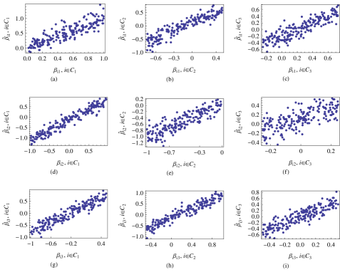
Figure 1: Data were generated based on parameters $\beta_{iv}$’s chosen uniformly in different intervals, $k=3$, $|C_{1}|=190$, $|C_{2}|=193$, $|C_{3}|=197$. The estimated versus the original parameters $\beta_{iv}$’s are shown for $i\in C_{u}$ $(u,v=1,\dots,k)$, where $\beta_{i1}\sim{\cal U}[0,1]$ $(i\in C_{1})$, $\beta_{i1}\sim{\cal U}[-0.75,0.5]$ $(i\in C_{2})$, $\beta_{i1}\sim{\cal U}[-0.25,0.75]$ $(i\in C_{3})$, $\beta_{i2}\sim{\cal U}[-1,1]$ $(i\in C_{1})$, $\beta_{i2}\sim{\cal U}[-1,0]$ $(i\in C_{2})$, $\beta_{i2}\sim{\cal U}[-0.25,0.25]$ $(i\in C_{3})$, $\beta_{i3}\sim{\cal U}[-1,0.5]$ $(i\in C_{1})$, $\beta_{i3}\sim{\cal U}[-0.5,1]$ $(i\in C_{2})$, and $\beta_{i3}\sim{\cal U}[-0.5,0.5]$ $(i\in C_{3})$, respectively.

Fig. 2 shows the resulting clusters obtained by applying our algorithm to the B&K fraternity data [50] with $n=58$ vertices, see also http://vlado.fmf.uni-lj.si/pub/networks/data/ucinet/ucidata.htm#bkfrat. The data, collected by Bernard and Killworth, are behavioral frequency counts, based on communication frequencies between students of a college fraternity in Morgantown, West Virginia. We used the binarized version of the symmetric edge-weight matrix. When the data were collected, the 58 occupants had been living together for at least three months, but senior students had been living there for up to three years. We used our normalized modularity based spectral clustering algorithm [4] to find the starting clusters. In the normalized modularity spectrum we found a gap after the third eigenvalue (in decreasing order of their absolute values), therefore we applied the algorithm with $k=4$ clusters. The four groups are likely to consist to persons living together for about the same time period.

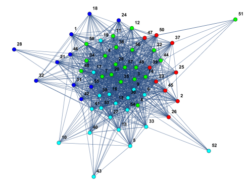
Figure 2: The 4 clusters found by the algorithm in the B&K fraternity data, with 10, 9, 20, and 19 students in the clusters, respectively.

While processing the iteration, occasionally we bumped into the situation when the degree sequence lied on the boundary of the convex polytopes defined in Subsections 2.1 and 2.2. Unfortunately, this can occur when our graph is large but not dense enough. In these situations the iteration did not converge for some coordinates $\beta_{iv}$, but they seemed to tend to $+\infty$ or $-\infty$. Equivalently, the corresponding $\mathbb{b}_{iv}$ for some $i\in C_{u}$ and $v$ tended to $+\infty$ or 0, yielding the situation that member $i\in C_{u}$ had $+\infty$ or 0 affinity towards members of $C_{v}$. Another way, recommended in [8], is to add a small amount to each degree to avoid this situation. However, we did not want to manipulate the original graph, which was too sparse to produce degree sequences in the interior of one or more polytopes.

As for the B&K data, Table 1, Table 2, Table 3, and Table 4 show the $b_{iv}$ parameters for $i\in C_{1},C_{1},C_{3},C_{4}$ and $v=1,2,3,4$. The parameters reflecting attitudes of people of the same group towards each other are usually non-zero finite numbers, whereas there are many zero or infinite parameters in the intercluster relations. These may demonstrate that some groups are quite separated, while some people in some groups show infinite affinity towards persons of some specific groups.

Cluster 1	Cluster 2	Cluster 3	Cluster 4	Label	Degree
0.30083	0	$\infty$	0	1	23
0.70728	$\infty$	$\infty$	0	18	21
1.78066	$\infty$	$\infty$	0	21	23
0.12960	$\infty$	$\infty$	0	24	26
0	0	$\infty$	0	28	6
11.14210	$\infty$	$\infty$	$\infty$	31	39
0.70728	0	$\infty$	0	32	16
0.70728	$\infty$	$\infty$	$\infty$	42	37
11.14210	$\infty$	$\infty$	0	46	29
4.15633	$\infty$	$\infty$	$\infty$	55	41

Table 1: B&K data: the parameters $b_{iv}$, $i\in C_{1}$ and $v=1,2,3,4$; further, label and degree of vertex $i$, $i\in C_{1}$.

Cluster 1	Cluster 2	Cluster 3	Cluster 4	Label	Degree
0	0.27583	$\infty$	0.0154392	2	24
0	15.88360	$\infty$	0.0607916	23	38
0	0.27583	$\infty$	0.0413886	25	25
0	0.10556	$\infty$	0.0103206	26	22
0	2.48471	$\infty$	0.0074528	37	27
0	5.86049	$\infty$	0.0875911	39	38
0	15.88360	$\infty$	0.0592797	45	34
0	0.82970	$\infty$	0.0167808	47	30
0	0.27583	$\infty$	0.0167808	50	28

Table 2: B&K data: the parameters $b_{iv}$, $i\in C_{2}$ and $v=1,2,3,4$; further, label and degree of vertex $i$, $i\in C_{2}$.

Cluster 1	Cluster 2	Cluster 3	Cluster 4	Label	Degree
0	$\infty$	1049.5400	0	3	50
0	0	2.0034	0	4	43
$\infty$	0	1049.5400	0	7	52
0	0	2.0034	0	8	40
0	0	2.0034	0	11	36
0	0	1.2482	0	12	29
0	0	2.0034	0	14	38
0	$\infty$	1049.5400	0	20	50
0	0	1.2482	0	22	34
0	0	8.2779	0	29	46
$\infty$	0	2.0034	0	34	42
0	0	8.2779	0	35	47
0	0	3.5602	0	36	38
0	0	1.2482	0	44	35
0	0	0.4075	0	48	31
0	0	8.2779	0	49	44
0	0	0	0	51	6
0	0	3.5602	0	56	42
0	0	1049.5400	0	57	48
0	0	0.8270	0	58	34

Table 3: B&K data: the parameters $b_{iv}$, $i\in C_{3}$ and $v=1,2,3,4$; further, label and degree of vertex $i$, $i\in C_{3}$.

Cluster 1	Cluster 2	Cluster 3	Cluster 4	Label	Degree
0	10.175	$\infty$	2.73775	5	24
141319.0	282.644	$\infty$	7.91424	6	47
300234.0	282.644	$\infty$	4.50778	9	46
0	4.060	$\infty$	0.24014	10	12
52161.5	35.602	$\infty$	4.50778	13	31
300234.0	63.866	$\infty$	2.73775	15	41
300234.0	121.705	$\infty$	7.91424	16	44
300234.0	35.602	$\infty$	1.74052	17	39
52161.5	35.602	$\infty$	0.42163	19	30
141319.0	63.866	$\infty$	4.50778	27	42
141319.0	2027.000	$\infty$	2.73775	30	42
0	4.060	$\infty$	2.73775	33	27
141319.0	282.644	$\infty$	2.73775	38	38
0	19.762	$\infty$	0.79274	40	21
300234.0	35.602	$\infty$	4.50778	41	40
0	0	$\infty$	0.24014	43	10
0	4.060	$\infty$	0.06535	52	7
52161.5	35.602	$\infty$	4.50778	53	37
141319.0	2027.630	$\infty$	4.50778	54	44

Table 4: B&K data: the parameters $b_{iv}$, $i\in C_{4}$ and $v=1,2,3,4$; further, label and degree of vertex $i$, $i\in C_{4}$.

We also used the network based on the friendships between the users of of the Last.fm music recommendation system [51]. Last.fm is an online service in music based social networking. Each user may have friends inside the Last.fm social network, and so, they form a timestamped undirected graph. In 2012, there were 71,000 users and 285,241 edges between them. Actually, we only used the 15-core of this graph. With spectral clustering tools we found three underlying clusters, see Fig. 3.

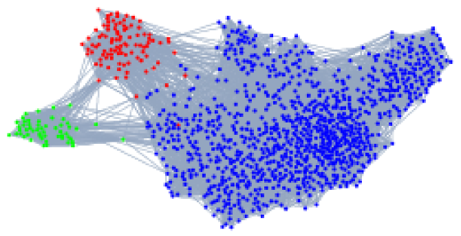
Figure 3: The 3 clusters found by the algorithm in the network of the Last.fm users with 1012, 97, and 53 users in the clusters, respectively.

Fragments of the estimated parameter values are shown in Table 5, Table 6, and Table 7. Here there are some zero affinities, but there are no infinite affinities at all.

Cluster 1	Cluster 2	Cluster 3	Label	Degree
3.099330	0.132913	0	1	329
0.267639	0.036161	0	2	45
0.684764	0	0	3	101
1.174000	0	0	4	159
0.623173	0.014063	0.038484	5	95
0.661509	0	0	6	98
0.886161	0	0	7	126
0.700374	0	0	8	103
0.577860	0.013936	0	9	88
0.446335	0	0	10	69

Table 5: Last.fm data: the parameters $b_{iv}$, $i\in C_{1}$ and $v=1,2,3$; further, label and degree of vertex $i$, $i\in C_{1}$ (first 10 users only).

Cluster 1	Cluster 2	Cluster 3	Label	Degree
1.42735	3.398110	0	41	68
0.21067	0.380953	0	226	20
1.16185	0.302281	0	263	21
0.21067	0.566238	0	286	26
1.16185	0.188533	0	296	16
72.75100	0.468577	5.3444	339	108
1.16185	1.446370	0.7962	340	50
0.90754	2.845830	2.3443	342	65
0.66432	1.139340	0.2664	345	42
0.66432	0.932667	372.2770	351	50

Table 6: Last.fm data: the parameters $b_{iv}$, $i\in C_{2}$ and $v=1,2,3$; further, label and degree of vertex $i$, $i\in C_{2}$ (first 10 users only).

Cluster 1	Cluster 2	Cluster 3	Label	Degree
2.18172	0.288845	2.370600	352	43
3.60021	0.288845	2.370600	370	44
0.18727	4.071150	0.868079	379	37
0.18727	0.288845	3.359140	381	44
0	0.116067	0.589030	421	25
20.69780	0.014618	0.589030	597	34
0.18727	0	0.482873	917	22
0	0.538530	1.914140	942	39
0.18727	0	0.788315	953	27
0	0	1.052870	954	29

Table 7: Last.fm data: the parameters $b_{iv}$, $i\in C_{3}$ and $v=1,2,3$; further, label and degree of vertex $i$, $i\in C_{3}$ (first 10 users only).

5 Conclusions

Our model is the heterogeneous version of the stochastic block model, where the subgraphs and bipartite subgraphs obey parametric graph models, within which the connections are mainly determined by the degrees. The EM type algorithm introduced here finds the blocks and estimates the parameters at the same time.

When investigating controllability of large networks, the authors of [52] observe and prove that a system’s controllability is to a great extent encoded by the underlying network’s degree distribution. In our model, this is true only for the building blocks. Possibly, the blocks could be controlled separately, based on the degree sequences of the subgraphs.

Our model is applicable to large inhomogeneous networks, and above finding clusters of the vertices, it also assigns multiscale parameters to them. In social networks, these parameters can be associated with attitudes of persons of one group towards those in the same or another group. The attitudes are, in fact, affinities to make ties.

References

- [1] Clauset,A., Newman,M.E.J., and Moore,C., Finding community structure in very large networks, Physical Review E 70, 066111 (2004).
- [2] Newman,M.E.J. Networks, An Introduction. Oxford University Press (2010).
- [3] Fortunato,S. Community detection in graphs. Phys. Rep. 486, 75–174 (2010).
- [4] Bolla,M., Penalized versions of the Newman–Girvan modularity and their relation to multiway cuts and -means clustering, Physical Review E 84, 016108 (2011).
- [5] Bolla, M., Spectral Clustering and Biclustering. Learning Large Graphs and Contingency Tables. Wiley (2013).
- [6] Rao,C.R. Linear Statistical Inference and its Applications. Wiley (1973).
- [7] McLachlan,G.J., The EM Algorithm and Extensions. Wiley (1997).
- [8] Chatterjee,S., Diaconis,P. and Sly, A., Random graphs with a given degree sequence, Ann. Statist. 21, 1400-1435 (2010).
- [9] Csiszár,V., Hussami,P., Komlós,J., Móri,T.F., Rejtő,L. and Tusnády,G., When the degree sequence is a sufficient statistic, Acta Math. Hung. 134, 45-53 (2011).
- [10] Rinaldo,A., Petrovic,S. and Fienberg,S.E., Maximum likelihood estimation in the -model, Ann. Statist. 41, 1085-1110 (2013).
- [11] Holland,P.W., Laskey,K.B. and Leinhardt,S., Stochastic blockmodels: some first steps, Social Networks 5, 109-137 (1983).
- [12] Rohe,K., Chatterjee,S. and Yu,B., Spectral clustering and the high-dimensional stochastic blockmodel, Ann. Statist. 39 (4), 1878–1915 (2011).
- [13] Karrer,B. and Newman,M.E.J., Stochastic blockmodels and community structure in networks, Phys. Rev. E 83, 016107 (2011).
- [14] Choi,D.S,, Wolfe,P.J. and Airoldi,E.M., Stochastic blockmodels with growing number of classes, Biometrika 99 (2), 273–284 (2012).
- [15] Fishkind,D.E., Sussman,D.L., Tang,M., Vogelstein,J.T. and Priebe,C.E., Consistent adjacency-spectral partitioning for the stochastic block model when the model parameters are unknown, Siam J. Matrix Anal. Appl. 34 (1), 23-39 (2013).
- [16] Rasch,G.,Studies in Mathematical Psychology: I. Probabilistic Models for Some Intelligence and Attainment Tests. Nielsen and Lydiche, Oxford, UK (1960).
- [17] Rasch,G., On general laws and the meaning of measurement in psychology. In Proc. of the Fourth Berkeley Symp. on Math. Statist. and Probab., pp. 321-333, University of California Press (1961).
- [18] Dempster,A.P., Laird,N.M. and Rubin,D.B., Maximum likelihood from incomplete data via the EM algorithm, J. R. Statist. Soc. B 39, 1-38 (1977).
- [19] Ungar,L.H. and Foster,D.P., A Formal Statistical Approach to Collaborative Filtering. In Proc. Conference on Automatical Learning and Discovery (CONALD 98) (1998).
- [20] Hofmann,T. and Puzicha,J., Latent class models for collaborative filtering. In Proc. 16th International Joint Congress on Artificial Intelligence (IJCAI 99) (ed. Dean T), Vol. 2, pp. 688-693. Morgan Kaufmann Publications Inc., San Francisco CA (1999).
- [21] Casella,G. and George,E.I., Explaining the Gibbs sampler, The American Statistician 46, 167–174 (1992).
- [22] Metropolis,N., Rosenblut,A., Rosenbluth,M., Teller,A. and Teller,E., Equation of state calculation by fast computing machines, J. Chem. Physics 21, 1087–1092 (1953).
- [23] Holland,P.W. and Leinhardt,S., An exponential family of probability distributions for directed graphs, J. Amer. Statist. Assoc. 76, 33-50 (1981).
- [24] Lauritzen,S.L., Extremal families and systems of sufficient statistics. Lecture Notes in Statistics 49, Springer (1988).
- [25] Daudin,J-J., Picard,F. and Robin,S., A mixture model for random graphs, Statistics and Computing 18, 173-183 (2008).
- [26] Newman,M.E.J., Analysis of weighted networks, Physical Review E 70, 056131 (2004).
- [27] Newman,M.E.J., Community detection and graph partitioning, Europhysics Letters 103, 28003 (2013).
- [28] Newman,M.E.J., Mixing patterns in networks, Physical Review E 67, 026126 (2003).
- [29] Bickel,P.J. and Chen,A., A nonparametric view of network models and Newman-Girvan and other modularities, Proc. Natl. Acad. Sci. USA 106 (50), 21068-21073 (2009).
- [30] Reichardt,J. and Bornholdt,S., Partitioning and modularity of graphs with arbitrary degree distribution, Physical Review E 76, 015102(R) (2007).
- [31] Escolano,F., Hancock,E.R. and Lozano,M.A., Heat diffusion: Thermodynamic depth complexity of networks, Physical Review E 85, 036206 (2012).
- [32] Erdős,P. and Rényi,A., On the evolution of random graphs. Publ. Math. Inst. Hung. Acad. Sci. 5, 17-61 (1960).
- [33] Erdős,P. and Gallai, T., Graphs with given degree of vertices (in Hungarian), Matematikai Lapok 11, 264-274 (1960).
- [34] Mahadev,N.V.R. and Peled,U.N., Threshold graphs and related topics, Ann. Discrete. Math. 56, North-Holland, Amsterdam (1995).
- [35] Stanley, L. P., A zonotope associated with graphical degree sequences. In Applied Geometry and Discrete Mathematics. DIMACS Series in Discrete Mathematics and Theoretical Computer Science 4, pp. 555-570. Amer. Math. Soc., Providence, RI. (1991).
- [36] Hammer,P.L., Peled,U.N. and Sun,X., Difference graphs, Discrete Applied Mathematics 28, 35-44 (1990).
- [37] Barvinok,A., What does a random contingency table look like? preprint, arXiv:0806.3910 [math.CO] (2009).
- [38] Borgs,C., Chayes,J.T., Lovász,L, T.-Sós,V. and Vesztergombi,K., Convergent sequences of dense graphs II: Multiway cuts and statistical physics. Ann. Math. 176, 151-219 (2012).
- [39] Haberman,S.J., Log-linear models and frequency tables with small expected counts, Ann. Statist. 5, 1148-1169 (1977).
- [40] Barvinok,A., Matrices with prescribed row and column sums, preprint, arXiv:1010.5706 [math.CO] (2010).
- [41] Gale,D., A theorem on flows in networks, Pacific J. Math. 7, 1073-1082 (1957).
- [42] Ryser,H.J., Combinatorial properties of matrices of zeros and ones, Canad. J. Math. 9, 371-377 (1957).
- [43] Ford,L.R. and Fulkerson,D.R., Maximal flow through a network, Canad. J. Math. 8, 399-404 (1956).
- [44] Barvinok,A., Hartigan,J.A., An asymptotic formula for the number of nonnegative integer matrices with prescribed row and column sums, preprint, arXiv:0910.2477 [math.CO] (2009).
- [45] Barvinok,A., On the number of matrices and a random matrix with prescribed row and column sums and 0-1 entries, preprint, arXiv:0806.1480 [math.CO] (2009).
- [46] Yan,D., Chen,A. and Jordan,M.I., Cluster forests, Comput. Statist. and Data Anal. 66, 178–192 (2013).
- [47] Hastie,T., Tibshirani,R. and Friedman,J., The Elements of Statistical Learning. Data Mining, Inference, and Prediction. Springer (2001).
- [48] Csiszár,V., Hussami,P., Komlós,J., Móri,T.F., Rejtő,L. and Tusnády,G., Testing goodness of fit of random graph models, Algorithms 5, 629-635 (2012).
- [49] Négyessy,L., Nepusz,T., Zalányi,L. and Bazsó,F., Convergence and divergence are mostly reciprocated properties of the connections in the network of cortical areas, Proc. R. Soc. B: Biological Sciences 275, 2403-2410 (2008).
- [50] Bernard,H.R., Killworth,P.D. and Sayler,L., Informant accuracy in social-network data V. An experimental attempt to predict actual communication from recall data, Social Science Research 11, 30-66 (1982).
- [51] Pálovics, R., Benczúr, A., Kocsis, L., Kiss, T. and Frigó, E., Exploiting temporal influence in online recommendation, In Proc. of RecSys’14, 8th ACM Conference on Recommender Systems pp. 273-280, ACM, New York, NY, USA (2014).
- [52] Liu,Y-Y., Slotine,J-J. and Barabási,A-L., Controllability of complex networks, Nature 473, 167-173 (2011).