Numerical construction of initial data for Einstein’s equations
with static extension to space-like infinity

Abstract

We describe a numerical method to construct Cauchy data extending to space-like infinity based on Corvino’s (2000) gluing method. Adopting the setting of Giulini and Holzegel (2005), we restrict ourselves here to vacuum axisymmetric spacetimes and glue a Schwarzschildean end to Brill-Lindquist data describing two non-rotating black holes. Our numerical implementation is based on pseudo-spectral methods, and we carry out extensive convergence tests to check the validity of our numerical results. We also investigate the dependence of the total ADM mass on the details of the gluing construction.

I Introduction

Many situations of astrophysical interest can be described to good approximation as isolated systems: an asymptotically flat spacetime containing a compact self-gravitating source such as a collapsing star, a black hole binary, etc. A fundamental problem in the numerical solution of the Einstein equations for such systems is the treatment of the far field. Access to the asymptotic region known as conformal infinity Frauendiener (2004) is important for several reasons. Firstly, gravitational radiation is only defined in an unambiguous way at future null infinity. Including this region in the computational domain enables extraction of the gravitational radiation emitted by the source in a straightforward way. This is important for the modelling of astrophysical sources of gravitational radiation. Secondly, many open problems in mathematical relativity such as black hole stability and cosmic censorship are statements about the global structure of spacetime. If numerical studies are to shed light on these questions then access to conformal infinity is indispensable.

The standard approach to numerical relativity is based on the Cauchy formulation of Einstein’s equations. The $t=\mathrm{const}$ slices are truncated at a finite distance from the source, where boundary conditions are imposed. These must ensure that the resulting initial-boundary value problem is well posed, they must be compatible with the constraints that hold on the individual $t=\mathrm{const}$ slices, and ideally they should be absorbing, i.e. the artificial boundary should be transparent to gravitational radiation. Despite much progress in this direction (see Sarbach and Tiglio (2012) for a review article), this approach is necessarily limited because exact absorbing boundary conditions cannot be defined at a finite distance in the full nonlinear theory of general relativity so that linearisation about a given background spacetime is typically assumed. And imperfect boundary conditions can easily destroy relevant features of the solutions such as late-time power-law tails caused by the backscattering of gravitational radiation.

An alternative to evolution on truncated Cauchy slices is evolution on hyperboloidal slices extending to future null infinity $\mathrsfs{I}^{+}$. (Examples of hyperboloidal slices are the slices $\Sigma_{1}$ and $\Sigma_{2}$ in Fig. 1.) In this approach a conformal transformation is applied to the spacetime metric, combined with a compactifying coordinate transformation that maps infinity to a finite location. The conformal boundary of the slices becomes a pure outflow boundary so that no boundary conditions are required there. Hyperboloidal evolution was first advocated in general relativity by Friedrich in the context of his regular conformal field equations Friedrich (1983), a symmetric hyperbolic formulation of the (suitably augmented) Einstein equations that is completely regular up to the conformal boundary. For reviews of the theoretical development as well as numerical implementations based on this system, see e.g. Frauendiener (2004); Husa (2002, 2003). An alternative method is based on a straightforward ADM Arnowitt et al. (1962) split of the conformally transformed Einstein equations on hyperboloidal surfaces of constant mean curvature Moncrief and Rinne (2009). The resulting equations are formally singular at $\mathrsfs{I}^{+}$ but can nevertheless be evaluated there in terms of regular conformal data. Based on this system, stable numerical evolutions of a gravitationally perturbed Schwarzschild black hole in axisymmetry were achieved Rinne (2010); later matter fields were also included Rinne and Moncrief (2013); Rinne (2014). Further proposals for hyperboloidal evolution systems that, as far as we know, have not been implemented numerically yet can be found in Zenginoğlu (2008); Bardeen et al. (2011).

The hyperboloidal surfaces are only partial (in our case, future) Cauchy surfaces. The problem remains how to evolve entire spacetimes from Cauchy data extending to space-like infinity. The main difficulty here is that part of the Cauchy data—namely some of the components of the Weyl tensor—are singular at space-like infinity if the ADM mass is not zero Friedrich (1988). In Friedrich (1998) Friedrich proposed a way to render these Cauchy data regular while guaranteeing the regularity of the conformal field equations at space-like infinity. The basic ingredient of this approach is the blowing up of space-like infinity $i^{0}$ to a cylinder $I=[-1,1]\times\mathbb{S}^{2}$ that serves as a link of finite length (along the time direction) between past $\mathrsfs{I}^{-}$ and future $\mathrsfs{I}^{+}$ null infinity. The 2-spheres $I^{\pm}=I\cap\mathrsfs{I}^{\pm}$ where the cylinder meets future and past null infinity are called critical sets. The equations that propagate the data from $\mathrsfs{I}^{-}$ to $\mathrsfs{I}^{+}$ along the cylinder acquire an extremely simple form in Friedrich’s representation that makes them ideal for numerical implementation, see Beyer et al. (2012); Doulis and Frauendiener (2013); Beyer et al. (2014a, b); Frauendiener and Hennig (2014) for some recent numerical work. On the cylinder all the spatial derivatives drop out. Therefore, the cylinder is a total characteristic of the system and hence no boundary conditions are required there. However, this intrinsic system of propagation equations degenerates at the critical sets $I^{\pm}$ and develops logarithmic singularities there that are expected to travel along null infinity and spoil its smoothness. In Friedrich’s approach this generic singular behaviour is successfully reproduced. Its appearance has been made explicit and related to the structure of the initial data. In other words, there is a possibility that by choosing appropriately the initial data the occurrence of non-smooth features in the solutions at null infinity can be avoided. A possible solution proposed already in Friedrich (1998) is to prescribe initial data that respect a set of regularity conditions involving the Cotton tensor. However it turned out Valiente Kroon (2004) that these conditions are not sufficient to prevent the occurrence of the logarithmic singularities in higher order expansions of the solutions of the intrinsic system of propagation equations. In Valiente Kroon (2004) Valiente Kroon proposed a new regularity condition in the form of the following conjecture:

Conjecture.

If an initial data set which is time symmetric and conformally flat in a neighbourhood of infinity yields a development with a smooth null infinity, then the initial data is in fact Schwarzschildean in that neighbourhood.

Recently, the results in Valiente Kroon (2010, 2012) have pointed in favour of the conjecture, but there is still work to be done in order to fully prove it. What has been shown is that the solution is smooth at the critical sets if and only if the initial data is exactly Schwarzschildean in a neighbourhood of infinity. It remains to be proved that the development of the solution along null infinity is smooth if and only if it is smooth at the critical sets. If true, the conjecture unveils the special role that static data play in the smooth development of Cauchy data extending to space-like infinity.

One might object that initial data that are static in a neighbourhood of space-like infinity are overly restrictive. However, a powerful result by Corvino Corvino (2000) suggests that this is not the case. He showed that any given asymptotically flat and conformally flat initial data can be truncated and glued along an annulus to a Schwarzschild metric in the exterior, provided the radius of the gluing annulus is sufficiently large and the mass of the exterior Schwarzschild metric is chosen appropriately. There are otherwise no additional restrictions on the metric in the interior, in particular non-static spacetimes including gravitational radiation are allowed. The method has been generalised to stationary rotating ends described by the Kerr metric, and a cosmological constant has been included Corvino and Schoen (2006); Chruściel and Pollack (2008); Chruściel and Delay (2009); Cortier (2013).

Corvino’s result can be used for the evolution problem as follows (see also Chruściel and Delay (2002)). Since his initial data are Schwarzschild in a neighbourhood of space-like infinity $i^{0}$ on the initial Cauchy slice $\Sigma_{0}$ (see Fig. 1), the future development of these initial data will also be Schwarzschild in a neighbourhood of $i^{0}$ (the shaded region in Fig. 1). By placing an artificial timelike boundary in this region, the data on $\Sigma_{0}$ can be evolved to the future for some time using standard Cauchy evolution with exact boundary conditions taken from the known Schwarzschild solution. From this evolution, data on a hypersurface $\Sigma_{1}$ are obtained, e.g. a hypersurface of constant mean curvature. Outside the artificial boundary, the solution on $\Sigma_{1}$ is known analytically (Schwarzschild), so we obtain data on a complete hyperboloidal surface. These can then be taken as initial data for a hyperboloidal evolution code. For the problem studied in the present paper (vacuum axisymmetric spacetimes), the code developed in Rinne (2010) can in principle be used.

Figure 1: Penrose diagram illustrating the use of our initial data for the evolution problem. The data on the Cauchy surface $\Sigma_{0}$ are glued to a Schwarzschild end (shaded region) and evolved to the surface $\Sigma_{1}$ using Cauchy evolution with a finite boundary (dashed line) in the Schwarzschild region. Given the known Schwarzschild solution, the data on $\Sigma_{1}$ can be completed to a hyperboloidal surface reaching $\mathrsfs{I}^{+}$. This then serves as initial data for a hyperboloidal evolution code.

The present paper deals with the first step of this proposal, namely the construction of initial data based on Corvino’s gluing method. It should be stressed that the proof of Corvino’s theorem is not explicit, i.e. it does not provide us with a prescription for how to actually construct the glued initial data. One of the aims of this paper is to compute such data numerically, at least in a simple setting. We assume here that spacetime is vacuum and axisymmetric. Corvino’s method under these assumptions was first studied analytically by Giulini and Holzegel Giulini and Holzegel (2005). An important achievement of this paper was to turn Corvino’s idea into an explicit PDE problem that can, in principle at least, be solved to obtain the glued data. The 3-metric at a moment of time symmetry in a vacuum axisymmetric spacetime can be written in the form of a Brill wave Brill (1959). This comprises both the Schwarzschild solution in isotropic coordinates and, by superposition, Brill-Lindquist data Brill and Lindquist (1963) for an axisymmetric configuration of two non-rotating black holes (not in equilibrium). Giulini and Holzegel took the metric in the interior to be Brill-Lindquist and glued it to a Schwarzschild metric in the exterior using a general Brill wave metric on the gluing annulus. They were mainly interested in the question whether the ADM mass (i.e., the mass of the exterior Schwarzschild solution) can be smaller than the sum of the two Brill-Lindquist black hole masses, as they expected that this would reduce the (generally unwanted) gravitational radiation introduced in the gluing region. They claimed that this can be done at least to first order in the inverse gluing radius. Using numerical methods we are able to study the solution also for smaller gluing radii.

This paper is organised as follows. In Sec. II we describe the details of the gluing construction and derive the equations to be solved. A novel ingredient is an integrability condition that fixes the relation between the masses of the Brill-Lindquist black holes and the exterior Schwarzschild solution (Sec. II.4). Sec. III is devoted to the numerical implementation. We describe the pseudo-spectral method we use (Sec. III.1) and test the code with an artificial exact solution (Sec. III.2) before turning to the actual gluing problem in Sec. III.3. Detailed convergence tests are carried out. Finally, we investigate how the total ADM mass depends on the details of the gluing procedure (Sec. III.4). We conclude with a discussion of our results and an outlook on future work in Sec. IV.

II The gluing construction

Following the line of thought in Giulini and Holzegel (2005), we set up here the mathematical framework on which our numerical study of the gluing construction in the subsequent section will be based. We will also derive an integrability condition that unveils the dependence of the ADM mass on the details of the gluing construction.

II.1 Basic ingredients

Fig. 2 encapsulates the basic features of the construction proposed in Giulini and Holzegel (2005): the interior spacetime consists of Brill-Lindquist data, the exterior spacetime extending to space-like infinity is Schwarzschild, and the transition between the two data sets takes place along a gluing annulus which is equipped with a Brill wave metric. The gluing annulus extends from $r_{\mathrm{int}}$ to $r_{\mathrm{ext}}$.

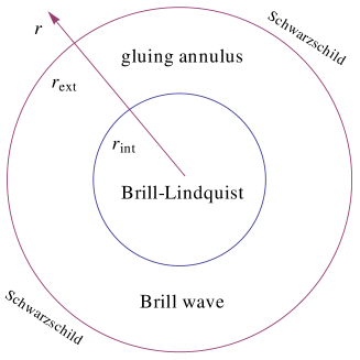
Figure 2: Graphical two-dimensional representation of the gluing construction we are going to consider in the following. A Schwarzschildean end will be glued to Brill-Lindquist data representing two non-rotating black holes in the interior along a transition region equipped with a Brill wave metric.

More specifically, in the interior ($r\leq r_{\mathrm{int}}$) we consider axisymmetric vacuum Brill-Lindquist data Brill and Lindquist (1963) describing two black holes at a moment of time symmetry,

$$g_{\textrm{\tiny B-L}}=\left(1+\frac{m_{1}}{2|\vec{r}-\vec{c}_{1}|}+\frac{m_{2}}{2|\vec{r}-\vec{c}_{2}|}\right)^{4}\delta,$$ (II.1)

where $\delta=dr^{2}+r^{2}(d\theta^{2}+\sin^{2}\theta\,d\phi^{2})$ denotes the three-dimensional Euclidean line element in spherical polar coordinates, and $m_{k}$ and $\vec{c}_{k}$, with $k=1,2$, are the bare masses and coordinate centres of the two black holes, respectively. In order to simplify our formulation, we will assume in the following that the two black holes are of equal mass, i.e. $m_{1}=m_{2}=m$, and that they lie symmetrically to the origin on the z-axis, i.e. $\vec{c}_{1}=-\vec{c}_{2}=\vec{c}=(0,0,\frac{d}{2})$, see Fig. 3. With these choices the line element (II.1) reduces to

$$g_{\textrm{\tiny B-L}}=\left(1+\frac{m}{2|\vec{r}-\vec{c}|}+\frac{m}{2|\vec{r}+\vec{c}|}\right)^{4}\delta.$$ (II.2)

Notice that the above line element is written in conformally flat form, a feature that will play a key role in the subsequent development of the gluing construction. It can be readily confirmed that the ADM mass of the Brill-Lindquist data (II.2) is equal to $2m$.

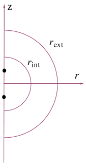
Figure 3: The Brill-Lindquist data. We consider two black holes of equal mass positioned symmetrically to the origin on the z-axis. The two black holes are at a moment of time symmetry, i.e. they do not carry any spin and they are momentarily at rest relative to each other.

In the present work we will consider only Brill-Lindquist data where the horizons of the two black holes do not intersect. Also all cases where a third outer horizon Brill and Lindquist (1963), enclosing both black holes, forms—which appears when the black holes are very close to each other—would not be considered here. As shown in Brill and Lindquist (1963) both the above requirements are satisfied when the mass-to-distance ratio satisfies the inequality $m/d\lesssim 0.64$. In this setting, the radius of the event horizon of each of the black holes is given by the formula Brill and Lindquist (1963)

$$r_{\mathrm{hor}}=\frac{m}{2+\frac{m}{d}}.$$

Therefore in the following, in order to keep the gluing annulus away from any possible horizons of the Brill-Lindquist data, the gluing radius $r_{\mathrm{int}}$ will be chosen in such a way that the inequality $r_{\mathrm{int}}>d/2+r_{\mathrm{hor}}$ is always satisfied.

We intend to glue a Schwarzschildean end to the Brill-Lindquist data (II.2) residing in the interior of our construction. Thus, in the exterior ($r\geq r_{\mathrm{ext}}$) of the gluing annulus we consider the usual spherically symmetric Schwarzschild data, which when expressed in isotropic coordinates can be written in the following conformally flat form,

$$g_{\textrm{\tiny Schw}}=\left(1+\frac{M}{2|\vec{r}|}\right)^{4}\delta.$$ (II.3)

By construction, the mass $M$ is identical with the ADM mass of the entire glued initial data.

The above two data sets (II.2) and (II.3) will be glued together using a Brill wave. This choice follows naturally from the axisymmetric nature of the Brill-Lindquist data considered in the interior of the construction. Brill waves Brill (1959) are the most general axisymmetric vacuum spacetimes with hypersurface-orthogonal Killing vector. In spherical coordinates, the spatial metric at a moment of time symmetry is given by the Weyl-type line element

$$g_{\textrm{\tiny Brill}}=\psi^{4}\left(e^{2\,q}(dr^{2}+r^{2}d\theta^{2})+r^{2}\sin^{2}\theta\,d\phi^{2}\right).$$ (II.4)

The function $q(r,\theta)$ will be the unknown of our construction. It must satisfy the boundary conditions

$$q=0\qquad\mathrm{for}\,\,\,\theta=0,\,\pi,$$ (II.5)

$$\frac{\partial q}{\partial\theta}=0\qquad\mathrm{for}\,\,\,\theta=0,\,\pi.$$

The latter condition follows from the fact that $q$ is an even function of $\theta$. To justify the former, one has first to write the metric (II.4) in Cartesian coordinates and inspect the behaviour of its metric coefficients on the z-axis; then the vanishing of $q$ along the z-axis follows as a necessary regularity condition that guarantees the absence of any conical singularities on it Rinne and Stewart (2005). The conformal factor $\psi(r,\theta)$ introduced above must be positive definite everywhere and must satisfy the asymptotic conditions $\displaystyle\lim_{r\to\infty}\psi=1$ at space-like infinity.

In summary, we want to construct a spacetime that is Brill-Lindquist (II.2) in the interior $r\leq r_{\mathrm{int}}$, is of general Brill wave form (II.4) on the intermediate gluing annulus $r_{\mathrm{int}}\leq r\leq r_{\mathrm{ext}}$, and is Schwarzschild (II.3) in the exterior $r\geq r_{\mathrm{ext}}$. In addition, all the transitions between the different regions must be smooth.

II.2 The recipe

The novelty of Giulini’s and Holzegel’s construction lies in the way they incorporated Corvino’s original idea Corvino (2000) solely into the definition of the conformal factor $\psi$, i.e. the metric on the entire three-dimensional time-symmetric slice is given by the Brill wave metric (II.4) with

$$\psi=\left(1+\frac{m}{2|\vec{r}-\vec{c}|}+\frac{m}{2|\vec{r}+\vec{c}|}\right)\beta(r,\theta)+(1-\beta(r,\theta))\left(1+\frac{M}{2|\vec{r}|}\right).$$ (II.6)

Here $\beta(r,\theta)$ is the so-called gluing function, which apart of being smooth has the following properties:

$$\beta(r,\theta)=\left\{\begin{array}[]{l l}1,&\quad r\leq r_{\mathrm{int}},\\ 0,&\quad r\geq r_{\mathrm{ext}},\end{array}\right.$$ (II.7)

and all its $r$-derivatives must vanish at $r=r_{\mathrm{int}}$ and $r=r_{\mathrm{ext}}$. The precise form of the gluing function that is going to be used in the present work is left for Sec. III.1.

Let us see now how the gluing construction described in Sec. II.1 can be realised by the choice (II.6) of the conformal factor. Notice that the first and second term in (II.6) are of Brill-Lindquist and Schwarzschildean character, respectively. In the interior $r\leq r_{\mathrm{int}}$ the gluing function equals unity, $\beta=1$, therefore the second term in (II.6) vanishes. Thus, the conformal factor $\psi$ consists now only of its Brill-Lindquist part; inserting it into the Brill wave metric (II.4) and enforcing $q$ to vanish in the interior region, the Brill wave coincides exactly with the Brill-Lindquist data (II.2). In a similar manner in the exterior $r\geq r_{\mathrm{ext}}$ only the Schwarzschildean part of $\psi$ survives, as $\beta=0$ there. Again inserting the resulting conformal factor in (II.4) and setting $q=0$ also in the exterior region, the Brill wave (II.4) coincides with the Schwarzschildean data (II.3). In the intermediate region $r_{\mathrm{int}}\leq r\leq r_{\mathrm{ext}}$ the conformal factor $\psi$, and consequently the function $q$ in (II.4), have a more complicated form.

The function $q(r,\theta)$ in the gluing region will be determined by Einstein’s equations. In addition to the boundary conditions (II.5) on the z-axis, smoothness requires that $q$ and all its radial derivatives vanish at the boundaries of the gluing annulus:

$$q=0\quad\mathrm{and}\quad\frac{\partial^{n}\!q}{\partial r^{n}}=0\qquad\mathrm{at}\quad r=r_{\mathrm{int}},r_{\mathrm{ext}},$$ (II.8)

for all $n\in\mathbb{N}$. The boundary conditions that $q$ must satisfy are summarised in Fig. 4.

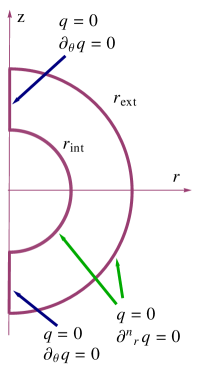
Figure 4: The boundary conditions. The thick lines indicate the loci where boundary conditions on the function $q$ must be imposed. On the z-axis the conditions (II.5) related to the axisymmetry of our construction must be satisfied while on the boundaries of the gluing annulus the conditions (II.8) must be implemented.

II.3 Mathematical fomulation

Having set up our gluing scheme in the previous sections, we now move on to Einstein’s equations. On the initial slice these reduce to the momentum and Hamiltonian constraints. The former is identically satisfied as our data are time-symmetric, so we are left only with the Hamiltonian constraint, which in the time-symmetric case reduces to the vanishing of the Ricci scalar of the Brill wave metric (II.4), i.e.

$$R({g}_{\textrm{\tiny Brill}})=0.$$

Expanding the Ricci scalar in the above expression, the Hamiltonian constraint results in an inhomogeneous Poisson equation of the form

$${}^{(2)}\Delta q = -4\,\frac{{}^{(3)}\Delta\psi}{\psi}\quad:\Leftrightarrow$$

$$\frac{\partial^{2}q}{\partial r^{2}}+\frac{1}{r^{2}}\frac{\partial^{2}q}{\partial\theta^{2}}+\frac{1}{r}\frac{\partial q}{\partial r} = -\frac{4}{\psi}\left(\frac{\partial^{2}\psi}{\partial r^{2}}+\frac{1}{r^{2}}\frac{\partial^{2}\psi}{\partial\theta^{2}}+\frac{2}{r}\frac{\partial\psi}{\partial r}+\frac{\cot\theta}{r^{2}}\frac{\partial\psi}{\partial\theta}\right)=:f.$$ (II.9)

According to our construction in Sec. II.2, the right-hand side of the above elliptic equation is specified by the form of $\psi$ that is defined by (II.6) and (II.7). Since this is fixed a priori, we will consider the right-hand side of (II.3) as an inhomogeneity and denote it by $f$. It should be noted that (II.3) reduces to a homogeneous Poisson equation outside the gluing annulus as the constancy of $\beta$ enforces $f$ to vanish there. Summarising, our goal in the following will be to numerically solve the second-order linear PDE (II.3) for $q(r,\theta)$ subject to the boundary conditions (II.5) and (II.8).

II.4 Integrability condition

At first sight it might seem that the choice of the two mass parameters $m$ and $M$ in the conformal factor (II.6) is unconstrained. If this were true then nothing would prevent us from gluing a Minkowskian end to the Brill-Lindquist data in the interior! This would obviously violate the positive mass theorem Schoen and Yau (1979). In fact Einstein’s equations constrain the choice of the masses. One way to see this is by employing the machinery developed by Brill Brill (1959) in order to prove that the ADM mass of time-symmetric, axisymmetric, vacuum gravitational waves is positive definite. It turns out that in our setting this result can be used as a condition to determine the relation between the masses involved in our construction.

Following Brill’s arguments in Brill (1959), we repeat here his original derivation adjusted to the details of our construction. Our starting point is the Poisson equation (II.3) expressed in cylindrical coordinates $(\rho,\phi,z)$:

$$\frac{\partial^{2}q}{\partial\rho^{2}}+\frac{\partial^{2}q}{\partial z^{2}}+\frac{4}{\psi}\left(\frac{\partial^{2}\psi}{\partial\rho^{2}}+\frac{\partial^{2}\psi}{\partial z^{2}}+\frac{1}{\rho}\frac{\partial\psi}{\partial\rho}\right)=0,$$

which when expressed in terms of the three-dimensional flat Laplace operator $\nabla^{2}=\rho^{-1}\partial_{\rho}+\partial^{2}_{\rho}+\rho^{-2}\partial^{2}_{\phi}+\partial^{2}_{z}$ in cylindrical coordinates takes the form

$$4\,\frac{\nabla^{2}\psi}{\psi}+\nabla^{2}q-\frac{1}{\rho}\frac{\partial q}{\partial\rho}=0.$$

Integrating over the interior $V$ of a large sphere $\Sigma$ of radius $R$ centred at the origin, one gets

$$4\int_{V}\left[\nabla\cdot\left(\frac{\nabla\psi}{\psi}\right)+\left(\frac{\nabla\psi}{\psi}\right)^{2}\right]dV+\int_{V}\nabla^{2}q\,dV-\int_{V}\frac{1}{\rho}\frac{\partial q}{\partial\rho}\,dV=0,$$ (II.10)

where the gradient and the divergence in cylindrical coordinates read $\nabla=(\partial_{\rho},\rho^{-1}\partial_{\phi},\partial_{z})$ and $\nabla\cdot=(\rho^{-1}+\partial_{\rho},\rho^{-1}\partial_{\phi},\partial_{z})\cdot\,$, respectively. The integration of the last term reads

$$\int_{V}\frac{1}{\rho}\frac{\partial q}{\partial\rho}\,\rho\,d\rho\,d\phi\,dz=2\,\pi\int_{-R}^{R}\left[q\left(\sqrt{R^{2}-z^{2}},z\right)-q(0,z)\right]dz=-2\,\pi\int^{\pi}_{0}q(R,\theta)\,R\,\sin\theta\,d\theta,$$

where in the last step we used the first of the boundary conditions (II.5) and expressed the remaining term in spherical coordinates. In the rest of the proof, the first two integrals in (II.10) will also be expressed in spherical coordinates. Inserting the result of the above integration into (II.10) and re-expressing the first and third term through the divergence theorem, one arrives at

$$8\,\pi\int^{\pi}_{0}\left.\frac{1}{\psi}\frac{\partial\psi}{\partial r}\right|_{r=R}R^{2}\sin\theta\,d\theta+4\int_{V}\left(\frac{\nabla\psi}{\psi}\right)^{2}dV+2\,\pi\int^{\pi}_{0}\left[\left.\frac{\partial q}{\partial r}\right|_{r=R}R^{2}+q(R,\theta)\,R\right]\sin\theta\,d\theta=0.$$ (II.11)

In the limit $R\rightarrow\infty$ the last term of the above expression vanishes because $q=0$ for $r>r_{\textrm{ext}}$. In addition, according to (II.6), the conformal factor in the limit $R\rightarrow\infty$ behaves like $1+\frac{M}{2\,R}$; thus the first term of the expession above reads

$$8\,\pi\int^{\pi}_{0}\left.\frac{1}{\psi}\frac{\partial\psi}{\partial r}\right|_{r=R}R^{2}\sin\theta\,d\theta=8\,\pi\int^{\pi}_{0}\frac{-\frac{M}{2\,R^{2}}}{1+\frac{M}{2\,R}}R^{2}\sin\theta\,d\theta\overset{R\rightarrow\infty}{=}-8\,\pi\,M.$$

Taking into account the last two results, (II.11) in the limit $R\rightarrow\infty$ reduces to

$$-2\,\pi\,M+\int_{V}\left(\frac{\nabla\psi}{\psi}\right)^{2}dV=0.$$

Finally, expanding the integrand and integrating over $\phi$ one arrives at Brill’s original expression for the ADM mass,

$$M=\int^{\pi}_{0}\int^{\infty}_{0}\left[\left(\frac{1}{\psi}\frac{\partial\psi}{\partial r}\right)^{2}+\left(\frac{1}{r\,\psi}\frac{\partial\psi}{\partial\theta}\right)^{2}\right]r^{2}\sin\theta\,dr\,d\theta,$$ (II.12)

which is obviously positive definite. It is interesting that this expression for the ADM mass only depends on the conformal factor. Recall that the ADM mass $M$ of our construction appears in the definition of the conformal factor (II.6) and consequently is also present in the integrand above. Based on this observation one can use (II.12) as an integrability condition for the ADM mass, namely the integral on the right-hand side of (II.12) for a specific choice of $M$ must return the same value for the ADM mass.

III Numerical implementation of the gluing construction

In this section our numerical implementation of the gluing construction described in the previous section and some first numerical results are presented.

III.1 Setting up the numerical scheme

We choose to solve the Poisson equation (II.3) numerically using pseudo-spectral methods. Accordingly, the unknown function $q(r,\theta)$ is approximated by a truncated series of suitable specific polynomials. We choose to expand the $r$-dependence of $q$ in Chebyshev polynomials $T_{k}$ and the $\theta$-dependence in Fourier-cosine series for reasons (in addition to the ones presented in Bonazzola et al. (1999)) that will soon become apparent.

Our two-dimensional physical domain is given by $(r,\theta)\in[r_{\mathrm{int}},r_{\mathrm{ext}}]\times[0,\pi]$. While the range of the angular coordinate $\theta$ is in accordance with the expansion in Fourier-cosine series, the range of the radial coordinate $r$ is not, as the Chebyshev polynomials are defined on the interval $[-1,1]$. In order to map the original $r$-domain to $[-1,1]$, we use the mapping

$$x\mapsto r(x):=\frac{1}{2}(r_{\mathrm{ext}}-r_{\mathrm{int}})\,x+\frac{1}{2}(r_{\mathrm{ext}}+r_{\mathrm{int}}),$$

where $x$ takes values in the interval $x\in[-1,1]$. Therefore, from now on, we have to think of the expressions (II.6), (II.7) and (II.3) as expressed in terms of this new linearly transformed radial coordinate $x$. Therefore, in the following our two-dimensional computational domain will be $D=[-1,1]\times[0,\pi]$. A finite representation of $D$ is obtained by the introduction of equidistant collocation points in the $\theta$-direction and of non-equidistant Gauss-Lobatto collocation points in the radial direction, namely

$$\theta_{i}=\frac{i\,\pi}{L}\qquad\mathrm{and}\qquad x_{j}=-\cos\left(\frac{j\,\pi}{K}\right)\qquad\mathrm{with}\qquad i=0,\ldots,L\quad\mathrm{and}\quad j=0,\ldots,K,$$

where $K$ and $L$ is the number of collocation points along the radial and $\theta$-direction, respectively.

Let us now turn to the boundary conditions (II.5) and (II.8). In fact this is by far the most involved part of our numerical implementation. In order to satisfy (II.8) we make the following ansatz:

$$q(x,\theta)=B(x)\,\hat{q}(x,\theta),$$ (III.1)

where $\hat{q}$ is an arbitrary function of its arguments and $B(x)$ is a function of “bump” character on the gluing annulus, i.e. $B(x)$ and all its $x$-derivatives vanish on the boundaries of the gluing annulus. An example of a “bump” function with the above properties looks like

$$B(x)=\mathrm{sech}\left(\frac{b_{1}}{x-1}+\frac{b_{2}}{x+1}\right),$$ (III.2)

where $b_{1},b_{2}$ are constants. The convergence of our numerical solutions crucially depends on the choice of these constants. It has been observed that the convergence properties of the produced numerical solutions are optimal when the constants $b_{1},b_{2}$ take values $b_{1},b_{2}<1$. In the following the choice $b_{1}=b_{2}=10^{-2}$ will always be used. The second boundary condition in (II.5) is satisfied if one expands the newly introduced function $\hat{q}(x,\theta)$ in the way described in the first paragraph of this section, namely

$$\hat{q}(x,\theta)=\sum^{K}_{k=0}{\sum^{L}_{l=0}{a_{kl}\,T_{k}(x)\,\cos(l\,\theta)}},$$ (III.3)

where $K,L$ are as above and the constants $a_{kl}$ are the expansion coefficients of our series. In order to satisfy the remaining boundary condition, i.e. the first of (II.5), one can use the freedom inherent in the choice of the gluing function (II.7). Recall that the gluing function, apart from the specific conditions that it has to satisfy on the boundaries of the gluing annulus, can be freely specified otherwise. A possible ansatz is

$$\beta(x,\theta)=\alpha(x)+\hat{\alpha}(x)B(x)\sin^{2}\theta,$$ (III.4)

where

$$\alpha(x)=\frac{1}{2}\left(1+\tanh\left(\frac{1}{x-1}+\frac{1}{x+1}\right)\right),$$

$B(x)$ is given by (III.2) and $\hat{\alpha}(x)$ is a so far arbitrary function that we choose in order to enforce the condition $q=0$ on the z-axis. Notice that the function $\alpha(x)$ takes the values $1$ and $0$ on the internal $x=-1$ and external $x=1$ boundary of the gluing annulus, respectively, and all its spatial derivatives vanish there; thus, it satisfies all the criteria of (II.7). The inclusion of the “bump” function $B(x)$ in the ansatz (III.4) guarantees that, independently of the choice of $\hat{\alpha}(x)$, the second term in (III.4) and all its derivatives vanish identically on the boundaries. Therefore, the form of $\hat{\alpha}(x)$ influences the shape of $\beta(x,\theta)$ only in the interior of the gluing annulus. (It is noteworthy that with a $\theta$-independent ansatz, e.g. of the form $\beta(x)=\alpha(x)+\hat{\alpha}(x)B(x)$, it was not possible to satisfy the first boundary condition in (II.5) and at the same time have a convergent numerical solution.) Now, as the roots of the map

$$\hat{\alpha}(x)\mapsto q(x,\theta\in\{0,\pi\})$$ (III.5)

are $(K+1)$-dimensional vectors (recall $K$ refers to the number of radial collocation points), we have to use a multidimensional secant (quasi-Newton) method to find them. (We chose to use a secant instead of a Newton method as the former is computationally less costly and faster.) The most effective and efficient method of this kind has proven Press et al. (2007) to be Broyden’s method Broyden (1965). Given an initial guess for $\hat{\alpha}(x)$, Broyden’s method tries to find iteratively the form of $\hat{\alpha}(x)$ that leads to a solution of (II.3) satisfying the first boundary condition in (II.5) to a given accuracy (here to the order of $\sim 10^{-14}$). In the following the roots of (III.5) will be computed numerically using the implementation of Broyden’s method in the optimize sub-package of Python’s SciPy library.

Summarising, by assuming that $q$ in (III.1) is a multiple of a “bump” function $B$, the vanishing of $q$ and all its $x$-derivatives at $x=\pm 1$ is guaranteed. The expansion of $\hat{q}$ as a Fourier-cosine series sets $\partial_{\theta}\hat{q}$ to zero on the $z$-axis; consequently $\partial_{\theta}q$ also vanishes there as $\partial_{\theta}q=B\,\partial_{\theta}\hat{q}$. Finally, an appropriate choice of the function $\hat{\alpha}(x)$ in the ansatz (III.4) can make $q$ vanish on the $z$-axis.

So far we have assumed that the mass parameter $M$ appearing in the conformal factor (II.6) is given. However, this parameter has to agree with the integral expression (II.12) for the ADM mass, which contains the conformal factor—hence $M$ is only given implicitly. We start by choosing an initial value for $M$ and solve for $q$ and $\hat{\alpha}$ using the iterative procedure described above. Knowing $\hat{\alpha}$ and thus the gluing function $\beta$, we can compute the conformal factor (II.6) and evaluate the value $M_{I}$ of the integral for the ADM mass (II.12). Then we vary $M$ until a value satisfying $M=M_{I}$ is found, repeating the above procedure at each step. This will be illustrated in Sec. III.4.

The code has been written from scratch in Python.

III.2 Testing the code with an exact solution

Before we start using our code to study numerically the Poisson equation (II.3), we will carry out—as one should always do—some numerical tests to check the performance of our code. For this a family of exact solutions will be used. The exact solutions will be computed in the following way. First, we choose a $q$ and compute analytically the outcome of the left-hand side of (II.3), then we equate the resulting expession with the inhomogeneity $f$. Now, having at hand the expression for $f$, one can solve numerically (II.3) for $q$ and compare the outcome with the exact expression of $q$ chosen originally. This procedure will give us hints about the accuracy and the convergence properties of the code.

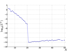
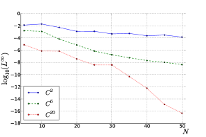
Figure 5: Convergence against the exact solutions (III.6). Shown is the $L^{\infty}$ norm of the error as a function of the number of grid points $N$. (a) The exact solution $q$ is smooth, i.e. infinitely differentiable $\mathcal{C}^{\infty}$. The characteristic “step” behaviour of polynomial functions is clearly visible. (b) The exact solution $q$ is of finite differentiability. As expected the higher the differentiability of the solution, the faster the convergence.

As exact solutions we will use the following family of functions,

$$q(x,\theta)=x^{\kappa/3}\left(x-1\right)^{10}\left(x+1\right)^{10}\sin(6\,\theta)B(x)\sin\theta,$$ (III.6)

where $\kappa$ is a non-negative integer and $B$ is the “bump” function (III.2). The main reason for choosing the above family of solutions is that it allows us to control, through the choice of $\kappa$, the differentiability, and consequently the smoothness, at $x=0$. Obviously, if $\kappa$ is zero or a multiple of three, then the function $\hat{q}$ corresponding to (III.6) is a polynomial and thus infinitely differentiable $\mathcal{C}^{\infty}$. For any other value of $\kappa$, (III.6) is finitely differentiable $\mathcal{C}^{j}$. In the following, we will assume that $\kappa$ takes the values $\kappa=0,7,19,61$ and as a consequence the solution (III.6) will be $\mathcal{C}^{\infty},\mathcal{C}^{2},\mathcal{C}^{6},\mathcal{C}^{20}$ at $x=0$, respectively. Our goal of doing all this is not only to show that the numerical solutions converge to the exact ones, but also to observe the expected relation, see e.g. Trefethen (2000), between the convergence of the numerical solutions and the smoothness of the exact solution, i.e. the smoother the solution (III.6), the faster the convergence of the code.

Our findings are presented in Fig. 5. Both graphs therein depict the $\log_{10}$ of the absolute value of the maximum error (in other worlds the $L^{\infty}$ norm) between the numerical and the corresponding exact solution for different numbers of grid points $N$, where here we have chosen $K=L=:N$. Fig. 5 illustrates the case of smooth functions ($\kappa=0$). Here one observes the typical “step” behaviour of the convergence plots corresponding to polynomial functions Trefethen (2000); this is because the Chebyshev polynomials form a complete basis for the polynomials, so that (III.6) is represented exactly for $N>20$ (the error settles down to numerical roundoff $\sim 10^{-14}$). On the other hand, Fig. 5 shows the case of finitely differentiable functions. It can be easily seen that in all the cases considered the numerical solutions converge to the exact ones, but with different speed. A detailed inspection of the individual plots shows that, as expected, the speed of convergence is faster the smoother is our solution Trefethen (2000).

III.3 Numerical realisation of the gluing construction

III.3.1 Results

The results of the previous section constitute strong evidence that our code can reproduce successfully the exact solutions (III.6), and its convergence behaviour is as expected. Thus, we are confident enough to proceed further in the numerical study of the gluing construction and look for general solutions of (II.3).

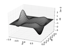
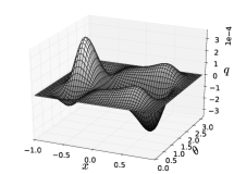
Figure 6: Numerical solutions of (II.3). The function $q$ is plotted on the grid $D=[-1,1]\times[0,\pi]$ for the choice $m=2$, $d=10$, $r_{\mathrm{ext}}=2\,r_{\mathrm{int}}$, and gluing radii (a) $r_{\mathrm{int}}=50$, (b) $r_{\mathrm{int}}=100$, (c) $r_{\mathrm{int}}=500$. The corresponding ADM masses are (a) $M=4.001084$, (b) $M=4.00002725$ and (c) $M=4.0000000095$, see Fig. 11. Notice the order of magnitude of the solutions; as expected, it decreases with the distance of the gluing annulus from the origin. The numerical resolution used here is $K=L=25$ collocation points.

In order to do so, one has first to choose appropriately the free parameters entering the definition of the conformal factor (II.6) and then to compute the inhomogeneity $f$ by evaluating the right-hand side of (II.3). Recall that according to its definition, the conformal factor depends on the mass $m$ of the individual Brill-Lindquist black holes, their mutual distance $d$, the mass $M$ of the exterior Schwarzschild region, the location of the gluing annulus $r_{\mathrm{int}},r_{\mathrm{ext}}$, and the form of the gluing function (II.7). In the following, the ansatz (III.4) will be used for the gluing function and the form of $\hat{\alpha}(x)$ entering its definition will be computed in accordance with the discussion of Sec. III.1. Except for a couple of conditions that constrain their choice, the above parameters can be freely chosen. The first condition follows from the fact that the gluing annulus has to be placed away from any horizons of the Brill-Lindquist data; for this the inequality $r_{\mathrm{int}}>d/2+r_{\mathrm{hor}}$ must always be satisfied—see Sec. II.1 for the details. The second condition constrains the relation of the masses $m$ and $M$, as discussed in Sec. II.4.

Fig. 6 shows several numerical solutions of the system (II.3), (II.5), (II.8) for the following choice of the free parameters: $m=2$, $d=10$, $r_{\mathrm{ext}}=2\,r_{\mathrm{int}}$, and the ADM mass $M$ has been chosen such that the integrability condition (II.12) is satisfied (see Fig. 11). Starting from Fig. 6, the distance of the gluing annulus from the origin has been gradually increased from $r_{\mathrm{int}}=50$ to $r_{\mathrm{int}}=500$. As expected, the further away one places the gluing annulus, the smaller the numerically computed values of $q$ become. This behaviour follows naturally from the fact that the Brill-Lindquist data (II.2) look more and more like Schwarzschild data the further away one goes from the origin; consequently, the Brill wave—essentially the function $q$—does not have to do “a lot of work” to glue the two sets of data together. Similar behaviour is observed when the distance of the annulus from the origin is kept fixed but its width is gradually increased. Now, the magnitude of $q$ gradually decreases as it has “more and more space” to perform the gluing between the two data sets.

The results of Fig. 6 are the first evidence that the gluing constructions proposed in Corvino (2000); Giulini and Holzegel (2005) can be realised numerically. Whereas the analysis of Corvino (2000); Giulini and Holzegel (2005) applies only to the case when the gluing annulus is placed at large distances, our numerical findings here demonstrate that these results can be extended to smaller gluing radii.

At this point, it is worth checking what happens in the case that the distance between the two black holes is taken to be $d=0$ so that there is only a single black hole of mass $2m$ in the centre. One would expect that as long as the condition $M=2m$ is satisfied, the function $q$ must vanish; for in this setting the Brill-Lindquist data (II.2) are already in Schwarzschild form. It turns out that our code correctly reproduces the trivial solution for arbitrary position of the gluing annulus.

III.3.2 Convergence analysis

Let us turn now to the convergence analysis of our numerical solutions. In contrast to Sec. III.2, here we do not have an exact solution to compare our numerical findings with. Thus, we have to follow a different approach to check the convergence of our numerical solutions. The usual way to proceed in such a situation is to study the decay of the expansion coefficients $a_{kl}$ in (III.3), see Boyd (2001). The expansion coefficients $a_{kl}$ must gradually decay to zero for increasingly large indices in order for the series expansion (III.3) to converge. Once $q$ has been computed numerically, the expansion coefficients can be readily evaluated by inverting (III.3).

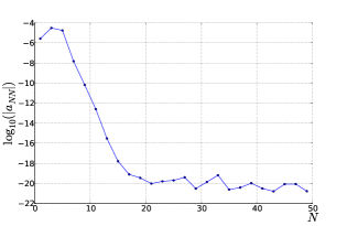
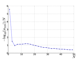
Figure 7: Exponential decay of the expansion coefficients with the number of grid points $N$. (a) The diagonal expansion coefficients for $N<20$ fall off in an almost linear fashion in this logarithmic plot, indicating exponential decay. (b) Testing for exponential decay. The ratio $-\log_{10}(|a_{NN}|)/N$ must asymptote to a non-negative number in the limit $N\rightarrow\infty$.

Fig. 7 depicts the results of our convergence analysis for the numerical solution of Fig. 6. Because of the two-dimensional nature of the series expansion (III.3), one has to choose along which direction to study $a_{kl}$. We chose here to study the convergence behaviour of the diagonal expansion coefficients $a_{NN}$ as they provide a good indication of the overall decay of $a_{kl}$. The fall-off behaviour of $|a_{NN}|$ is depicted in Fig. 7 on a logarithmic scale; the observed approximately linear behaviour for $N<20$ suggests an exponential decay to the roundoff plateau. To make this statement more quantitative, one has to study the ratio $-\log_{10}(|a_{NN}|)/N$ in the limit $N\rightarrow\infty$. Therefore, following Boyd (2001), if the limit

$$\lim_{N\to\infty}\left(\frac{-\log_{10}(|a_{NN}|)}{N}\right)\geq 0$$

is a non-negative number then the expansion coefficients converge to zero exponentially. In Fig. 7 one clearly sees a tendency of the ratio $-\log_{10}(|a_{NN}|)/N$ to asymptote to a small positive number, which is a strong indication of exponential decay.

We will conclude the present section by presenting another indication that the numerical solutions produced in Sec. III.3.1 converge exponentially. In Fig. 8, on a rectangular $N\times N/4$ grid (i.e. $N$ grid points along the radial and $N/4$ along the angular direction), we compare numerical solutions of different resolutions to the one with the highest resolution for the solution of Fig. 6. Specifically, the numerical values of $q$ for each resolution are interpolated onto the same grid and compared with the solution of highest resolution there (here an $100\times 25$ grid). Finally, the $L^{2}$-norm of the absolute value of the error for each resolution has been plotted on a logarithmic scale, see Fig. 8. The curve falls off in an approximately linear fashion.

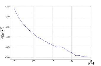
Figure 8: Convergence with respect to the numerical solution of highest resolution. The logarithm of the error falls off roughly linearly with the number of grid points $N/4$ along the angular direction.

III.4 Behaviour of the ADM mass

We will now investigate the dependence of the ADM mass on the details of the gluing construction. Namely, we examine if it is possible to choose the free parameters entering the definition of the conformal factor (II.6) in such a way that the ADM mass $M$ can take values different from the sum of the two Brill-Lindquist black holes, i.e. $M\neq 2\,m$. The case $0<M<2\,m$ corresponds to a reduction of the ADM mass, while the case $M>2\,m$ to an increase. In other words, we explore the possibility of gluing together the spacetimes (II.2) and (II.3) under the assumption that their asymptotic behaviour at space-like infinity (when considered separately) is different.

As already mentioned in Sec. II.4, the integrability condition (II.12) can be used to study the dependence of the ADM mass on the details of the gluing construction. After choosing the free parameters entering (II.6) and computing the form of $\hat{\alpha}(x)$ entering the definition of the gluing function (III.4) in the way described in Sec. III.1, the integral (II.12) will be computed numerically using the integrate sub-package of the Python SciPy library. The value of the integral computed in this way will be denoted by $M_{I}$ in contrast to the parameter $M$ chosen originally.

Depending on the choice of the free parameters, the right-hand side of (II.12), i.e. $M_{I}$, can take on values that do not necessarily agree with $M$. In this case the integrability condition would be violated, $\Delta M=M_{I}-M\neq 0$. Here, we will only be interested in the case that $M_{I}=M$ holds, corresponding to a true physical solution.

To exemplify the use of the condition (II.12), we will use as a test case the scenario that the distance $d$ between the black holes in the interior is taken to be zero. In this setting, there is a single black hole of mass $2m$ in the centre to which we attempt to glue a Schwarzschildean end of ADM mass $M$. Fig. 9 depicts how the integrability condition constrains the possible choice of the masses $m,M$. Therein, we have plotted the difference $\Delta M=M_{I}-M$ between the integral (II.12) and the originally chosen value $M$ of the ADM mass as a function of the ADM mass $M$. For the choice $m=2$, $r_{\mathrm{int}}=100$ and $r_{\mathrm{ext}}=2\,r_{\mathrm{int}}$ the curve crosses the $M$-axis, i.e. the integrability condition $\Delta M=0$ is satisfied, in two distinct points: $M_{1}=4$ and $M_{2}\approx 4.095$. The first crossing corresponds to the case that the two Schwarzschildean data sets are identical $M_{1}=2m$. Obviously, in this case the Brill wave responsible for the gluing must be trivial, i.e. $q=0$ as it was confirmed at the end of Sec. III.3.1. The second crossing now corresponds to a setting where the two Schwarzschildean data sets we attempt to glue together are different $M_{2}\neq 2m$; the Brill wave performing the gluing is now non-trivial, i.e. $q\neq 0$. Therefore, the results of Fig. 9 entail that for the class of gluing functions (III.4) we consider, the integrability condition allows us to glue a Schwarzschildean end of ADM mass $M_{1}=4$ or $M_{2}\approx 4.095$ to the single black hole of mass $2m$ residing in the centre. Any other combination of the masses would lead to non-physical solutions that violate Einstein’s equations.

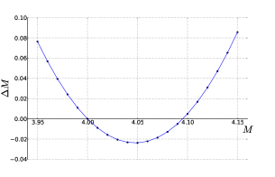
Figure 9: The integrability condition in action. Shown is the difference $\Delta M=M_{I}-M$ between the integral (II.12) and the originally chosen value $M$ of the ADM mass. As a test case we assume that the data in the interior and exterior of the gluing annulus are Schwarzschildean, i.e. $d=0$. In this setting, the integrability condition locks the choice of the masses to $M_{1}=4\pm 3.736\times 10^{-11}$ or $M_{2}\approx 4.095$. The former corresponds to the case of gluing together two identical $M_{1}=2m$ Schwarzschildean data sets, the latter to the case that the ADM mass of the data in the exterior is larger than the corresponding mass in the interior $M_{2}>2m$.

Let us return now to the behaviour of the ADM mass for general separations $d$ of the two black holes. In order to check if the integrability condition allows for a reduction (increase) of the ADM mass, we will fix $m$ and study the dependence of the difference $\Delta M=M_{I}-M$ on the ADM mass $M$ for different locations of the gluing annulus. If the violation $\Delta M$ of the integrability condition has different signs for two different values of the ADM mass $M$, then according to the intermediate value theorem $\Delta M$ must vanish somewhere in between these two values of $M$. In Fig. 10, the free parameters were chosen to be $m=2$, $d=10$, $r_{\mathrm{ext}}=2\,r_{\mathrm{int}}$, and the gluing annulus has been placed at $r_{\mathrm{int}}=30$ or $100$. The curve for $r_{\mathrm{int}}=100$ crosses the $M$-axis twice for values $M>2m=4$—for the first crossing this will be clarified in Fig. 10—and hence the ADM is increased. For $r_{\mathrm{int}}=30$ the curve does not cross the $M$-axis, indicating that, for the choice of the free parameters we are using, there are no physically admissible solutions of (II.3). The same behaviour is observed for any choice of $r_{\mathrm{int}}\lesssim 40$, implying that the gluing is not possible for these positions of the annulus. On the other hand, for $r_{\mathrm{int}}\gtrsim 40$ the curve always crosses the $M$-axis twice for $M>4$.

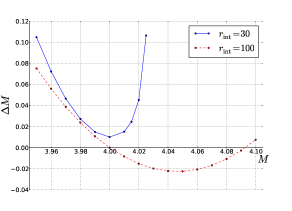
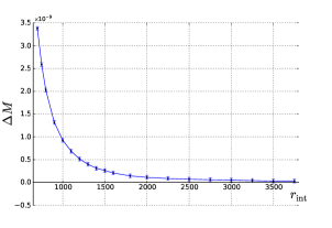
Figure 10: Behaviour of the ADM mass. (a) The difference $\Delta M$ between the integral value $M_{I}$ of the ADM mass and the given parameter $M$ is plotted as a function of the ADM mass $M$ for different values of the gluing radius $r_{\mathrm{int}}$. When placing the gluing annulus at $r_{\mathrm{int}}=100$ the condition $\Delta M=0$ is satisfied for $M>4$; thus only increase of the ADM mass is possible. Notice that in the case $r_{\mathrm{int}}=30$ the integrability condition cannot be satisfied for any value of $M$; thus (II.3) does not have any physically admissible solutions. (b) The difference $\Delta M$ as a function of the gluing radius $r_{\mathrm{int}}$ for the choice $M=4$. Whenever $\Delta M>0$ the ADM mass increases. The error bars indicate the numerical error.

To clarify this point further, we have plotted in Fig. 10 for the first crossing the difference $\Delta M$ as a function of the gluing radius $r_{\mathrm{int}}$ for fixed $M=4$. (Here, we will concentrate on the behaviour of the ADM mass at the first crossing because if the first crossing happens for $M_{1}>4$ then certainly the second crossing will happen for $M_{2}>M_{1}>4$.) Based on the results of Fig. 10, one can safely conclude that close to the first crossing $\Delta M$ decreases with $M$; therefore, if $\Delta M$ is positive for $M=4$ then an appropriate increase of $M$ will cause $\Delta M$ to vanish—a setting that leads to an increase of the ADM mass of the glued solution. Fig. 10 provides strong evidence that the ADM mass is increased for any position of the gluing annulus (no matter how far out). For gluing radii larger than $r_{\mathrm{int}}=3500$ the violation $\Delta M$ becomes of the same order of magnitude of the numerical error, i.e. $10^{-11}$, which indicates that it is not possible to draw any decisive conclusions about the behaviour of $\Delta M$ there. However, one expects that $\Delta M$ asymptotes to zero from positive values as the gluing annulus is progressively placed further out: in the limiting case that the gluing is performed at infinity, where the two spacetimes become indistinguishable, the Brill wave becomes trivial and $\Delta M$ vanishes.

Let us look a little more closely into the details of the increase of the ADM mass and try to determine it quantitatively. As already indicated by Fig. 10, the increase is larger for smaller gluing radii $r_{\mathrm{int}}$. In Fig. 11 the actual increase of the ADM mass, $M_{I}-2m$, for different locations of the gluing annulus is presented. Notice that the amount of increase, $M_{I}-2m$, reduces extremely fast to zero with increasing gluing radius: increasing the gluing radius from $r_{\mathrm{int}}=50$ to $100$ results in a decrease of $M_{I}-2m$ by two orders of magnitude.

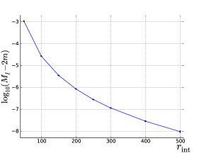
Figure 11: Increase of the ADM mass as a function of the gluing radius. For $r_{\mathrm{int}}=50$ and $r_{\mathrm{int}}=100$ the increase amounts to $(1.084\pm 0.0003)\times 10^{-3}$ and $(2.725\pm 0.007)\times 10^{-5}$, respectively. By just doubling the gluing radius the increase of the ADM mass decreases by a factor of 40.

It was mentioned above that the increase of the ADM mass can be attributed to the presence of the Brill wave responsible for the gluing. To further clarify this point, we will consider the integrability condition (II.12) in the form

$$M(\chi)=\int^{\pi}_{0}\int^{\chi}_{0}\left[\left(\frac{1}{\psi}\frac{\partial\psi}{\partial r}\right)^{2}+\left(\frac{1}{r\,\psi}\frac{\partial\psi}{\partial\theta}\right)^{2}\right]r^{2}\sin\theta\,dr\,d\theta,$$ (III.7)

where the upper limit of the radial integration takes values in the interval $\chi\in[0,\infty)$. Obviously $M(0)=0$ and in the limit $M(\chi\rightarrow\infty)=M$ one obtains the total ADM mass of the gluing construction. In the case we have only pure Brill-Lindquist data, i.e. there is no gluing, we have $M_{B-L}(\chi\rightarrow\infty)=2\,m$. According to Fig. 11, $M(\infty)-M_{B-L}(\infty)$ is always positive. In the interior $\chi\in[0,r_{\mathrm{int}}]$, the difference $M(\chi)-M_{B-L}(\chi)$ must be zero as in both cases the data there are Brill-Lindquist. Therefore, there must be a point where $M(\chi)$ departs from $M_{B-L}(\chi)$ to positive values. This behaviour is studied in Fig. 12, where the difference $M(\chi)-M_{B-L}(\chi)$ has been plotted as a function of $\chi$ for the choice $m=2$, $M=4.001084$, $d=10$, $r_{\mathrm{int}}=50$, $r_{\mathrm{ext}}=2\,r_{\mathrm{int}}$ corresponding to the numerical solution of Fig. 6. It is apparent that the main contribution to the increase of the ADM mass comes from the region where the gluing takes place, i.e. $\chi\in[50,100]$; in the interior $\chi<50$ the difference $M(\chi)-M_{B-L}(\chi)$ vanishes as expected; in the exterior $\chi>100$ the difference $M(\chi)-M_{B-L}(\chi)$ asymptotes to the positive value given in Fig. 11. Thus, it seems that indeed the Brill wave is responsible for the increase of the ADM mass.

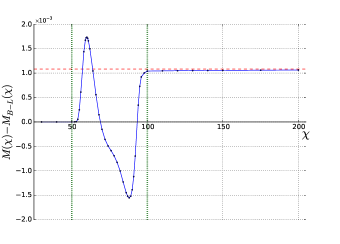
Figure 12: Contribution of the Brill wave to the increase of the ADM mass. The integrability condition (III.7) has been used to plot the difference $M(\chi)-M_{B-L}(\chi)$ between glued and pure Brill-Lindquist data as a function of the radial coordinate $\chi$ for the choice $m=2$, $M=4.001084$, $d=10$, $r_{\mathrm{int}}=50$, $r_{\mathrm{ext}}=2\,r_{\mathrm{int}}$. The pair of vertical dotted (green) lines denote the span of the gluing annulus. The horizontal dashed (red) line indicates the positive value $M(\infty)-M_{B-L}(\infty)=0.001084$ given in Fig. 11 corresponding to the amount of increase of the ADM mass. It can be clearly seen that the main contribution to this increase comes from inside the gluing annulus.

We conclude with a brief discussion on the possibility of reducing the ADM mass. Our extensive numerical study of the solution space of (II.3), corresponding to the specific choice (III.4) of the gluing function, points in the direction that reduction of the ADM mass is not possible. As already pointed out in Fig. 12, the key point in reducing the ADM mass is to find a way to reduce the contribution of the Brill wave to it. In Fig. 10 we tried to do so by increasing the gluing radius (i.e. placing the gluing annulus further and further out); it was shown that reduction of the ADM mass cannot be achieved in this way. Other possible ways to “weaken” the Brill wave are widening the gluing annulus and decreasing the distance between the black holes. In Fig. 13 the behaviour of the ADM mass is studied in a setup where the black holes are placed very close to each other and the gluing annulus is extremely wide. Specifically, we choose the mass of each one of the black holes to be $m=2$ and the distance between them $d=3.2$. For this choice the mass-to-distance ratio $m/d=0.625$ just respects the condition $m/d\lesssim 0.64$, see Sec. II.1, which prevents the appearance of a third outer horizon enclosing both black holes. The horizon of each black hole is $r_{\mathrm{hor}}=0.761905$ and thus the gluing radius must always satisfy $r_{\mathrm{int}}\gtrsim 2.4$. We fix the mass parameter to be $M=4$. In this setting, we plot in Fig. 13 the difference $\Delta M$ between the integral value $M_{I}$ of the ADM mass and the given parameter $M$ as a function of the position of the inner boundary $r_{\mathrm{int}}$ of the gluing annulus for three different locations of the outer boundary: $r_{\mathrm{ext}}=100,300$ and $500$. (Recall that reduction or increase of the ADM mass is possible when $\Delta M<0$ or $\Delta M>0$, respectively.) Our findings indicate that reduction is not possible even in this extreme scenario. Although the increase of the ADM mass is smaller the further out we place the outer boundary, the behaviour of all curves remains qualitatively the same: the difference $\Delta M$ remains always positive and an initial decrease of $\Delta M$ is followed by an increase while moving the inner boundary towards the outer boundary. The latter behaviour follows naturally from the fact that moving the inner boundary towards the outer one narrows the gluing annulus, leaving less and less space for the Brill wave to perform the gluing and thus increasing its contribution to the ADM mass.

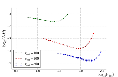
Figure 13: Behaviour of the ADM mass in an extreme scenario. The difference $\Delta M$ between the integral value $M_{I}$ of the ADM mass and the given parameter $M$ for the configuration $m=2$, $M=4$, $d=3.2$, and three different locations of the outer boundary $r_{\mathrm{ext}}=100,300,500$ is presented as a function of the inner gluing radius $r_{\mathrm{int}}$. (For reasons of presentation we use a logarithmic scale on both axes.) Reduction of the ADM mass is not possible as $\Delta M$ is always positive.

IV Discussion

The purpose of this paper was to demonstrate for the first time how Corvino’s gluing construction Corvino (2000) can be implemented numerically in order to compute nontrivial Cauchy data that are Schwarzschild in a neighbourhood of space-like infinity.

Our numerical implementation is based on the analytical work by Giulini and Holzegel Giulini and Holzegel (2005), who applied Corvino’s method to axisymmetric vacuum spacetimes. In their setting, spacetime is Brill-Lindquist (II.2) out to some radius, is described by a general Brill wave (II.4) along an intermediate gluing region, and is Schwarzschild (II.3) outside this region. Einstein’s equations determine the equation to be solved numerically, namely the second-order linear PDE (II.3) subject to the boundary conditions (II.5) and (II.8). In order to obtain physically meaningful solutions, one has to constrain the choice of the two mass parameters $m$ and $M$ appearing in the definition of the conformal factor. It turns out that Einstein’s equations imply an integrability condition (II.12) that can be used for this purpose. In addition, we make sure that the gluing region lies outside of any black hole horizons.

To solve numerically the elliptic equation describing the gluing construction, we chose to use pseudo-spectral methods. An extensive convergence analysis, both for an artificial exact solution (Sec. III.2) and for the actual gluing problem (Sec. III.3.2), demonstrates the accuracy and convergence of our numerical solutions. Our results confirm the behaviour that one would intuitively expect: the numerically computed values of $q$ decrease with increasing distance of the gluing annulus from the origin and increasing width, see Fig. 6.

Giulini and Holzegel Giulini and Holzegel (2005) wondered whether it is possible to choose the gluing parameters in such a way that the ADM mass $M$ is smaller than $2m$, the sum of the two Brill-Lindquist black hole masses. By reducing the ADM mass, one might hope to reduce the amount of gravitational radiation that is known to be contained in the Brill-Lindquist data Sperhake (2007). Our findings in Sec. III.4 suggest that the presence of the Brill wave in the gluing region generically tends to increase the ADM mass. We have not been able to reduce the ADM mass even in the rather special setup where the black holes are placed extremely close to each other and the gluing region extends from close to the black hole horizons to a large distance, see Fig. 13. It should be stressed though that there is a lot of freedom in the choice of the gluing function $\beta$. Here we tried only the ansatz (III.4). It could be that there exist gluing functions that lead to a reduction of the ADM mass, even though we think this is unlikely. So our results do not necessarily contradict the asymptotic analysis of Giulini and Holzegel (2005).

We remark that there are other proposals for constructing Cauchy data extending to space-like infinity that are not based on Corvino’s gluing method. For example, Avila Avila (2011) considered initial data that are only asymptotically static up to a given order at space-like infinity. It would be interesting to implement this approach numerically as well. Evolving such data to future null infinity is likely to be more complicated than in our approach, where spacetime is known a priori in a whole neighbourhood of space-like infinity.

Our ultimate goal is to compute an entire spacetime from the Cauchy data constructed using the methods described in this paper. As a first step, we will evolve our data to a first hyperboloidal surface reaching future null infinity; this can then be used as initial data for a hyperboloidal evolution code based on either the regular conformal field equations or the alternative approaches described in Sec. I.

V Acknowledgments

We are grateful to Carla Cederbaum, Helmut Friedrich, Domenico Giulini, Gustav Holzegel and Martín Reiris for helpful discussions. This research is supported by grant RI 2246/2 from the German Research Foundation (DFG) and a Heisenberg Fellowship to O.R.

References

- Frauendiener (2004) J. Frauendiener, “Conformal infinity,” Living Rev. Relativity 7, 1 (2004).
- Sarbach and Tiglio (2012) O. Sarbach and M. Tiglio, “Continuum and discrete initial-boundary value problems and Einstein’s field equations,” Living Rev. Relativity 15, 9 (2012).
- Friedrich (1983) H. Friedrich, “Cauchy problems for the conformal vacuum field equations in general relativity,” Commun. Math. Phys. 91, 445–472 (1983).
- Husa (2002) S. Husa, “Problems and successes in the numerical approach to the conformal field equations,” Lect. Notes Phys. 604, 239–260 (2002), grqc/0204043 .
- Husa (2003) S. Husa, “Numerical relativity with the conformal field equations,” Lect. Notes Phys. 617, 159–192 (2003), grqc/0204057 .
- Arnowitt et al. (1962) R. Arnowitt, S. Deser, and C. W. Misner, “The dynamics of general relativity,” in Gravitation: an introduction to current research, edited by L. Witten (Wiley, New York, 1962) Chap. 7.
- Moncrief and Rinne (2009) V. Moncrief and O. Rinne, “Regularity of the Einstein equations at future null infinity,” Class. Quantum Grav. 26, 125010 (2009), 0811.4109 .
- Rinne (2010) O. Rinne, “An axisymmetric evolution code for the Einstein equations on hyperboloidal slices,” Class. Quantum Grav. 27, 035014 (2010), 0910.0139 .
- Rinne and Moncrief (2013) O. Rinne and V. Moncrief, “Hyperboloidal Einstein-matter evolution and tails for scalar and Yang-Mills fields,” Class. Quantum Grav. 30, 095009 (2013), 1301.6174 .
- Rinne (2014) O. Rinne, “Formation and decay of Einstein-Yang-Mills black holes,” to appear in Phys. Rev. D (2014), 1409.6173 .
- Zenginoğlu (2008) A. Zenginoğlu, “Hyperbolodial evolution with the Einstein equations,” Class. Quantum Grav. 25, 195025 (2008), 0808.0810 .
- Bardeen et al. (2011) J. M. Bardeen, O. Sarbach, and L. T. Buchman, “Tetrad formalism for numerical relativity on conformally compactified constant mean curvature hypersurfaces,” Phys. Rev. D 83, 104045 (2011), 1101.5479 .
- Friedrich (1988) H. Friedrich, “On static and radiative space-times,” Commun. Math. Phys. 119, 51–73 (1988).
- Friedrich (1998) H. Friedrich, “Gravitational fields near space-like and null infinity,” J. Geom. Phys. 24, 83–163 (1998).
- Beyer et al. (2012) F. Beyer, G. Doulis, J. Frauendiener, and B. Whale, “Numerical space-times near space-like and null infinity. The spin-2 system on Minkowski space,” Class. Quantum Grav. 29, 245013 (2012), 1207.5854 .
- Doulis and Frauendiener (2013) G. Doulis and J. Frauendiener, “The second order spin-2 system in flat space near space-like and null-infinity,” Gen. Relativ. Gravit. 454, 1365–1385 (2013), 1301.4286 .
- Beyer et al. (2014a) F. Beyer, G. Doulis, J. Frauendiener, and B. Whale, “Linearized gravitational waves near space-like and null infinity,” Springer Proc. Math. Stat. 60, 3–17 (2014a), 1302.0043 .
- Beyer et al. (2014b) F. Beyer, G. Doulis, J. Frauendiener, and B. Whale, “The spin-2 equation on Minkowski background,” Springer Proc. Math. Stat. 60, 465–468 (2014b), 1304.6458 .
- Frauendiener and Hennig (2014) J. Frauendiener and J. Hennig, “Fully pseudospectral solution of the conformally invariant wave equation near the cylinder at spacelike infinity,” Class. Quantum Grav. 31, 085010 (2014), 1311.6786 .
- Valiente Kroon (2004) J.-A. Valiente Kroon, “A new class of obstructions to the smoothness of null infinity,” Commun. Math. Phys. 244, 133–156 (2004), grqc/0211024 .
- Valiente Kroon (2010) J.-A. Valiente Kroon, “A rigidity property of asymptotically simple spacetimes arising from conformally flat data,” Commun. Math. Phys. 298, 673–706 (2010), 0906.4714 .
- Valiente Kroon (2012) J.-A. Valiente Kroon, “Asymptotic simplicity and static data,” Ann. Henri Poincaré 13, 363–397 (2012), 1011.6600 .
- Corvino (2000) J. Corvino, “Scalar curvature deformation and a gluing construction for the Einstein constraint equations,” Commun. Math. Phys. 214, 137–189 (2000).
- Corvino and Schoen (2006) J. Corvino and R. M. Schoen, “On the asymptotics for the vacuum Einstein constraint equations,” J. Diff. Geom. 73, 185–217 (2006), grqc/0301071 .
- Chruściel and Pollack (2008) P. T. Chruściel and D. Pollack, “Singular Yamabe metrics and initial data with exactly Kottler-Schwarzschild-de Sitter ends,” Ann. Henri Poincaré 9, 639–654 (2008), 0710.3365 .
- Chruściel and Delay (2009) P. T. Chruściel and E. Delay, “Gluing constructions for asymptotically hyperbolic manifolds with constant scalar curvature,” Comm. Anal. Geom. 17, 343–381 (2009), 0711.1557 .
- Cortier (2013) J. Cortier, “Gluing construction of initial data with Kerr-de Sitter ends,” Ann. Henri Poincaré 14, 1109–1134 (2013), 1202.3688 .
- Chruściel and Delay (2002) P. T. Chruściel and E. Delay, “Existence of non-trivial, vacuum, asymptotically simple spacetimes,” Class. Quantum Grav. 19, L71–L79 (2002), grqc/0203053 .
- Giulini and Holzegel (2005) D. Giulini and G. Holzegel, “Corvino’s construction using Brill waves,” Preprint (2005), grqc/0508070 .
- Brill (1959) D. R. Brill, “On the positive mass of the Bondi-Weber-Wheeler time-symmetric gravitational waves,” Ann. Phys. 7, 466–483 (1959).
- Brill and Lindquist (1963) D. R. Brill and R. W. Lindquist, “Interaction energy in geometrostatics,” Phys. Rev. 131, 471–476 (1963).
- Rinne and Stewart (2005) O. Rinne and J. M. Stewart, “A strongly hyperbolic and regular reduction of Einstein’s equations for axisymmetric spacetimes,” Class. Quantum Grav. 22, 1143–1166 (2005), grqc/0502037 .
- Schoen and Yau (1979) R. Schoen and S.-T. Yau, “On the proof of the positive mass conjecture in general relativity,” Commun. Math. Phys. 65, 45–76 (1979).
- Bonazzola et al. (1999) S. Bonazzola, E. Gourgoulhon, and J.-A. Marck, “Spectral methods in general relativistic astrophysics,” J. Comput. Appl. Math 109, 433–473 (1999), grqc/9811089 .
- Press et al. (2007) W. H. Press, S. A. Teukolsky, W. T. Vetterling, and B. P. Flannery, Numerical recipes: The art of scientific computing, 3rd ed. (Cambridge university press, 2007).
- Broyden (1965) C. G. Broyden, “A class of methods for solving nonlinear simultaneous equations,” Math. Comp. 19, 577–593 (1965).
- Trefethen (2000) L. N. Trefethen, Spectral methods in MATLAB, 1st ed. (SIAM, 2000).
- Boyd (2001) J. P. Boyd, Chebyshev and Fourier spectral methods, 2nd ed. (Dover publications, 2001).
- Sperhake (2007) U. Sperhake, “Binary black-hole evolutions of excision and puncture data,” Phys. Rev. D 76, 104015 (2007), grqc/0606079 .
- Avila (2011) G. A. Avila, Asymptotic staticity and tensor decompositions with fast decay conditions, Ph.D. thesis, University of Potsdam (2011).