Breather-like solitons extracted from the Peregrine rogue wave

Abstract

Based on the Peregrine solution (PS) of the nonlinear Schrödinger (NLS) equation, the evolution of rational fraction pulses surrounded by zero background is investigated. These pulses display the behavior of a breather-like solitons. We study the generation and evolution of such solitons extracted, by means of the spectral-filtering method, from the PS in the model of the optical fiber with realistic values of coefficients accounting for the anomalous dispersion, Kerr nonlinearity, and higher-order effects. The results demonstrate that the breathing solitons stably propagate in the fibers. Their robustness against small random perturbations applied to the initial background is demonstrated too.

I Introduction

The Peregrine solution (PS), which was discovered more than 30 years ago Peregrine , is one of the soliton solutions of the nonlinear Schrödinger (NLS) equation existing on top of a finite continuous-wave (CW) background. Recently, the PS has drawn renewed attention due to its unique localization dynamics Zakharov ; Shrira ; Khawaja ; Chen . Particularly, it has been extensively studied as a prototype of the oceanic rogue waves, and is called, in this context, the Peregrine rogue wave. Actually, the PS is a limit case of other NLS solitons existing on the finite background, viz., the Kuznetsov-Ma soliton, localized in the transverse dimension Kuznetsov ; Ma , and of the Akhmediev breather, which is localized in the longitudinal dimension Akhmediev . It was found that a small perturbation on top of the CW background may grow into the full Peregrine rogue wave, pumped by the modulation (Benjamin-Feir) instability of the background Kharif ; Slunyaev ; Ruban ; Andonowati . Experimental observations concerning the formation and dynamics of the Peregrine rogue wave in diverse physical media, such as optical fibers, water-wave tanks, and plasmas, have been recently reported Kibler ; Chabchoub ; Bailung . Splitting of the Peregrine rogue wave under non-ideal initial conditions, which exhibits its instability, has been demonstrated too Hammani .

Another species of solutions of equations of the NLS type is represented by breathers (breathing solitons), which periodically oscillate in the course of the evolution. A well-known example is the dispersion-managed soliton, in which the periodic dilatation and compression is induced by the alternating map of the anomalous and normal group velocity dispersion Smith ; Nakazawa ; Yu ; Shapiro ; book ; DM-review . Generally, breathers exist in systems with periodically modulated parameters, such as dispersion, gain/loss and nonlinearity coefficients, which can be used for amplification and compression of solitons book ; Serkin1 ; Serkin2 ; RuiyuHao . The concept of breathing solitons is also known in the theory of nonlinear dissipative systems governed by generic complex Ginzburg-Landau equations, in which self-sustained breathers are supported by the balance between the dispersion and nonlinearity, concomitant with equilibrium between gain and loss. Well-known examples of such dissipative breathers are provided, chiefly, by laser cavities and similarly organized systems featuring the combination of amplification and dissipation Petv ; PhysicaD ; Deissler ; lasers ; Tlidi ; Akhmediev1 ; AK ; Rosanov ; Vladimir ; Song . Breathers are known too in models of nonlocal nonlinear media Bezuhanov ; Zhanghuafeng ; Strinic ; Aleksic ; Petrovic . Furthermore, breather-type solitons have been predicted in a variety of other physically relevant settings, including, inter alia, discrete PRL86:2353 and continuous PRL95:050403 models of Bose-Einstein condensates, third-harmonic generation in nonlinear optics OC229:391 , reaction-diffusion systems PRE74:066201 , elastic rods with the mechanical nonlinearity represented by a combination of quadratic and cubic terms PSSB249:1386 , and dynamical models of galaxies astro .

In this work, using the spectral-filtering method, we aim to study the generation and propagation of breather-like solitons generated by the Peregrine rogue waves in optical fibers with anomalous dispersion, Kerr nonlinearity and high-order effects. The results help to understand unique properties of the Peregrine rogue waves and design experimental generation of the breathers in optical fibers. In this connection, it may be relevant to mention recent works which demonstrated the generation of multiple solitons, both freely moving ones and arrays in the form of the Newton’s cradle cradle (see also Ref. Lu ), as a result of splitting of a high-order NLS breather under the action of the third-order dispersion, and emission of solitons by Airy waves in the nonlinear fiber Marom .

The paper is organized as follows. In the next Section, we recapitulate the Peregrine solution of the NLS equation. Then we present a rational fraction pulse, and discuss its propagation properties that are similar to those of breathers. In Sec. III, we investigate the generation, propagation, and stability of such oscillating solitons in the nonlinear fiber. Conclusions are summarized in Sec. IV.

II The Peregrine solution for NLS equation and the rational fraction pulse

In the picosecond regime, the dynamics of the optical pulse propagation in optical fibers is governed by the scaled NLS equation in the well-known form Kodama ; Agrawal ,

$$i\frac{\partial q}{\partial z}+\frac{1}{2}\frac{\partial^{2}q}{\partial t^{2}}+|q|^{2}q=0,$$ (1)

where $q=q(z,t)$ is the slowly varying envelope of the electric field, $t=t^{\prime}-z/v_{g}$, $v_{g}$ stands for the group velocity, while $t$ and $z$ represent the retarded temporal coordinate and normalized propagation distance, respectively. The rational PS of the NLS equation is Peregrine

$$q(z,t)=Ae^{iA^{2}Z}\left[1+R\left(Z,T\right)\right],$$ (2)

with

$$R(Z,T)=\frac{-4-i8A^{2}Z}{1+4A^{4}Z^{2}+4A^{2}T^{2}},$$ (3)

and $T=t-t_{0}$, $Z=z-z_{0}$, where $t_{0}$, $z_{0}$, and $A$ are arbitrary real constants. Equation (2) demonstrates that the PS is a superposition of a CW solution and a fraction function, in which the nonzero CW background pushes an initial local weak pulse towards nonlinear compression via the modulation instability. The largest compression of the pulse is attained at $z=z_{0}$ ($Z=0$) Hammani , as shown in Figs. 1(a) and 1(c). As a possible application, the maximally compressed pulse can be used to generate high-power pulses, with the help of the spectral-filtering technique Ygy1 ; Ygy2 . This method allows one to eliminate the CW background around the maximally compressed pulse in the temporal domain, therefore the shape of the high-power pulses, obtained by means of the spectral filtering, is chiefly determined by the fraction part of solution (2).

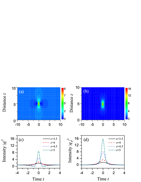
Figure 1: (Color online) The contour plots of (a) the Peregrine rogue wave given by Eq. (2) and (b) the rogue wave with zero CW background given by Eq. (4). The growing intensity distributions at propagation distances $z=3.5$, $z=4$, $z=4.5$, and $z=5$, respectively, are shown in (c) for the Peregrine rogue wave, and in (d) for the rogue wave with zero CW background. The parameters are $A=1$, $z_{0}=5$, and $t_{0}=0$.

Now we turn to the consideration of the rational fraction part of solution (2), taking it as

$$q_{T}(z,t)=Ae^{iA^{2}Z}R\left(Z,T\right).$$ (4)

This expression is not an exact solution for the NLS equation, but it is localized in time and the propagation direction, and is surrounded by zero background, as seen in Fig. 1(b). Thus, for fixed $z$, expression (4) represents a fraction pulse, whose intensity distributions at different distances are shown in Fig. 1(d). Comparing Figs. 1(d) with Fig. 1(c), we concluded that the corresponding intensities of the fraction pulse are larger than those of the PS. Furthermore, it is straightforward to find the peak power, full-width at half-maximum (FWHM), and energy of the rogue wave with zero background

$$P\left(Z\right) \equiv\left|q_{T}\left(z,t_{0}\right)\right|^{2}=\frac{16A^{2}}{1+4A^{4}Z^{2}},$$

$$W\left(Z\right) =\frac{\sqrt{(\sqrt{2}-1)(1+4A^{4}Z^{2})}}{A},$$

$$E\left(Z\right) \equiv\int_{-\infty}^{+\infty}\left|q_{T}\right|^{2}dt=\frac{4A\pi}{\sqrt{1+4A^{4}Z^{2}}},$$ (5)

as functions of propagation distance $z$. Figure 2 shows their evolution along $z$ (recall that $Z=z-z_{0}$). From here, one can see that, at $z\leq z_{0}$, the peak power and energy of the fraction pulse increases with the propagation distance $z$. One can also find that the peak power and energy of this pulse increase with the decrease of the pulse’s width until $z=z_{0}$, and the largest peak power and energy are attained, naturally, at the narrowest pulse width. Small circles in Figs. 2(a-c) correspond to the peak power, width and energy of the growing fraction pulse at $z=3.5$, $4$, $4.5$ and $5$, see Fig. 1(d). Thus, the fraction pulse can be used to generate narrow waveforms with prescribed peak powers and widths.

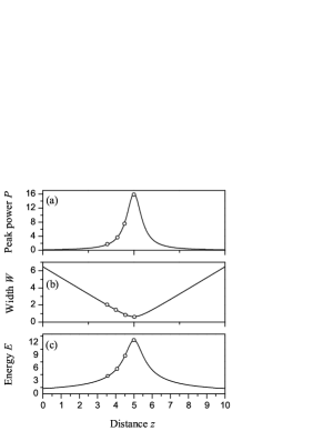
Figure 2: (Color online) The evolution of (a) the peak power, (b) FWHM, and (c) energy of the rogue wave with zero background. The parameters are the same as in Fig. 1.

Next, we aim to find out whether the fraction pulse can generate a soliton in the optical fiber Mahnke . For this purpose, we consider the dimensionless soliton number

$$N=\frac{W\sqrt{P}}{2\ln(1+\sqrt{2})},$$ (6)

where $P$ and $W$ are the initial peak power and FWHM for a sech-type pulse Agrawal . According to the standard soliton theory, any input pulse tends to eventually transform into a fundamental soliton if the soliton number falls into the interval of $0.5<N<1.5$. The breather wave form appears at $N\neq 1$. For the fraction pulse given by Eq. (4), it follows from expression (5) that its energy is $E\left(Z\right)=[\pi/(4\sqrt{\sqrt{2}-1})]P(Z)W(Z)$. It differs from energy $PW/\ln(1+\sqrt{2})$ of the sech-type pulse by factor $\pi\left(4\sqrt{\sqrt{2}-1}\right)^{-1}\ln\left(1+\sqrt{2}\right)\approx 1.076$. As this factor is close to $1$, the soliton number for this pulse can be approximately identified according to Eq. (6), which yields

$$N=\frac{W(Z)\sqrt{P(Z)}}{2\ln\left(1+\sqrt{2}\right)}=\frac{\sqrt{4(\sqrt{2}-1)}}{\ln\left(1+\sqrt{2}\right)}\approx 1.4604,$$ (7)

where $P(Z)$ and $W(Z)$ are given by Eq. (5). Thus, the emergence of a breather oscillating around a fundamental soliton is expected.

We take the fraction pulse at different positions $z\equiv z_{0}$ as the initial configuration, and simulate its subsequent evolution by numerically solving Eq. (1). The results are summarized in Fig. 3, which displays the subsequent evolution of the fraction pulse, initiated by its configurations which are taken, as said here, at different positions corresponding to $z_{0}=3.5$, $4$, $4.5$, and $5$. In Figs. 3(a) through 3(d), the pulses exhibit a typical oscillatory behavior of breathing solitons. With the increase of value $z_{0}$, at which the input is extracted from the fraction pulse (4), the oscillation period and width of the generated breather become smaller, while its power increases, as seen in Figs. 3(e) to 3(h). Thus, it is possible to create high-power pulses with different widths and peak powers by choosing appropriate input forms of the fraction pulse.

Figure 3: (Color online) The evolution of the rational fraction pulses, initiated by the configurations extracted from Eq. (4) at the corresponding positions: (a) $z_{0}=3.5$; (b) $z_{0}=4$; (c) $z_{0}=4.5$; (d) $z_{0}=5$ (see further details in the text). (e-h) The evolution of the corresponding pulse intensity and FWHM. The parameters are the same as in Fig. 1.

III Breather-like soliton generated by the spectral filtering

The above results, obtained for the completely integrable NLS equation, are relevant for picosecond pulses. In the femtosecond regime, higher-order effects, such as the third-order dispersion, self-steepening, self-frequency shift, and others, should be added to the model, transforming it into the higher-order NLS equation Kodama ; Agrawal :

$$\frac{\partial A}{\partial\xi}+i\frac{\beta_{2}}{2}\frac{\partial^{2}A}{\partial\tau^{2}}-\frac{\beta_{3}}{6}\frac{\partial^{3}A}{\partial\tau^{3}}$$

$$=i\gamma\left(|A|^{2}A+\frac{i}{\omega_{0}}\frac{\partial(|A|^{2}A)}{\partial\tau}-T_{R}A\frac{\partial|A|^{2}}{\partial\tau}\right),$$ (8)

where $A(\xi,\tau)$ is the slowly varying envelope of the electric field, $\tau$ and $\xi$ are the temporal coordinate and propagation distance, $\beta_{2}$ is the group-velocity dispersion, $\beta_{3}$ is the third-order dispersion, $\gamma$ is the Kerr nonlinearity coefficient of the fiber, $\omega_{0}$ is the central carrier frequency of the optical field, and $T_{R}$ is the Raman time constant. Here, we take realistic parameters for carrier wavelength $\lambda=1550$ nm, $\beta_{2}=-8.85\times 10^{-1}$ ps²/km, $\beta_{3}=1.331\times 10^{-2}$ ps³/km, $\gamma=10$ W${}^{-1}\cdot~{}$km^-1 Kibler , and $T_{R}=3$ fs, if the self-frequency shift is also considered.

By means of normalizations $A(\xi,\tau)=\sqrt{P_{0}}q(z,t)$, $t=\tau/T_{0}$, and $z=\xi/L_{D}$, with temporal scale $T_{0}=[\left|\beta_{2}\right|/(\gamma P_{0})]^{1/2}$ and dispersion length $L_{D}=(\gamma P_{0})^{-1}$, where $P_{0}$ is the initial power, Eq. (8) can be rewritten in the form

$$i\frac{\partial q}{\partial z}+\frac{1}{2}\frac{\partial^{2}q}{\partial t^{2}}+|q|^{2}q=i\alpha_{3}\frac{\partial^{3}q}{\partial t^{3}}+i\alpha_{4}\frac{\partial(|q|^{2}q)}{\partial t}+\alpha_{5}q\frac{\partial|q|^{2}}{\partial t},$$ (9)

where $\alpha_{3}=\beta_{3}/(6\left|\beta_{2}\right|T_{0})$, $\alpha_{4}=-(\omega_{0}T_{0})^{-1}$ and $\alpha_{5}=T_{R}/T_{0}$. When the higher-order terms in the right-hand side of Eq. (9) are absent, Eq. (9) reduces to Eq. (1). Here we take a typical value of the initial power, $P_{0}=0.3$ W, hence the other parameters are $T_{0}=0.543\,14$ ps, $L_{D}=1/3$ km, $\alpha_{3}=0.004\allowbreak 615$, $\alpha_{4}=-0.001\allowbreak 514$, and $\alpha_{5}=0.005523\allowbreak 4$.

As discussed in Ref. Ygy , the PS can be excited by a small localized (single-peak) perturbation pulse placed on top of a CW background. Here, as a typical example, we take the initial condition as a Gaussian-shaped perturbation pulse on the CW background

$$A(0,\tau)=\sqrt{P_{0}}[1+\epsilon\exp(-\tau^{2}/2T_{1}^{2})],$$ (10)

with amplitude $\epsilon$ and width $T_{1}$.

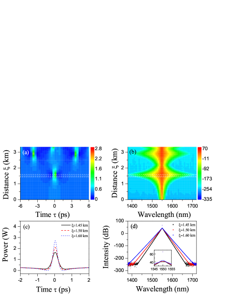
Figure 4: (Color online) The evolution of (a) the Peregrine rogue wave excited by initial condition (10), and (b) the corresponding evolution of its spectral intensity. (c) The growing temporal-domain pulse shapes and (d) the corresponding spectral shapes at $\xi=1.45$ km, $1.50$ km, and $1.60$ km, respectively. The parameters are $P_{0}=0.3$ W, $\epsilon=0.0765$, and $T_{1}=3.7722$ ps.

In the absence of the Raman effect, the evolution of the initial configuration (10) is presented in Fig. 4. The results show that the Gaussian perturbation on top of the CW background can excite a non-ideal Peregrine rogue wave, eventually evolving into the pulse-splitting regime due to the modulational instability of the CW background, as shown in Fig. 4(a). Figure 4(b) shows the corresponding evolution of the spectrum, which starts with narrow spectral components and then spreads into a triangular-type shape, similar to the so-called supercontinuum super . Then, the spectrum shrinks and spreads in the course of the propagation, but it does not recover the initial shape, due to the occurrence of the pulse splitting. This means that the Peregrine rogue wave cannot travel directly with a preserved shape, hence so it cannot be used for the design of a robust transmission scheme in optical fibers. For our choice of the parameters (which, as said above, are realistic for the applications), the largest compression of the pulse is attained at $\xi=1.60$ km, as shown in Fig. 4(c). The pulse’s intensity distributions at $\xi=1.45$ km, $1.50$ km, and $1.60$ km are presented in Fig. 4(c), and the corresponding spectral intensities are shown in Fig. 4(d), which shows that the spectrum of the background is mainly concentrated at $\lambda=1550$ nm.

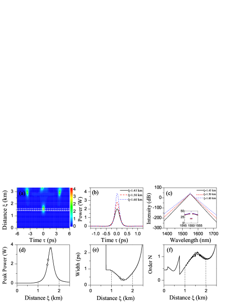
Figure 5: (Color online) (a) The evolution of the fraction pulse in the case when the background was removed from the Peregrine rogue wave. (b) and (c) The corresponding temporal and spectral shapes of the pulse at $\xi=1.45$ km, $1.50$ km, and $1.60$ km, respectively. (d), (e), and (f) The evolution of the peak power, FWHM, and soliton number $N$, respectively. The parameters are the same as in Fig. 4.

Figure 6: (Color online) (a), (c), and (e) The evolution of the initial state (10), corresponding to the fraction pulse, with the background extracted from the PS at (a) $\xi=1.45$ km, (c) $\xi=1.50$ km, and (e) $\xi=1.60$ km, respectively. (b), (d), and (f) The corresponding evolution of the peak power. Parameters of initial condition (10) are the same as in Fig. 4.

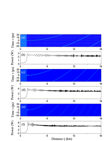
Figure 7: (Color online) The same as in Fig. 6, but with the Raman effect, with $T_{R}=3$ fs, taken into regard. The other parameters are the same as in Fig. 4.

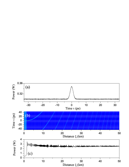
Figure 8: (Color online) The evolution of the breathing soliton extracted from the PS at $\xi=1.45$ km, under the the action of small perturbations added to initial condition (10). (a) The initial profile (10), perturbed by $0.1\%$ random noise. (b) The long-distance evolution of the pulse. (c) The corresponding evolution of the peak power. The parameters are the same as in Fig. 4.

Thus, to use the PS for the generation of high-power pulses with well-defined shapes, one needs to eliminate the background. Several ways for this, such as the use of the polarization technique, Raman effect, and interferometry, were previously proposed Stolen ; Mamyshev ; Fatome ; Mahnke . Here, we employ the spectral-filtering method to remove the background, as discussed in Ref. Ygy1 , in which the spectrum around $\lambda=1550$ nm was filtered out by attenuating its spectral intensity by $10\%$. Figure 5(a) displays the evolution of the fraction pulse, in which the background is filtered out in the range of $1$ nm around $1550$ nm. Such pulses are indeed surrounded by zero background, as seen in Fig. 5(b). The corresponding temporal and spectral intensity shapes at $\xi=1.45$ km, $1.50$ km, and $1.60$ km, are displayed in Figs. 5(b) and 5(c), respectively. Comparing with Figs. 4(c) and 4(d), we conclude that the temporal intensities of the fraction pulse are larger than those of the PS corresponding to the same propagation distances, $\xi=1.45$ km, $1.50$ km, and $1.60$ km, and the pulse’s spectrum is attenuated around $1550$ nm. The peak power and FWHM of such pulses are shown in Figs. 5(d) and 5(e). The respective soliton number $N$, given by formula (7), is plotted in Fig. 5(f). Open circles in panels 5(d-f) correspond to the sequence of growing pulses shown in Fig. 5(c). Note that the numerical results are valid only in the interval of $1<\xi<2$, because the filtered pulse does not exhibit a localized profile when the peak power is too small. In Fig. 5(f) one can see that the corresponding soliton numbers are all close to $N=1$ [see open circles in Fig. 5(f)], being obviously smaller than the numbers for the picosecond pulse, as the width of the pulses is smaller in the femtosecond regime.

Further, we have performed numerical simulations of the pulse evolution when the background was filtered out from the PS at propagation distances $\xi=1.45$ km, $\xi=1.50$ km, and $\xi=1.60$ km, respectively. The results are summarized in Fig. 6, which demonstrates that the pulses propagate stably over long propagation distances and exhibit the characteristic behavior of the breathing soliton. In particular, typical oscillatory evolution of the peak powers is shown in Figs. 6(b), 6(d), and 6(f).

Next, we consider the influence of the self-frequency-shift effect on the evolution of such pulses. The corresponding numerical results are displayed in Fig. 7, which shows the typical evolution of the pulses in the temporal domain, under the action of the Raman effect. Depending on the input, the evolving breathing solitons become narrower, whereas the peak powers increase accordingly, see Figs. 7(b), 7(d), and 7(f), respectively.

Finally, we consider the stability of the pulse against small random perturbations added to the initial background. In the numerical simulations, white-noise at the amplitude level of $0.1\%$ was added, as shown in Fig. 8(a). As a typical example, the evolution of the pulse which was extracted from the PS at $\xi=1.45$ km is shown in Figs. 8(b) and 8(c). Although the background around the breather was effectively removed at this point, the initial perturbations had a chance to contaminate the main fraction pulse. The results reveal that the initial random perturbations do not destabilize the generation and long-distance propagation of the breathing soliton.

IV Conclusions

Based on the analytic solution of the nonlinear Schrödinger equation in the form of the PS (Peregrine soliton, alias the Peregrine rogue wave), the evolution of a rational fraction pulse, extracted from that exact solution, has been analyzed in detail. The extensive numerical results have shown that the fraction pulse exhibits robust oscillatory (breather-like) propagation in the realistic model of nonlinear dispersive optical fibers. We have also investigated the generation and propagation of such breathing solitons extracted from the PS with the Raman self-frequency shift also taken into account. The numerical results clearly show that such solitons stably propagate in the optical fibers, being stable against random perturbations. The settings analyzed in this work can be experimentally implemented in the nonlinear fibers.

V Acknowledgement

This research is supported by the National Natural Science Foundation of China grant 61078079 and 61475198, the Shanxi Scholarship Council of China grant 2011-010 and the 331 Foundation of Basic Medical College of Shanxi Medical University. Qin is sponsored by Shanghai Pujiang Program (No. 14PJD007) and the Natural Science Foundation of Shanghai (No. 14ZR1403500).

References

- (1) D. H. Peregrine, J. Austral. Math. Soc. Ser. B 25, 16 (1983).
- (2) V. E. Zakharov, A. I. Dyachenko, and A. O. Prokofiev, Eur. J. Mech. B/Fluids 5, 677 (2006).
- (3) V. I. Shrira and Y. V. Geogjaev, J. Eng. Math. 67, 11 (2010).
- (4) U. Al Khawaja, H. Bahlouli, M. Asad-uz-zaman, and S. M. Al-Marzoug, Commun. Nonlinear Sci. Numer. Simulat. 19, 2706 (2014).
- (5) S. Chen and L.-Y. Song, Phys. Lett. A 378, 1228 (2014).
- (6) E. A. Kuznetsov, Sov. Phys. Dokl. 22, 507 (1977).
- (7) Ya. C. Ma, Stud. Appl. Math. 60, 43 (1979).
- (8) N. Akhmediev and V. I. Korneev, Theor. Math. Phys. 69, 1089 (1986).
- (9) C. Kharif and E. Pelinovsky, Eur. J. Mech. B/Fluids 22, 603 (2003).
- (10) A. Slunyaev, Eur. J. Mech. B/Fluids 25, 621 (2006).
- (11) V. P. Ruban, Phys. Rev. Lett. 99, 044502 (2007).
- (12) Andonowati, N. Karjanto, and E. van Groesen, App. Math. Mod. 31, 1425 (2007).
- (13) B. Kibler, J. Fatome, C. Finot, G. Millot, F. Dias, G. Genty, N. Akhmediev, and J. M. Dudley, Nature Physics 6, 790 (2010).
- (14) A. Chabchoub, N. P. Hoffmann, and N. Akhmediev, Phys. Rev. Lett. 106, 204502 (2011).
- (15) H. Bailung, S. K. Sharma, Y. Nakamura, Phys. Rev. Lett. 107, 255005 (2011).
- (16) K. Hammani, B. Kibler, C. Finot, Ph. Morin, J. Fatome, J. M. Dudley, and G. Millot, Opt. Lett. 36, 112 (2011).
- (17) N. J. Smith, F. M. Knox, N. J. Doran, K. J. Blow, and I. Bennion, Electron. Lett. 32, 54 (1996).
- (18) M. Nakazawa, H. Kubota, and K. Tamura, IEEE Photon. Technol. Lett. 8, 452 (1996).
- (19) T. Yu, E. A. Golovchenko, A. N. Pilipetskii, and C. R. Menyuk, Opt. Lett. 22, 793 (1997).
- (20) E. G. Shapiro and S. K. Turitsyn, Phys. Rev. E56, R4951 (1997).
- (21) S. K. Turitsyn, B. G. Bale, and M. P. Fedoruk, Phys. Rep. 521, 135 (2012).
- (22) B. A. Malomed, Soliton Management in Periodic Systems (Springer: New York, 2006).
- (23) V. N. Serkin and T. L. Belyaeva, JETP Lett. 74, 573 (2001).
- (24) V. N. Serkin and T. L. Belyaeva, Quantum Electron. 31 1007 (2001).
- (25) R. Hao, Lu Li, Z. Li, W. Xue, and G. Zhou, Opt. Commun. 236, 79 (2004).
- (26) V. I. Petviashvili and A. M. Sergeev, Dokl. AN SSSR 276, 1380 (1984) [Sov. Phys. Doklady 29, 493 (1984)].
- (27) B. A. Malomed, Physica D 29, 155 (1987).
- (28) R. J. Deissler and H. R. Brand, Phys. Rev. Lett. 72, 478 (1994).
- (29) S. Barland, J. R. Tredicce, M. Brambilla, L. A. Lugiato, S. Balle, M. Giudici, T. Maggipinto, L. Spinelli, G. Tissoni, T. Knödl, M. Miller, and R. Jäger, Nature (London) 419, 699 (2002); Z. Bakonyi, D. Michaelis, U. Peschel, G. Onishchukov, and F. Lederer, J. Opt. Soc. Am. B 19, 487 (2002); N. N. Rosanov, S. V. Fedorov, and A. N. Shatsev, Appl. Phys. B 81, 937 (2005); W. H. Renninger, A. Chong, and F. W. Wise, Phys. Rev. A 77, 023814 (2008); N. Veretenov and M. Tlidi, Phys. Rev. A 80, 023822 (2009); M. Tlidi, A. G. Vladimirov, D. Pieroux, and D. Turaev, Phys. Rev. Lett. 103, 103904 (2009); P. Genevet, S. Barland, M. Giudici, and J. R. Tredicce, Phys. Rev. Lett. 104, 223902 (2010); P. Grelu and N. Akhmediev, Nature Photonics, 6, 84 (2012); J. Jiménez, Y. Noblet, P. V. Paulau, D. Gomila, and T. Ackemann, J. Opt. 15, 044011 (2013); C. Fernandez-Oto, M. G. Clerc, D. Escaff, and M. Tlidi, Phys. Rev. Lett. 110, 174101 (2013).
- (30) M. Tlidi, M. Haelterman, and P. Mandel, Europhys. Lett. 42, 505 (1998); M. Tlidi and P. Mandel, Phys. Rev. Lett. 83, 4995 (1999); P. Mandel and M. Tlidi, J. Opt. B: Quantum Semiclass. Opt. 6, R60 (2004).
- (31) N. Akhmediev, J. M. Soto-Crespo, and G. Town, Phys. Rev. E63, 056602 (2001).
- (32) I. S. Aranson and L. Kramer, Rev. Mod. Phys. 74, 99 (2002); B. A. Malomed, in Encyclopedia of Nonlinear Science, p. 157. A. Scott (Ed.), Routledge, New York, 2005.
- (33) N. N. Rosanov, Spatial Hysteresis and Optical Patterns (Springer, Berlin, 2002).
- (34) V. Skarka and N. B. Aleksić, Phys. Rev. Lett. 96, 013903 (2006); N. B. Aleksić, V. Skarka, D. V. Timotijević, and D. Gauthier, Phys. Rev. A 75, 061802 (2007); D. Mihalache, D. Mazilu, F. Lederer, H. Leblond, and B. A. Malomed, Phys. Rev. A 77, 033817 (2008); V. Skarka, N. B. Aleksić, H. Leblond, B. A. Malomed, and D. Mihalache, Phys. Rev. Lett. 105, 213901 (2010); D. Mihalache, Proc. Rom. Acad. Ser. A 11, 142 (2010); Y. J. He and D. Mihalache, J. Opt. Soc. Am. B 29, 2554 (2012); D. Mihalache, Rom. J. Phys. 57, 352 (2012); V. Skarka, N. B. Aleksić, M. Lekić, B. N. Aleksić, B. A. Malomed, D. Mihalache, and H. Leblond, Phys. Rev. A 90, 023845 (2014); V. Besse, H. Leblond, D. Mihalache, and B. A. Malomed, Opt. Commun. 332, 279 (2014); Y. J. He, B. A. Malomed, and D. Mihalache, Phil. Trans. R. Soc. A 372, 20140017 (2014).
- (35) L. Song, H. Wang, L. Wu, and Lu Li, J. Opt. Soc. Am. B28, 86 (2011).
- (36) K. S. Bezuhanov, A. A. Dreischuh, and W. Królikowski, Phys. Rev. A77, 033825 (2006).
- (37) H. Zhang, Lu Li, and S. Jia, Phys. Rev. A76, 043833 (2007).
- (38) A. I. Strinić, M. S. Petrović, D. V. Timotijević, N. B. Aleksić, and M. R. Belić, Opt. Exp. 17, 11698 (2009).
- (39) N. B. Aleksić, M. S. Petrović, A. I. Strinić and M. R. Belić, Phys. Rev. A85, 033826 (2012).
- (40) M. S. Petrović, N. B. Aleksić, A. I. Strinić and M. R. Belić, Phys. Rev. A87, 043825 (2013).
- (41) A. Trombettoni and A. Smerzi, Phys. Rev. Lett. 86, 2353 (2001).
- (42) M. Matuszewski, E. Infeld, B. A. Malomed, and M. Trippenbach, Phys. Rev. Lett. 95, 050403 (2005).
- (43) M. Trippenbach, M. Matuszewski, E. Infeld, C. L. Van, R. S. Tasgal, Y. B. Band, Opt. Commun. 229, 391 (2004).
- (44) S. V. Gurevich, Sh. Amiranashvili, and H.-G. Purwins, Phys. Rev. E 74, 066201 (2006).
- (45) T. Bui Dinh, V. Cao Long, K. Dinh Xuan, and K. W. Wojciechowski, Phys. Stat. Sol. B 249, 1386 (2012).
- (46) N. Voglis, Mon. Not. R. Astron. Soc. 344, 575 (2003).
- (47) R. Driben, B. A. Malomed, A. V. Yulin, and D. V. Skryabin, Phys. Rev. A 87, 063808 (2013).
- (48) P. Li, L. Li, and B. A. Malomed, Phys. Rev. E 89, 062926 (2014).
- (49) Y. Fattal, A. Rudnick, and D. M. Marom, Opt. Express 19, 17298 (2011).
- (50) Y. Kodama and A. Hasegawa, IEEE J. Quantum Electron. 23, 510 (1987).
- (51) G. P. Agrawal, Nonlinear Fiber Optics. 4th edn. (Academic Press, 2007).
- (52) G. Y. Yang, L. Li, S. T. Jia, and D. Mihalache, Rom. Rep. Phys. 65, 902 (2013).
- (53) G. Y. Yang, L. Li, S. T. Jia, and D. Mihalache, Rom. Rep. Phys. 65, 391 (2013).
- (54) C. Mahnke and F. Mitschke, Appl. Phys. B 116, 15 (2014).
- (55) G. Y. Yang, L. Li, and S. T. Jia, Phys. Rev. E85, 046608 (2012).
- (56) D. V. Skryabin and A. V. Gorbach, Rev. Mod. Phys. 82, 1287 (2010).
- (57) R. H. Stolen, J. Botineau, and A. Ashkin, Opt. Lett. 7, 512 (1982).
- (58) P. V. Mamyshev, S. V. Chernikov, E. M. Dianov, and A. M. Prokhorov, Opt. Lett. 15, 1365 (1990).
- (59) J. Fatome, B. Kibler, and C. Finot, Opt. Lett. 38, 1663 (2013).