High-Activity Expansion for the Columnar Phase of the Hard Rectangle Gas

Abstract

We study a system of monodispersed hard rectangles of size $m\times d$, where $d\geq m$ on a two dimensional square lattice. For large enough aspect ratio, the system is known to undergo three entropy driven phase transitions with increasing activity $z$: first from disordered to nematic, second from nematic to columnar and third from columnar to sublattice phases. We study the nematic-columnar transition by developing a high-activity expansion in integer powers of $z^{-1/d}$ for the columnar phase in a model where the rectangles are allowed to orient only in one direction. By deriving the exact expression for the first $d+2$ terms in the expansion, we obtain lower bounds for the critical density and activity. For $m$, $k\gg 1$, these bounds decrease with increasing $k$ and decreasing $m$.

1 Introduction

A system of long rods in three dimensions with only excluded volume interactions is known to exhibit a density-driven phase transition from a disordered isotropic phase to an orientationally ordered nematic phase onsager ; flory ; z63 ; degennes ; vroege . Further increase in density may result in a smectic phase with orientational order and partial translational order, and a solid phase frenkel ; bolhuis . In two dimensional continuum space, the system undergoes a Berezinskii-Kosterlitz-Thouless transition b71 ; b72 ; kt73 from a low-density phase with exponential decay of correlations to a high-density phase where the correlations decay as a power law straley1971 ; frenkel1985 ; khandkar2005 ; vink2009 .

The corresponding problem has also been studied on lattices where the rods orient only along the lattice directions, and thus the number of allowed orientations is finite. In this case, it may be heuristically argued that the fully packed phase has no orientational order degennes ; deepak , making it uncertain whether a pure lattice model may ever exhibit a nematic phase degennes . There has been a renewed interest in this problem after it was convincingly demonstrated numerically that a system of hard rods on a square lattice exhibits a nematic phase for large enough aspect ratio deepak . Below, we summarize the known results for lattice models of hard rods and rectangles.

Consider a mono-dispersed system of hard rectangles of size $m\times d$ on a square lattice, where $k=d/m$ is the aspect ratio, and each rectangle may orient along one of two directions – horizontal or vertical. No two rectangles may overlap (see Sec. 2 for a more precise definition). When $m=1$ (hard rods), the system has been shown to undergo two density-driven transitions: a low-density isotropic–nematic transition shown numerically for $k\geq 7$ deepak and rigorously for $k\gg 1$ dg13 , and a second high-density nematic–disordered transition that has been shown numerically krds12 ; kundu2 . While the first transition is in the Ising universality class flr08 ; flr08a ; fernandez2008c ; linares2008 ; fischer2009 , there is no clear-cut evidence for the second transition belonging to any known universality class kundu2 . The $m=1$ model may be solved exactly on a tree-like lattice where the system undergoes an isotropic–nematic transition for $k\geq 4$, but the second transition is absent drs11 , though an exact solution for rods with soft repulsive interactions on the same lattice shows two transitions kr13 . The only other exact result is for $m=1$ and $k=2$ (dimers), where the absence of a transition for any density may be proved Heilmann1970 ; Kunz1970 ; Gruber1971 ; lieb1972 . The system with $m>1$ has also been studied. When $k=1$, and $m\geq 2$, the model reduces to the well-studied hard square model bellemans_nigam1nn ; bellemans_nigam3nn ; ree ; landau ; nisbet1 ; lafuente2003phase ; ramola ; schmidt ; slotte ; kinzel ; amar which undergoes a density-driven transition from a disordered to a columnar phase. The transition is continuous for $m=2$  fernandes2007 ; feng ; zhi2 and first order for $m=3$ fernandes2007 . The columnar phase breaks translational symmetry only in one lattice direction. When $m\geq 2$ and $k\geq 7$, the system undergoes three density-driven transitions: first an isotropic-nematic transition, second a nematic-columnar transition, and third a columnar-sublattice transition kundu3 ; kr14b . Here, the columnar phase breaks translational symmetry in the direction perpendicular to the nematic orientation. For $2\leq k<7$, and $m\geq 3$, the system undergoes isotropic-columnar and columnar-sublattice transitions with increasing density. When $m=2$, the system undergoes a direct isotropic-sublattice transition for $k=2,3$ kundu3 .

In this paper, we focus on the nematic-columnar transition. When $m=2$, the critical density $\rho_{c}$ (the fraction of occupied lattice sites) for this transition was numerically determined for $d$ up to $48$. By extrapolating to $d\to\infty$, it was shown that $\rho_{c}\approx 0.727+0.226k^{-1}+O(k^{-2})$ kr14b , implying the existence of the columnar phase for infinitely long rectangles. It is difficult to study systems with larger $m$ using Monte Carlo simulations as it becomes difficult to equilibrate the systems at large densities, restricting the numerical study of large $k$ to $m=2$. The nematic-columnar transition has also been studied analytically within a Bethe approximation kundu3 . While this calculation qualitatively reproduces the above numerical result, the approximations involved are ad-hoc with no clear systematic procedure of improving the results. In addition, the limit $m\to\infty$ keeping $k=d/m$ fixed, corresponding to a system of oriented rectangles in the continuum, is unattainable. As of now, unlike the nematic phase, there exists no rigorous proof for the existence of the columnar phase.

High-activity expansions are a systematic and more rigorous way of studying the effect of fluctuations in the ordered state. In the standard Mayer expansion, the high-activity expansion is in integer powers of $z^{-1}$, where $z$ is the activity or fugacity gaunt_fisher . However, columnar phases possess a sliding instability resulting in the expansion being in fractional powers of $z^{-1}$ bellemans_nigam1nn . The expansion was carried out to $O(z^{-3/2})$ for the hard square gas ($m=2$, $d=2$) recently ramola , and the formalism was applied to hard core lattice gas models with first four next nearest neighbor exclusion, where the high-density phase is columnar trisha .

In this paper, we generalize the calculations of the hard square gas in Ref. ramola to derive the high-activity expansion for the columnar phase of the hard rectangle gas. To do so, we study a simpler model where rectangles may orient only in the horizontal direction. We justify this simplification by arguing that near the nematic-columnar transition, there are only a few rectangles with orientation perpendicular to the nematic orientation. In addition, we also show that the nematic-columnar transition densities are the same for large $k$ (within numerical error), whether both orientations or only one orientation is allowed. We show that the high-activity expansion is in powers of $z^{-1/d}$, where $z$ is the activity or fugacity. The exact expressions for the first $d+2$ terms in the expansion of free energy and densities are derived. Truncating the expansions for the densities at this order, we obtain estimates (lower bounds) for the critical densities for the nematic-columnar transition. For large $m$ and $k$, these estimates are shown to decrease with increasing $k$ and decreasing $m$.

The rest of the paper is organized as follows. Section 2 contains a definition of the model and the justification for studying a model of hard rectangles with only horizontal orientation. The high-activity expansion for the free energy of $m\times d$ rectangles is derived in Sec. 3. In Sec. 4, we derive the high-activity expansion for the occupation densities of the different rows. The critical densities, and activities are estimated from these expansions. Section 5 contains a discussion of the results and some possible extensions of the problem.

2 Model and Preliminaries

Consider a square lattice of size $L\times L$ with periodic boundary conditions. We consider a system of monodispersed hard rectangles of size $m\times d$, where $k=d/m$ is the aspect ratio, and $d\geq m$. A horizontal (vertical) rectangle occupies $d$ ($m$) consecutive lattice sites along the $x$-direction and $m$ ($d$) consecutive lattice sites along the $y$-direction. No lattice site may be occupied by more than one rectangle. The grand canonical partition function for the system is

$$\overline{\mathcal{L}}(z_{h},z_{v})=\sum\limits_{n_{h},n_{v}}\overline{C}(n_{h},n_{v})z_{h}^{n_{h}}z_{v}^{n_{v}},$$ (1)

where $\overline{C}(n_{v},n_{h})$ is the number of valid configurations with $n_{h}$ horizontal rectangles and $n_{v}$ vertical rectangles, and $z_{h}$ and $z_{v}$ are the corresponding activities.

In the nematic and columnar phases, the orientational symmetry is broken, and thus the majority of rectangles are either horizontal or vertical. Typical snapshots of the system ($m=2$, $d=18$) at equilibrium near the nematic-columnar transition are shown in Fig. 1. The system has nearly complete orientational order, and one may ignore the effects of the rectangles with perpendicular orientation. To study the nematic–columnar phase transition, it is thus more convenient to study a system in which all rectangles are horizontal. Thus, we set $z_{v}=0$ in (1), disallowing vertical rectangles.

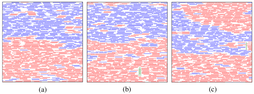
Figure 1: Snapshots of a system of rectangles of size $2\times 18(k=9)$ at Monte Carlo time steps (a) $7\times 10^{7}$, (b) $8\times 10^{7}$, and (c) $9\times 10^{7}$. Red and blue- are horizontal rectangles with heads at the even and odd rows respectively and green are vertical rectangles.

Further justification of this simplification may be obtained by comparing the critical density $\rho_{c}$ for the nematic-columnar transition for the model of rectangles with both orientations and the model of rectangles with only horizontal orientation. $\rho_{c}$ for the model with both orientations allowed was numerically obtained for $m=2$ as $\rho_{c}\approx 0.727+0.226k^{-1}$ for $k\gg 1$ kr14b . Here, we obtain $\rho_{c}$ for the model restricted to horizontal rectangles from Monte Carlo simulations. The details of the algorithm and parameters are as in Refs. kundu3 ; kr14b . $\rho_{c}$ is obtained for $m=2$ by the intersection point of the Binder cumulant for three different lattice sizes, and is shown in Fig 2. We obtain $\rho_{c}\approx 0.727+0.226k^{-1}$ for $k\gg 1$, numerically indistinguishable from that for the model with both horizontal and vertical rectangles. We thus conclude that the simplified model is well-suited for studying the nematic-columnar transition. However, it is possible that the two models have qualitatively different phenomenology for small $k$ when the nematic phase is absent for the model with both orientations allowed (also see Sec. 5 for more discussion of this point).

Figure 2: The critical density $\rho_{c}$ for the nematic-columnar transition for the model with only horizontal rectangles (circles) and the model with both horizontal and vertical rectangles (squares) from Monte Carlo simulation. The data for the latter is from Ref. kr14b . The straight line is $0.727+0.226k^{-1}$. Inset: The corresponding critical activity $z_{c}$ from Monte Carlo simulation. The straight line is $35.5k^{-1}$.

Let the bottom left corner of a rectangle be called its head. In the nematic phase, each row on an average contains equal number of heads of rectangles. In the columnar phase, this symmetry is broken. An example illustrating the two phases for $2\times 6$ rectangles is shown in Fig. 3. To quantify the nematic–columnar transition, we assign to the $i^{th}$ row a label $(i\mod m)+1$, such that the labels are $1,\ldots,m$. In the columnar phase, majority of the rectangles have their heads on one of the $m$ types of rows. The grand canonical partition function for the model with only horizontal rectangles is then

$$\mathcal{L}(\{z_{i}\})=\sum_{n_{1},\ldots,n_{m}}C(n_{1},\ldots,n_{m})\prod_{i=1}^{m}z_{i}^{n_{i}},$$ (2)

where $C(n_{1},\ldots,n_{m})$ is the number of configurations with $n_{i}$ rectangles whose heads are on rows with label $i$, and $z_{i}$’s are the corresponding activities. For large activities, the system will be in the columnar phase, and undergoes a transition to the nematic phase as the activities are decreased.

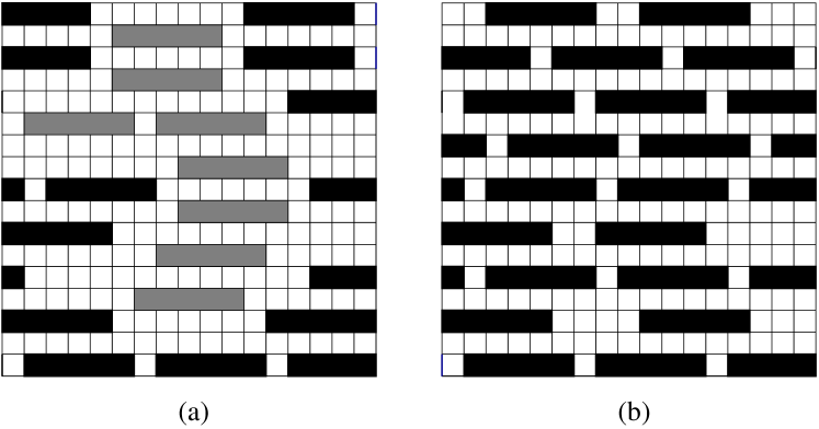
Figure 3: A schematic diagram illustrating the two phases for $2\times 6$ rectangles. (a) The low activity nematic phase where some of the heads (bottom left corner) of the rectangles are on odd rows (black) and some of the heads are on even rows (grey). (b) The high activity columnar phase where most of the heads of rectangles are either on even or odd rows (odd in the example shown).

The free energy of the system in the thermodynamic limit is

$$f(z_{1},\ldots,z_{m})=\lim_{N\to\infty}-\frac{1}{N}\ln\mathcal{L}(z_{1},\ldots,z_{m}),$$ (3)

where $N=L^{2}$ is the total number of lattice sites. The density of occupied sites $\rho$ is then given by

$$\rho(z)=-mdz\frac{d}{dz}f(z,\ldots,z).$$ (4)

The aim of the paper is to determine the free energy $f$ and density $\rho$ as a perturbation series in inverse powers of the activity.

3 High activity expansion for the free energy

The perturbation series for the free energy will be in powers of $z^{-1/d}$ [see Sec. 3.1 and (19)] rather than the usual Mayer expansion in integer powers of $z^{-1}$ because of the ordered columnar phase having a sliding instability bellemans_nigam1nn ; ramola . Suppose a vacancy is created in a fully ordered columnar phase at full packing by removing a rectangle. The $d$ consecutive empty sites that are created may now be broken into $d$ fractional vacancies without any loss of entropy by sliding sets of rectangles in the horizontal direction. This breaking up of vacancies into fractional vacancies leads to fractional powers of $z^{-1}$ appearing in the perturbation expansion.

To set up a perturbation expansion about the ordered columnar state, it is convenient to choose one of the activities to be large and treat the other activities as small parameters:

$$z_{1}=z_{o},$$ (5)

$$z_{2}=\ldots=z_{m}=z_{e},$$ (6)

where $z_{e}\ll z_{o}$. The notation is such that when $m=2$, $o$ indicates odd rows and $e$ indicates even rows. Once the perturbation expansion is obtained, $z_{o}$ and $z_{e}$ are equated to $z$ to obtain the high-activity expansion.

In the completely ordered state, heads of all the rectangles are in rows with label $1$ [see Fig. 3(b)]. In the perturbation expansion, we refer to rectangles whose heads are in rows with a label different from $1$ as defects. For systems with sliding instability, the perturbation expansion is not in terms of number of defects, but rather in terms of clusters of defects bellemans_nigam1nn ; ramola . We illustrate this for the case $m=2$. Consider a single defect on a row with label $2$ [see Fig. 4(a)]. This defect results in one or more rectangles removed from each of the two rows denoted by $\ast$ in Fig. 4(a), both with label $1$, and therefore has leading weight $z^{-1}$. Now consider two defects both on rows with label $2$ but one directly above the other [see Fig. 4(b)]. This cluster of defects results in one or more rectangles removed from each of the three rows denoted by $\ast$ in Fig. 4(b), all three with label $1$, and therefore still has leading weight $z^{-1}$. It is easy to see that a similar defect cluster of arbitrary size will have leading weight $z^{-1}$. When $m>2$, defect-clusters may have defects with different labels (as defined below). For such clusters, it is again possible that defect-clusters of different sizes also have leading weight $z^{-1}$.

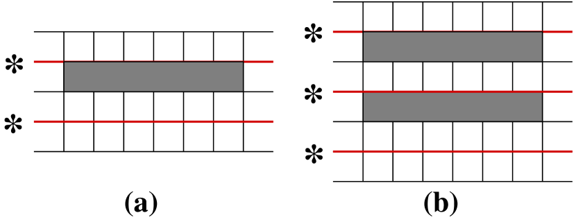
Figure 4: A schematic diagram illustrating clusters. (a) One rectangle on an even row results in reducing the maximal occupancy of two odd rows (red lines labeled *) by one. (b) Two rectangles on even rows one directly above the other results in reducing the maximal occupancy of three odd rows (red lines labeled *) by one.

We define a single cluster of defects more precisely. Let a sub-cluster of size $n$ and label $j$ denote a set of $n$ rectangles of label $j$, directly on top of each other such that the long sides are parallel and the short sides are aligned. A single cluster of defects is made up of sub-clusters of label $2,3,\ldots m$, such that the labels are in ascending order and the gap between two sub-clusters is the minimum possible. Examples of single clusters of size $4$ for $3\times 6$ rectangles are shown in Fig. 5. In Fig. 5(a), the cluster is made up of a single sub-cluster of label $2$ while in Fig. 5(b), the cluster is made up of one sub-cluster of size 2 of label $2$ and one sub-cluster of size $2$ of label $3$. It is straightforward to check that all such single cluster of defects will have leading weight $z^{-1}$.

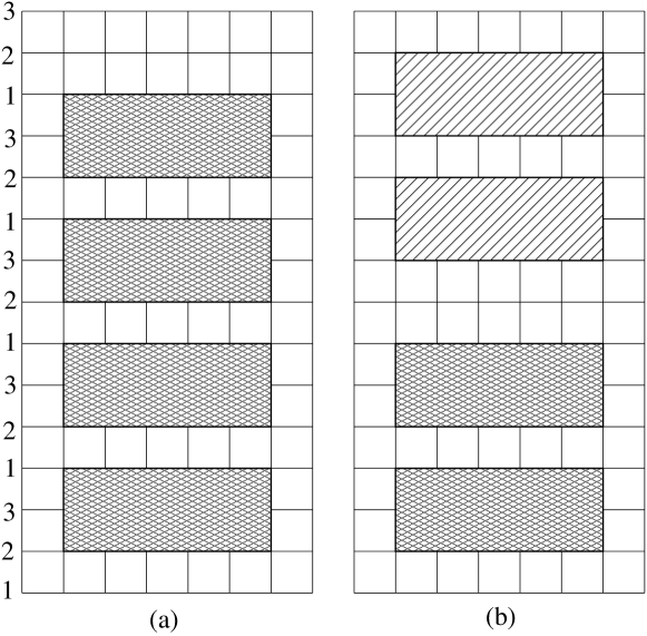
Figure 5: An example of a single cluster of size $4$ made up of (a) 4 defects of label 2 and (b) 2 defects of label 2 and 2 defects of label 3. The example is for rectangles of size $3\times 6$.

The perturbation expansion is well-defined in terms of number of clusters bellemans_nigam1nn ; ramola . Thus, we write

$$\frac{\mathcal{L}(z_{o},z_{e})}{\mathcal{L}(z_{o},0)}=1+W_{1}(z_{o},z_{e})+W_{2}(z_{o},z_{e})+\ldots,$$ (7)

where $W_{n}$ represents the contribution from $n$ clusters. The free energy may then written as a series:

$$f(z_{o},z_{e})=f_{0}(z_{o})+f_{1}(z_{o},z_{e})+f_{2}(z_{o},z_{e})+\ldots,$$ (8)

where $f_{i}$ corresponds to the contribution from $i$ clusters. From (3), we immediately obtain

$$f_{0}(z_{o}) =\frac{-1}{N}\ln\mathcal{L}(z_{o},0),$$ (9)

$$f_{1}(z_{o},z_{e}) =\frac{-1}{N}W_{1}(z_{o},z_{e}),$$ (10)

$$f_{2}(z_{o},z_{e}) =\frac{-1}{N}\left[W_{2}(z_{o},z_{e})-\frac{W_{1}(z_{o},z_{e})^{2}}{2}\right].$$ (11)

The free energies $f_{0}$, $f_{1}$ and $f_{2}$ are calculated in the following subsections.

3.1 Calculation of $f_{0}$

$f_{0}$ is the contribution to the free energy from configurations that do not have defects. Then the heads of all the rectangles are in rows with label $1$ and the configuration in a particular row is independent of the configurations in other rows, Hence, we can write

$$\mathcal{L}(z_{o},0)=\left[\Omega_{p}(z_{o},L)\right]^{L/m},$$ (12)

where $\Omega_{p}(z_{o},L)$ is the grand canonical partition function of a system of hard rods of length $d$ on a one dimensional lattice of $L$ sites with periodic boundary condition. The one dimensional partition function obeys simple recursion relations. $\Omega_{p}(z_{o},L)$ is related to $\Omega_{o}(z_{o},L)$, the corresponding grand canonical partition function on a one dimensional lattice of $L$ sites with open boundary conditions, as

$$\Omega_{p}(z,L)=dz\Omega_{o}(z,L-d)+\Omega_{o}(z,L-1),~{}L\geq d.$$ (13)

$\Omega_{o}(z,\ell)$ obeys the following recursion relation:

$$\Omega_{o}(z,\ell) =z\Omega_{o}(z,\ell-d)+\Omega_{o}(z,\ell-1),~{}\ell\geq d,$$ (14)

$$\Omega_{o}(z,\ell) =1,~{}0\leq\ell<d.$$ (15)

Equation (14) is solved by the ansatz $\Omega_{o}(z,\ell)=A\lambda^{\ell}$, where $A$ is a constant. Substituting into (14), we obtain

$$\lambda^{d}-\lambda^{d-1}-z=0.$$ (16)

Let $\lambda_{1}$ denote the largest root of (16). For arbitrary $d$, $\lambda_{1}$ may be solved as a perturbation series in inverse powers of $z^{-1}$. By examining a few terms in the expansion, we find that the series solution of $\lambda_{1}$ has the following form:

$$\lambda_{1}(z)=z^{1/d}+\frac{1}{d}+\sum_{n=1}^{\infty}\frac{z^{-n/d}}{d^{n+1}(n+1)!}\prod_{j=1}^{n}(jd-n).$$ (17)

The free energy $f_{0}$ is related to the $\lambda_{1}$ as

$$f_{0}=-\frac{1}{m}\ln\lambda_{1}(z_{0}).$$ (18)

Thus,

$$f_{0}=-\frac{\ln z_{o}}{dm}-\frac{z_{o}^{-1/d}}{dm}-\sum_{n=2}^{\infty}\frac{z_{o}^{-n/d}}{n!d^{n}m}\prod_{j=1}^{n-1}(jd-n).$$ (19)

Note that $f_{0}$ is a series in integer powers of $z_{o}^{-1/d}$ rather than the usual Mayer expansion that is in integer powers of $z_{o}^{-1}$.

It will turn out later that, to calculate the contribution from configurations with two defect-clusters, we will need knowledge of the partition function $\Omega_{o}(z,\ell)$ for all $\ell$ and not just for large $\ell$ when only the largest root $\lambda_{1}$ of (16) contributes. $\Omega_{o}(z,\ell)$ is a linear combination of the $d$ roots of (16). Denoting the roots by $\lambda_{n}$,

$$\Omega_{o}(z,\ell)=\sum\limits_{n=1}^{d}c_{n}\lambda_{n}^{\ell},$$ (20)

where $c_{n}$ are constants to be determined from (15). Substituting (20) in (15) we obtain

$$\begin{pmatrix}1&1&1&\ldots&1\\ \lambda_{1}&\lambda_{2}&\lambda_{3}&\ldots&\lambda_{d}\\ \lambda_{1}^{2}&\lambda_{2}^{2}&\lambda_{3}^{2}&\ldots&\lambda_{d}^{2}\\ \ldots&\ldots&\ldots&\ldots&\ldots\\ \ldots&\ldots&\ldots&\ldots&\ldots\\ \lambda_{1}^{d-1}&\lambda_{2}^{d-1}&\lambda_{3}^{d-1}&\ldots&\lambda_{d}^{d-1}\end{pmatrix}\begin{pmatrix}c_{1}\\ c_{2}\\ \cdot\\ \cdot\\ \cdot\\ c_{d}\end{pmatrix}=\begin{pmatrix}1\\ 1\\ \cdot\\ \cdot\\ \cdot\\ 1\end{pmatrix}.$$ (21)

By inverting the Vandermonde matrix in (21), we obtain

$$c_{n}=(-1)^{d-1}\frac{\prod\limits_{\begin{subarray}{c}j=1\\ j\neq n\end{subarray}}^{d}(\lambda_{j}-1)}{\prod\limits_{\begin{subarray}{c}j=1\\ j\neq n\end{subarray}}^{d}(\lambda_{n}-\lambda_{j})},$$ (22)

To obtain $c_{n}$’s as a series in $z_{o}^{-1/d}$, we need to first obtain all $\lambda_{n}$’s as a series in $z_{o}^{-1/d}$. From (16), we immediately notice that $|\lambda_{n}|=z^{1/d}$, $z\to\infty$. Let

$$\lambda_{n}=z^{1/d}e^{i\theta_{n}}.$$ (23)

Substituting into (16), we obtain

$$e^{i\theta_{n}d}=1+z^{-1/d}e^{i\theta_{n}(d-1)}.$$ (24)

The perturbative solution to (24) is straightforward to obtain:

$$\lambda_{n}=z^{1/d}e^{i\theta_{n}}+\frac{1}{d}+\frac{(d-1)e^{-i\theta_{n}}}{2d^{2}}z^{-1/d}+O(z^{-2/d}),$$ (25)

where

$$\theta_{n}=\frac{2(n-1)\pi}{d},\quad n=1,2,\ldots,d.$$ (26)

Using the expression for $c_{n}$’s in (22), we obtain

$$c_{n}=\frac{1}{d}+\frac{(d-1)e^{-i2\pi(n-1)/d}}{d^{2}}z^{-1/d}+\ldots,~{}n=1,\ldots,d.$$ (27)

3.2 Calculation of $f_{1}$

A single cluster of defects of size $n$ consists of $n$ rectangles placed one directly above the other, keeping the long sides parallel, with the heads being in rows with labels $2,\ldots,m$ (see text before (7) for a more precise definition). Given a defect-cluster of size $n$, the occupation of exactly $n+1$ rows with label $1$ are affected. The contribution to $W_{1}$ from a single defect cluster of size $n$ is then $\left[\frac{\Omega_{o}(z_{o},L-d)}{\Omega_{p}(z_{o},L)}\right]^{n+1}z_{e}^{n}$. The bottom left corner of the cluster has to be on a row with label $2$, and there are $N/m$ ways of choosing this lattice site. In addition, we need to account for the number of ways $H(n)$ that a cluster of size $n$ may be split into sub-clusters with different labels. The number of ways of distributing $n$ rectangles into $m-1$ sub-clusters, where the sub-clusters are arranged in ascending order of labels, is

$$H(n)={n+m-2\choose m-2}.$$ (28)

Thus, the contribution to $W_{1}$ from configurations with a single cluster of defects is

$$W_{1}(z_{o},z_{e}) =\frac{N}{m}\sum\limits_{n=1}^{\infty}H(n)\left[\frac{\Omega_{o}(z_{o},L-d)}{\Omega_{p}(z_{o},L)}\right]^{n+1}z_{e}^{n},$$ (29)

$$=\frac{N}{m}\frac{\Omega_{o}(z_{o},L-d)}{\Omega_{p}(z_{o},L)}\left[\frac{1}{\left[1-\frac{z_{e}\Omega_{o}(z_{o},L-d)}{\Omega_{p}(z_{o},L)}\right]^{m-1}}-1\right].$$ (30)

$\Omega_{p}(z_{o},L)$ may be expressed in terms of $\Omega_{o}(z_{o},L)$ using (13):

$$\Omega_{p}(z_{o},L)\> =\>\Omega_{o}(z_{o},L-d)\left[dz_{o}+\frac{\Omega_{o}(z_{o},L-1)}{\Omega_{o}(z_{o},L-d)}\right],$$ (31)

$$\underset{L\to\infty}{=}\Omega_{o}(z_{o},L-d)\left[dz_{o}+\lambda_{1}^{d-1}\right].\$$ (32)

where in the limit $L\to\infty$, we used $\Omega_{o}(z_{o},\ell)\sim\lambda_{1}^{\ell}$. Substituting into (30), using (10), setting $z_{e}=z_{o}=z$, and expanding for large $z$, we obtain,

$$f_{1}(z,z) = \frac{-1}{mdz}\left[\frac{d^{m-1}}{(d-1)^{m-1}}-1\right]+\frac{1}{md^{2}z^{1+1/d}}\left[\frac{d^{m-1}(d+m-2)}{(d-1)^{m}}-1\right]$$ (33)

$$+O\left(\frac{1}{z^{1+2/d}}\right).$$

Thus single clusters of defects contribute at $O(z^{-1})$.

3.3 Calculation of $f_{2}$

$f_{2}$ is the contribution to the free energy from two defect-clusters. There are four types of possible configurations:

1. Clusters that are separated by at least one row of label $1$ that may be occupied with rectangles independent of other rows.

2. Clusters that intersect.

3. Clusters that do not have any overlap in the $y$-direction, and are not of type (a) or (b).

4. Clusters that have some overlap in the $y$-direction, and are not of type (b).

We calculate the contribution from each of these types in the following subsections.

3.3.1 Type (a): Clusters that are separated from each other

The contribution of clusters of type (a) to the free energy is exactly cancelled by the contribution from the product of two single clusters $W_{1}^{2}$ [which is $O(z^{-2})$]. Thus, there is no contribution to the free energy.

3.3.2 Type (b): Clusters that intersect

When two clusters intersect, $W_{2}$ is exactly zero since such configurations are forbidden. However, there is a contribution to $f_{2}$ from such configurations through the terms $W_{1}^{2}$. Since $W_{1}$ is $O(z^{-1})$, the contribution to $f_{2}$ is $O(z^{-2})$. Later, we will not be keeping terms of $O(z^{-2})$, and we therefore neglect the contribution to $f_{2}$ from such configurations.

3.3.3 Type (c): Clusters that do not overlap in the $y$-direction

Let $W_{2}^{x}(z_{o},z_{e})$ denote the contribution to $W_{2}(z_{o},z_{e})$ from configurations of clusters that have no overlap in the $y$-direction, but may overlap in the $x$-direction. Examples of such configurations are shown in Fig. 6. Let the number of defects in the clusters be denoted by $n_{a}$ and $n_{b}$, and let $\Delta$ denote the distance in the $x$ direction between the centers of the two clusters, where $\Delta\geq 1$. When $\Delta<d$, the two clusters have some overlap in the $x$-direction [see Fig. 6(a)], otherwise not [see Fig. 6(b)].

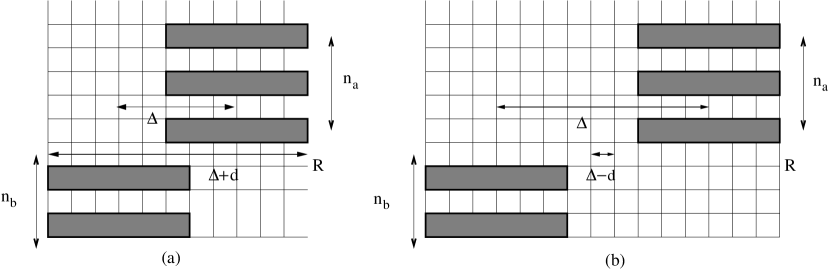
Figure 6: Examples of configurations of two clusters with no overlap in the $y$-direction. $\Delta$ is the distance between the centers of the two clusters in the $x$-direction. Clusters could overlap in the $x$-direction as in (a) $1\leq\Delta<d$, or have no overlap in the $x$-direction as in (b) $\Delta\geq d$.

Let $t_{1}$ ($t_{2}$) denote the contribution to $W_{2}^{x}$ from pairs with $\Delta<d$ ($\Delta\geq d$). We calculate $t_{1}$ and $t_{2}$ separately. For $t_{1}$, not all pairs of clusters with the same $\Delta$ contribute at the same order in $z$. The lowest order contribution appears from pair of clusters where the smallest label of the defects in the upper cluster is larger than or equal to largest label of the defects in the lower cluster. Other pairs of clusters contribute at $O(z^{-2})$. This may be easily seen in the example shown in Fig 7, where two cluster configurations are shown for the case $m=3$. In Fig 7(a), the largest label of lower cluster is $3$ and the smallest label of the upper cluster is also $3$. Such a configuration of four defects affects five rows of label $1$ (denoted by bold lines) and contributes at $O(z^{-1})$. In Fig 7(b), the largest label of lower cluster is $3$ but the smallest label of the upper cluster is now $2$. Such a configuration of four defects affects six rows of label $1$ (denoted by bold lines), contributing at $O(z^{-2})$.

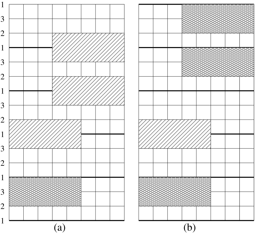
Figure 7: Examples of configurations with two defect-clusters when $m=3$. (a) The lower cluster has two defects of labels $2$ and $3$ while the upper cluster has two defects of label $3$. Such a configuration affects the occupation of five rows of label $1$ (shown by bold lines). (b) The upper clusters has two defects of label $2$. Such a configuration affects the occupation of $6$ rows of label $1$ (shown by bold lines).

For the calculation of $t_{1}$, we will, therefore, restrict ourselves to cluster configurations where the smallest label of the defects in the upper cluster is larger than or equal to largest label of the defects in the lower cluster. In this case, the upper cluster may be slid to the left by $\Delta$ till the two clusters merge to form a single cluster. Thus, the combinatorial factor associated with dividing the two clusters into sub-clusters of different labels is, as in the case of single clusters [see Sec. 3.2 and (28)], $H(n_{a}+n_{b})$, where $n_{a}$ and $n_{b}$ are the number of defects in the top and bottom clusters respectively. For $t_{2}$ ($\Delta\geq d$), the labels in each cluster are independent of each other, and the combinatorial factor is therefore equal to $H(n_{a})H(n_{b})$. In addition, for both $t_{1}$ and $t_{2}$, since we restrict $\Delta\geq 1$, a symmetry factor $2$ is associated with each configuration.

We now calculate the contribution to $t_{1}$ and $t_{2}$ from the occupation of rows of label $1$ with rectangles. The occupation of $n_{a}+n_{b}+1$ rows of label 1 with rectangles are affected by the presence of the defects. The remaining rows of label $1$ may be filled independently of each other. Among the $n_{a}+n_{b}+1$ rows, other than the row marked by $R$ in Fig. 6(a) and (b), $n_{a}+n_{b}$ rows may be thought of as open chains of length $L-d$. When $\Delta<d$ [see Fig. 6(a)], the row R is equivalent of an open chain of length $L-d-\Delta$. When $\Delta\geq d$ [see Fig. 6(b)], the row R is equivalent of two open chains of lengths $\Delta-d$ and $L-2d-(\Delta-d)$. Thus, we obtain

$$t_{1}=\frac{2N}{m}\sum\limits_{n_{a},n_{b}=1}^{\infty}\!\!H(n_{a}+n_{b})\left[\frac{\Omega_{o}(z_{o},L-d)z_{e}}{\Omega_{p}(z_{o},L)}\right]^{n_{a}+n_{b}}\sum\limits_{\Delta=1}^{d-1}\frac{\varOmega_{o}(z_{o},L-d-\Delta)}{\varOmega_{p}(z_{o},L)},$$ (34)

and

$$t_{2} =\frac{2N}{m}\sum\limits_{n_{a},n_{b}=1}^{\infty}H(n_{a})H(n_{b})\left[\frac{\Omega_{o}(z_{o},L-d)z_{e}}{\Omega_{p}(z_{o},L)}\right]^{n_{a}+n_{b}}$$

$$\times\sum\limits_{\Delta=d}^{\infty}\frac{\Omega_{o}(z_{o},L-d-\Delta)\Omega_{o}(z_{o},\Delta-d)}{\Omega_{p}(z_{o},L)},$$ (35)

where the factor $N/m$ accounts for the number of ways of placing the lower cluster on sublattice $2$.

In the limit $L\to\infty$, $\Omega_{p}(z_{o},L)$ may be expressed in terms of $\Omega_{o}(z_{o},L)$ using (32). The limit of large $L$ does not apply to the term $\Omega_{o}(z_{o},\Delta-d)$, as $\Delta-d$ may be as small as zero. Hence, we use (20) for the one dimensional partition function for any length. We, then, obtain

$$t_{1}=\frac{2N}{m}\sum\limits_{n_{a},n_{b}=1}^{\infty}H(n_{a}+n_{b})\left[\frac{z_{e}}{dz_{o}+\lambda_{1}^{d-1}}\right]^{n_{a}+n_{b}}\sum\limits_{\Delta=1}^{d-1}\frac{\lambda_{1}^{-\Delta}}{dz_{o}+\lambda_{1}^{d-1}},$$ (36)

and

$$t_{2}=\frac{2N}{m}\sum\limits_{n_{a},n_{b}=1}^{\infty}H(n_{a})H(n_{b})\left[\frac{z_{e}}{dz_{o}+\lambda_{1}^{d-1}}\right]^{n_{a}+n_{b}}\sum\limits_{\Delta=d}^{\infty}\sum\limits_{j=1}^{d}\frac{c_{1}\beta_{j}\alpha_{j}^{\Delta-d}}{\lambda_{1}^{d}(dz_{o}+\lambda_{1}^{d-1})},$$ (37)

where

$$\beta_{j} =\frac{c_{j}}{c_{1}},$$ (38)

$$\alpha_{j} =\frac{\lambda_{j}}{\lambda_{1}},$$ (39)

with $c_{j}$ and $\lambda_{j}$ as defined in (20). Knowing the perturbation expansion for $c_{j}$ [see (27)] and $\lambda_{j}$ [see (17) and (25)], the perturbation expansion for $\beta_{j}$ and $\alpha_{j}$ may be derived to be

$$\beta_{j} =1+\frac{d-1}{dz_{o}^{1/d}}\left[e^{-i2\pi(j-1)/d}-1\right]+O(z_{o}^{-2/d}),~{}j=2,\ldots,d,$$ (40)

$$\alpha_{j} =e^{i\theta_{j}}+\frac{1}{dz_{o}^{1/d}}(1-e^{i\theta_{j}})+O(z_{o}^{-2/d}),~{}j=2,\ldots,d,$$ (41)

$$\frac{1}{1-\alpha_{j}} =\frac{1}{1-e^{i\theta_{j}}}\left(1+\frac{1}{dz_{o}^{1/d}}\right)+O(z_{o}^{-2/d}),~{}j=2,\ldots,d,$$ (42)

where $\theta_{j}$ is as defined in (26).

We now focus on $t_{2}$ [see (37)]. Since $|\alpha_{j}|<1$ for $j>1$, the sum over $\Delta$ reduces to a convergent geometric series for $j>1$. Summing over $\Delta$, we obtain

$$t_{2} =\frac{2N}{m}\sum\limits_{n_{a},n_{b}=1}^{\infty}H(n_{a})H(n_{b})\left(\frac{z_{e}}{dz_{o}+\lambda_{1}^{d-1}}\right)^{n_{a}+n_{b}}$$

$$\times\left[\sum\limits_{\Delta=d}^{\infty}\frac{c_{1}}{\lambda_{1}^{d}(dz_{o}+\lambda_{1}^{d-1})}+\sum\limits_{j=2}^{d}\frac{c_{1}\beta_{j}}{\lambda_{1}^{d}(dz_{o}+\lambda_{1}^{d-1})(1-\alpha_{j})}\right]$$ (43)

Though the first term in (3.3.3) is divergent, in the calculation for $f_{2}$, it may be checked that this term is cancelled by the term $-W_{1}^{2}/2$. From (27) $c_{1}\sim d^{-1}$, and (40) $\beta_{j}\sim O(1)$. Similarly $|\alpha_{j}|\sim 1$, though $\alpha_{j}\neq 1$ for $j>1$ [see (41)]. Also $\lambda_{1}\sim z^{1/d}$ [see (17)]. Therefore, we obtain that the second term in (3.3.3) is $O(z_{o}^{-2})$. Therefore, we conclude that $t_{2}\sim O(z^{-2})$.

In the expression for $t_{1}$ [see (36)], the leading order of the term for a fixed $\Delta$ is $z^{1+\Delta}$. Keeping only the $\Delta=1$ term, we obtain

$$W_{2}^{x}=\frac{2N}{m}\sum\limits_{n_{a},n_{b}=1}^{\infty}\frac{H(n_{a}+n_{b})}{dz_{o}^{1+1/d}}\left(\frac{z_{e}}{dz_{o}}\right)^{n_{a}+n_{b}}+O(z^{-1-2/d}).$$ (44)

Doing the summation and setting $z_{e}=z_{o}=z$, we obtain

$$W_{2}^{x}=\frac{2N}{mdz^{1+1/d}}\left[1-\frac{d^{m-1}(d-m)}{(d-1)^{m}}\right]+O(z^{-1-2/d}).$$ (45)

3.3.4 Type (d): Clusters that overlap in the $y$-direction

Two non-intersecting rectangles of different labels are said to overlap in the $y$-direction if the $y$-coordinate of the head of the rectangle with larger label lies within the $y$-range of the rectangle with smaller label. Two rectangles of same label are said to overlap in the $y$-direction if their heads are on the same row. Two defect-clusters are said to overlap in the $y$-direction if they contain at least one pair of overlapping rectangles. Let $W_{2}^{y}$ denote the contribution from configurations with two defect-clusters that have some overlap in the $y$-direction. We divide such configurations into four types, as shown in Fig. 8, with their contributions to $W_{2}^{y}$ being denoted by $p_{1}$, $p_{2}$, $p_{3}$ and $p_{4}$. In $p_{1}$, neither of the clusters has any extension beyond the common section. In $p_{2}$, one of the clusters extends beyond the common section in one direction. In $p_{3}$, both clusters extend beyond the common section in mutually opposite directions, while in $p_{4}$, one cluster extends beyond the common section in both directions. Each of the two clusters are single clusters as defined in 3.2 (also see Fig. 4). The configurations of type $p_{2}$, $p_{3}$ and $p_{4}$ may occur in four, two and two ways respectively, depending on which of the clusters is extending beyond the common section and in which direction.

Figure 8: Four possible cases of two clusters with overlap along $y$. In $p_{1}$, both clusters do not extend beyond the common section. In $p_{2}$, one of the clusters extends beyond the common section in one direction. In $p_{3}$, both clusters extend beyond the common section. In $p_{4}$, one of the clusters extends beyond the common section in both directions. The numbers come from symmetry considerations and is straightforward to obtain.

For a pair of clusters, let $n_{0}$ denote the number of rectangles that overlap in the $y$-direction. Let the number of rectangles in the sections extending above and below the common section be denoted by $n_{a}$ and $n_{b}$ respectively. As in Sec. 3.3.3, let $\Delta$ be the horizontal distance between the centers of the two clusters. Clearly $\Delta\geq d$. These symbols are illustrated in an example in Fig. 9.

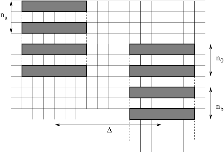
Figure 9: An example ($m=2$, $d=7$) illustrating the definition of $n_{0}$, $n_{a}$, $n_{b}$, and $\Delta$. $n_{0}$ is the number of rectangles in the common section ($2$ in example), $n_{a}$ and $n_{b}$ are the extensions above and below ($2$ each) and $\Delta$ is the horizontal distance between the centers of the two clusters ($10$ in example).

We now calculate $p_{1}$, $p_{2}$, $p_{3}$ and $p_{4}$. For $p_{1}$, the presence of the defect-clusters affects the occupation of exactly $(n_{0}+1)$ rows of label $1$. The occupation of each of these rows with rectangles is equivalent to occupying two open chains of length $\Delta-d$ and $L-d-\Delta$. Also, for each of the clusters, the number of ways of breaking it up into sub-clusters is $H(n_{0})$. Thus,

$$p_{1}=\frac{N}{m}\sum\limits_{n_{0}=1}^{\infty}\sum\limits_{\Delta=d}^{\infty}H(n_{0})^{2}\left[\frac{\varOmega_{o}(z_{o},L-d-\Delta)\varOmega_{o}(z_{o},\Delta\!-\!d)}{\varOmega_{p}(z_{o},L)}\right]^{n_{0}+1}\!\!\!z_{e}^{2n_{0}}.$$ (46)

Expressing $\Omega_{p}$ in terms of $\Omega_{o}$ using (32), and $\Omega_{o}(z_{o},\Delta-d)$ in terms of $\lambda_{j}$ using (20), we obtain

$$p_{1}=\frac{N}{m}\sum\limits_{n_{0}=1}^{\infty}\sum\limits_{\Delta=d}^{\infty}H(n_{0})^{2}\left[\frac{c_{1}\sum\limits_{\begin{subarray}{c}j=1\end{subarray}}^{d}\beta_{j}\alpha_{j}^{\Delta-d}}{\lambda_{1}^{d}(dz_{o}+\lambda_{1}^{d-1})}\right]^{n_{0}+1},$$ (47)

where $\beta_{j}$ and $\alpha_{j}$ are as defined in (40) and (41). Expanding the last term in (47) using multinomial expansion, we obtain

$$p_{1} =\frac{N}{m}\sum\limits_{n_{0}=1}^{\infty}H(n_{0})^{2}z_{e}^{2n_{0}}\left[\frac{c_{1}}{\lambda_{1}^{d}(dz_{o}+\lambda_{1}^{d-1})}\right]^{n_{0}+1}$$

$$\times\sideset{}{{}^{\prime}}{\sum}\limits_{\{n_{l}\}\geq 0}\frac{(n_{0}+1)!}{\prod\limits_{j=1}^{d}n_{j}!}\sum\limits_{\Delta=d}^{\infty}\prod\limits_{p=2}^{d}(\beta_{p}\alpha_{p}^{\Delta-d})^{n_{p}},$$ (48)

where the primed sum refers to the constraint

$$\sum\limits_{i=1}^{d}n_{i}=n_{0}+1.$$ (49)

Summing over $\Delta$, we obtain

$$p_{1}=\frac{N}{m}\sum\limits_{n_{0}=1}^{\infty}H(n_{0})^{2}z_{e}^{2n_{0}}\left[\frac{c_{1}\lambda_{1}^{-d}}{dz_{o}+\lambda_{1}^{d-1}}\right]^{n_{0}+1}\sideset{}{{}^{\prime}}{\sum}\limits_{\{n_{l}\}\geq 0}\frac{(n_{0}+1)!\prod\limits_{p=2}^{d}\beta_{p}^{n_{p}}}{\prod\limits_{s=1}^{d}n_{s}![1-\prod\limits_{j=2}^{d}\alpha_{j}^{n_{j}}]}.$$ (50)

We now estimate the order of the different terms in (50). From (27) $c_{1}\sim 1/d$ and from (25), $\lambda_{1}^{d}\sim z_{o}$. Hence

$$\frac{c_{1}\lambda_{1}^{-d}}{dz_{o}+\lambda_{1}^{d-1}}\sim\frac{1}{(dz_{o})^{2}}.$$ (51)

To leading order, $\beta_{i}=1$, for all $i$ [see (40)]. Hence, unless the term $1-\prod_{j=2}^{d}\alpha_{j}^{n_{j}}$ in (50), goes to zero as $z\to\infty$, the summand is $O(z^{-2})$. Since we are not interested in terms of $O(z^{-2})$, we focus only on those $\{n_{l}\}$ for which $\prod_{j=2}^{d}\alpha_{j}^{n_{j}}\approx 1$, when $z\to\infty$. We obtain from (41)

$$\prod\limits_{j=2}^{d}\alpha_{j}^{n_{j}}=e^{\sum\limits_{j=2}^{d}i\theta_{j}n_{j}}\left[1-\sum\limits_{j=2}^{d}\frac{(1-e^{-i\theta_{j}})n_{j}}{dz_{o}^{1/d}}\right]+O(z_{0}^{-2/d}).$$ (52)

We are interested in those $\{n_{l}\}$ for which the leading term of the product is $1$. This leads to the constraint

$$\sum\limits_{j=2}^{d}\theta_{j}n_{j}=2l\pi,\quad l\in\mathbb{Z},$$ (53)

such that,

$$1-\prod\limits_{j=2}^{d}\alpha_{j}^{n_{j}}=\sum\limits_{j=2}^{d}\frac{(1-e^{-i\theta_{j}})n_{j}}{dz_{o}^{1/d}}.$$ (54)

Let

$$I(n_{0})=\sideset{}{{}^{\prime\prime}}{\sum}\limits_{\{n_{l}\}\geq 0}\frac{1}{\prod\limits_{j=1}^{d}n_{j}!\sum\limits_{j=2}^{d}(1-e^{-i\theta_{j}})n_{j}},$$ (55)

where the double prime refers to the constraints (49) and (53). It is straightforward to see that $I(n_{0})$ is real. $\alpha_{j}$’s appear as complex conjugate pairs. For every $\{n_{l}\}$ satisfying the constraints, there is a $\{n^{\prime}_{l}\}$ obtained by interchanging the $n_{l}$’s of all complex conjugate pairs, the corresponding summand being the complex conjugate. Thus $I(n_{0})$ is real. Equation (50) then reduces to

$$p_{1}=\frac{N}{m}\sum\limits_{n_{0}=1}^{\infty}H(n_{0})^{2}\left(\frac{z_{e}}{dz_{o}}\right)^{2n_{0}}\frac{(n_{0}+1)!I(n_{0})}{dz_{o}^{2-1/d}}+O(z^{-2}).$$ (56)

Thus $p_{1}$ is of order $z^{2-1/d}$ and for $d>2$ does not contribute to order $z^{1+1/d}$.

For configurations of type $p_{2}$, one of the clusters extends beyond the other, the two clusters being of length $n_{o}$ and $n_{0}+n_{a}$, where the common section in the $y$-direction has $n_{o}$ rectangles. The presence of these defect-clusters affects the occupation of $(n_{o}+n_{a}+1)$ rows of label $1$. Out of these rows, $n_{o}+1$ of them are equivalent to open chains of length $\Delta-d$ and $L-d-\Delta$, and the remaining $n_{a}$ are equivalent to an open chain of length $L-d$. The number of ways of dividing the clusters into sub-clusters is $H(n_{0}+n_{a})H(n_{0})$. In addition, there is a factor of $4N/m$ from symmetry considerations. Thus,

$$p_{2} =\frac{4N}{m}\sum\limits_{n_{0},n_{a}=1}^{\infty}\sum\limits_{\Delta=d}^{\infty}H(n_{0})H(n_{0}+n_{a})z_{e}^{2n_{0}+n_{a}}$$

$$\times\left[\frac{\varOmega_{o}(z_{o},L-d)}{\varOmega_{p}(z_{o},L)}\right]^{n_{a}}\left[\frac{\varOmega_{o}(z_{o},L-d-\Delta)\varOmega_{o}(z_{o},\Delta-d)}{\varOmega_{p}(z_{o},L)}\right]^{n_{0}+1}.$$ (57)

For configurations of type $p_{3}$, both clusters extend beyond the common section in the $y$-direction, one cluster being of length $n_{0}+n_{a}$ and the other being of length $n_{0}+n_{b}$. The number of ways of dividing the clusters into sub-clusters is $H(n_{0}+n_{a})H(n_{0}+n_{b})$. For configurations of type $p_{4}$, one cluster extends beyond the common section in both directions, one cluster being of length $n_{0}+n_{a}+n_{b}$ and the other being of length $n_{0}$. The number of ways of dividing the clusters into sub-clusters is $H(n_{0}+n_{a}+n_{b})H(n_{0})$. For both $p_{3}$ and $p_{4}$ the presence of the defect-clusters affects the occupation of $(n_{o}+n_{a}+n_{b}+1)$ rows of label $1$. Out of these rows, $n_{o}+1$ of them are equivalent to open chains of length $\Delta-d$ and $L-d-\Delta$, and the remaining $n_{a}+n_{b}$ are equivalent to an open chain of length $L-d$. Each of these two types also has an additional factor of $2N/m$ due to symmetry considerations. Thus, we obtain

$$p_{3} =\frac{2N}{m}\sum\limits_{n_{a}=1}^{\infty}\sum\limits_{n_{b}=1}^{\infty}\sum\limits_{\Delta=d}^{\infty}\sum\limits_{n_{0}=1}^{\infty}H(n_{0}+n_{a})H(n_{0}+n_{b})z_{e}^{2n_{0}+n_{a}+n_{b}}$$

$$\times\left[\frac{\varOmega_{o}(z_{o},L-d)}{\varOmega_{p}(z_{o},L)}\right]^{n_{a}+n_{b}}\left[\frac{\varOmega_{o}(z_{o},L-d-\Delta)\varOmega_{o}(z_{o},\Delta-d)}{\varOmega_{p}(z_{o},L)}\right]^{n_{0}+1},$$ (58)

and

$$p_{4} =\frac{2N}{m}\sum\limits_{n_{a}=1}^{\infty}\sum\limits_{n_{b}=1}^{\infty}\sum\limits_{\Delta=d}^{\infty}\sum\limits_{n_{0}=1}^{\infty}H(n_{0}+n_{a}+n_{b})H(n_{0})z_{e}^{2n_{0}+n_{a}+n_{b}}$$

$$\times\left[\frac{\varOmega_{o}(z_{o},L-d)}{\varOmega_{p}(z_{o},L)}\right]^{n_{a}+n_{b}}\left[\frac{\varOmega_{o}(z_{o},L-d-\Delta)\varOmega_{o}(z_{o},\Delta-d)}{\varOmega_{p}(z_{o},L)}\right]^{n_{0}+1}.$$ (59)

The expressions for $p_{2}$ [see (3.3.4)], $p_{3}$ [see (58)] and $p_{4}$ [see (59)] are similar to that for $p_{1}$ [see (46)] except for the factor $z_{e}^{n_{a}+n_{b}}[\varOmega_{o}(z_{o},L-d)/\varOmega_{p}(z_{o},L)]^{n_{a}+n_{b}}$. However, this factor is $O(z^{0})$. Hence, $p_{2}$, $p_{3}$, and $p_{4}$ are also of $O(z^{-2+1/d})$. Combining the contributions from $p_{1}$, $p_{2}$, $p_{3}$ and $p_{4}$, we obtain

$$W_{2}^{y} =\frac{N}{m}\left[\sum\limits_{n_{0}=0}^{\infty}H(n_{0})^{2}+4\sum\limits_{n_{0}=0}^{\infty}\sum\limits_{n_{a}=1}^{\infty}H(n_{0})H(n_{0}+n_{a})\left(\frac{z_{e}}{dz_{o}}\right)^{n_{a}}\right.$$

$$+2\sum\limits_{n_{0}=0}^{\infty}\sum\limits_{n_{a}=1}^{\infty}\sum\limits_{n_{b}=1}^{\infty}\left[H(n_{0}+n_{a})H(n_{0}+n_{b})+H(n_{0}+n_{a}+n_{b})H(n_{0})\right]$$

$$\left.\left(\frac{z_{e}}{dz_{o}}\right)^{n_{a}+n_{b}}\right]\left(\frac{z_{e}}{dz_{o}}\right)^{2n_{0}}\frac{(n_{0}+1)!I(n_{0})}{dz_{o}^{2-1/d}}+O(z^{-2}).$$ (60)

3.3.5 Expression for $f_{2}$

The contribution to the free energy $f_{2}$ from clusters with two configurations may now be computed. $W_{2}^{x}$ [see (45)] contributes at order $z^{-1-1/d}$. It is straightforward to argue that configurations with three clusters will contribute at utmost order $z^{-1-2/d}$, hence we truncate $f_{2}$ at order $z^{-1-1/d}$. The leading term of $W_{2}^{y}$ is $O(z^{-2+1/d})$, which for $d>2$ is much smaller than $W_{2}^{x}$. Hence $W_{2}^{y}$ does not contribute to $f_{2}$ for $d>2$. When $m=2$ and $d=2$ we should include $O(z^{-2+1/d})$ term in $W_{2}^{y}$. This equals $3\ln(9/8)$, and coincides with the high-activity expansion for $2\times 2$ hard squares ramola . Substituting for $W_{2}^{x}$ from (45), we obtain

$$f_{2}=\frac{-2}{mdz^{1+1/d}}\left[1-\frac{d^{m-1}(d-m)}{(d-1)^{m}}+6\delta_{d,2}\ln\frac{9}{8}\right]+O(z^{-1-2/d}).$$ (61)

3.4 High activity expansion for the free energy

The free energy up to order $z^{-1-1/d}$ is obtained by summing $f_{0}$ [(19)], $f_{1}$ [(33)], and $f_{2}$ [(61)]:

$$-f(z,z) =\frac{\ln z}{dm}+\frac{z^{-1/d}}{dm}+\sum_{n=2}^{d+1}\frac{z^{-n/d}}{n!d^{n}m}\prod_{j=1}^{n-1}(jd-n)+\frac{z^{-1}}{md}\left(\kappa-1\right)$$

$$+\frac{z^{-1-1/d}}{md^{2}}\left[1+2d-\frac{\kappa\left(2d^{2}-2dm+d+m-2\right)}{d-1}+24\delta_{d,2}\ln\frac{9}{8}\right]$$

$$+O(z^{-1-2/d}).$$ (62)

where

$$\kappa=\left(\frac{d}{d-1}\right)^{m-1}.$$ (63)

4 Densities and transition points

In this section we derive the high-activity expansion for the occupation densities of different rows. We truncate these expressions at $O(z^{-1-1/d})$ and then estimate the critical densities and activities for the nematic-columnar transition, and obtain their dependence on $m$ and $k$.

Let $\rho_{o}$ ($\rho_{e}$) denote the number of lattice sites occupied by rectangles whose heads are in rows with label $1$ (label different from $1$). For rows with labels different from $1$, the occupation densities will be equal. Hence,

$$\rho_{o}=-mdz_{o}\frac{d}{dz_{o}}f(z_{o},z_{e}),$$ (64)

$$\rho_{e}=\frac{-mdz_{e}}{m-1}\frac{d}{dz_{e}}f(z_{o},z_{e}),$$ (65)

where the factor $md$ accounts for the volume of a rectangle, and the factor $m-1$ accounts for the $m-1$ labels that are different from $1$. We, thus, obtain (after setting $z_{o}=z_{e}=z$)

$$\rho_{o} =1-\frac{z^{-1/d}}{d}-\sum\limits_{n=2}^{d+1}\frac{z^{-n/d}}{d^{n}(n-1)!}\prod_{j=1}^{n-1}(jd-n)+\frac{1}{z}\left[1-\frac{\kappa(d+m-2)}{d-1}\right]$$

$$-\frac{(2d+1)(d+1)}{d^{2}z^{1+1/d}}-\frac{\kappa}{(d-1)^{2}z^{1+1/d}}\Big{[}\frac{m-2}{d^{2}}-\frac{m^{2}-m+1}{d}$$

$$+2m^{2}-5m+6+(2m-1)d-2d^{2}+(17\ln\frac{9}{8}+4)\delta_{d,2}\Big{]}+O(z^{-1-2/d}),$$ (66)

$$\rho_{e} =\kappa\left[\frac{1}{z(d-1)}+\frac{2md-2d-m+2+(16\ln\frac{9}{8}+8)\delta_{d,2}}{d(d-1)^{2}z^{1+1/d}}\right]+O(z^{-1-2/d}),$$ (67)

where $\kappa$ is as defined in (63).

In Fig. 10 we plot (66) and (67), truncated at $O(z^{-1-1/d})$ for $m=2$ and $d=22$. With increasing $z^{-1}$, $\rho_{o}$ decreases while $\rho_{e}$ increases. The intersection point of these two curves gives an estimate of the transition point. In the example shown in Fig. 10, the estimates for the critical parameters are $z_{c}\approx 0.267$ and $\rho_{c}\approx 0.411$, where $z_{c}$ and $\rho_{c}$ are the critical activity and critical density respectively.

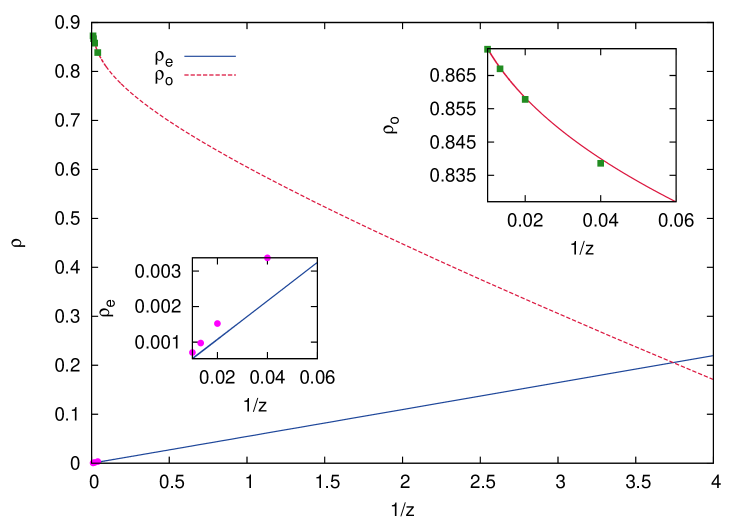
Figure 10: The high activity expansions (66) and (67) for $\rho_{o}$ and $\rho_{e}$ truncated at order $z^{-1-1/d}$ for $m=2$ and $d=22$. The data points are from Monte Carlo simulations. The two curves intersect at $z_{c}\approx 0.267$ and $\rho_{c}=\rho_{o}+\rho_{e}\approx 0.411$. Right inset: Blow up of the large $z$ region for $\rho_{o}$. Left inset: Blow up of the large $z$ region for $\rho_{e}$.

For large $z$, the expressions (66) and (67) are a good approximation to the actual densities and reproduce the Monte Carlo results quite accurately. The comparison with the Monte Carlo results is in shown in the insets of Fig. 10 for both $\rho_{o}$ and $\rho_{e}$, and in Table 1 for $\rho$. For $z\geq 25.0$, the expansion matches with the Monte Carlo results up to the third decimal place. This serves as an additional check for the correctness of the calculations.

Table 1: Comparison of the results for density $\rho$ from the high-activity expansion $\rho^{exp}$ [see (66) and (67)] with results from Monte Carlo simulations $\rho^{sim}$ for four different values of the activity $z$. The data are for a system of $2\times 22$ rectangles.

z	$\rho^{exp}$	$\rho^{sim}$
25.0	0.8422	0.8420
50.0	0.8594	0.8593
75.0	0.8680	0.8680
100.0	0.8736	0.8736

By truncating the high-activity expansion, $\rho_{o}$ is overestimated and $\rho_{e}$ is underestimated. In addition, for $m>3$, the nematic-columnar transition is first order in nature ($\rho$ has a discontinuity), and $z_{c}$ will be larger than the value of $z$ for which $\rho_{o}=\rho_{e}$. Hence, the estimate for $z_{c}$ that we obtain by setting $\rho_{o}=\rho_{e}$ in the truncated series is a lower bound to the actual $z_{c}$. For example, for $2\times 2$ rectangles, $z_{c}$ increases from $6.250$ when the series are truncated at $O(z^{-1})$ to $14.859$ when the series are truncated at $O(z^{-1-1/d})$ while the actual value is $97.5$ ramola , while for $2\times 22$ rectangles the corresponding values are $0.253$, $0.267$, and $2.11$ (see Fig. 2) respectively. We find that the increase in $z_{c}$, when terms of $O(z^{-1-1/d})$ are included, scales as $k^{-2}$, while the corresponding increase in $\rho_{c}$ scales as $k^{-1}$.

We now study the dependence of the estimated $z_{c}$ and $\rho_{c}$ on $m$ and $d$. Figure 11 shows the variation of $z_{c}$ with $k$ for different values of $m$. For large $k$, $z_{c}$ decreases with $k$ as a power law $ck^{-1}$, where $c\approx 2.78$ is independent of $m$. For small $k$, there is a crossover to a different behavior that depends weakly on $m$. We could not collapse the data for different $m$ onto a single curve by scaling $k$ with a power of $m$. Hence, most likely the crossover scale increases logarithmically with $m$. To summarize,

$$z_{c}\approx\frac{2.78}{k},\quad k\gg 1,\quad\forall m.$$ (68)

This behavior is in qualitative agreement with the result from Monte Carlo simulation where $z_{c}\approx 35.5k^{-1}$ (see Fig. 2).

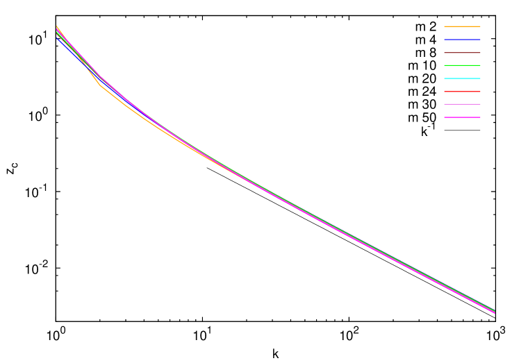
Figure 11: Variation of $z_{c}$ with $k$ for different $m$.

The variation of the corresponding critical density $\rho_{c}(m,k)$ with $k$ and $m$ is shown in Fig. 12. For large $k$, $\rho_{c}$ decreases linearly with $k^{-1}$ for all $m$. This dependence is brought out more clearly by $d\rho_{c}/dk=\rho_{c}(k+1)-\rho_{c}(k)$ (see left inset of Fig. 12), which is independent of $m$ and decreases as $k^{-2}$ for large $k$. We may thus write

$$\rho_{c}(m,k)=\rho_{c}(m,\infty)+\frac{b_{1}}{k},\quad k\gg 1,$$ (69)

where $\rho_{c}(m,\infty)$ is the $m$-dependent critical density for systems of rectangles of infinite aspect ratio, and $b_{1}\approx 0.367$ is independent of $m$. For the corresponding data from Monte Carlo simulation $b_{1}\approx 0.226$ (see Fig. 2). We determine $\rho_{c}(m,\infty)$ by fitting the data to (69), and its dependence on $m$ is shown in the right inset of Fig. 12. We find that the data is well-described by the form

$$\rho_{c}(m,\infty)\approx b_{2}-\frac{b_{3}}{\ln(m+b_{4})},~{}m\gg 1,$$ (70)

with $b_{2}\approx 0.464$, $b_{3}\approx 0.29$ and $b_{4}\approx 13.0$.

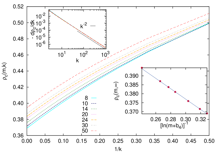
Figure 12: Variation of $\rho_{c}(m,k)$ with $k$ for different $m$. Right inset: $\rho_{c}(m,\infty)$, the critical density for rectangles with infinite aspect ratio, is well-described by (70) $b_{2}=0.464$, $b_{3}=0.29$, and $b_{4}=13.0$ (fit shown by solid line). Left inset: The data for $d\rho_{c}/dk$ for different $m$ collapse onto a single curve, independent of $m$.

Note that the $k$-dependence of $\rho_{c}(m,k)$ [see (69)] is in qualitative agreement with the results from Monte Carlo simulations for systems with $m=2$ (see Fig. 2 and kr14b ) and those from Bethe approximation for large $k$ kundu3 . Thus, though the estimates that we obtain are lower bounds for the actual transition, we expect that the truncated expansions give the correct qualitative trends for the critical parameters.

We now study the large $m$ behavior of the critical density and critical activity of system of hard squares of size $m\times m$, i.e., $k=1$. We find that $z_{c}$ increases up to $m=97$ and then decreases to a constant for large $m$, while $\rho_{c}(m,1)$ decreases up to $m=19$ and then increases to a constant for large $m$. The asymptotic critical values are approached logarithmically as the data are best described by (see Fig. 13)

$$z_{c}(m,1) =b_{5}+\frac{b_{6}}{\ln(m+b_{7})},$$ (71)

$$\rho_{c}(m,1) =b_{8}-\frac{b_{9}}{\ln(m+b_{10})},$$ (72)

with $b_{5}=12.085$, $b_{6}=9.54$, $b_{7}=228.56$, $b_{8}=0.669$, $b_{9}=0.44$, and $b_{10}=121.24$.

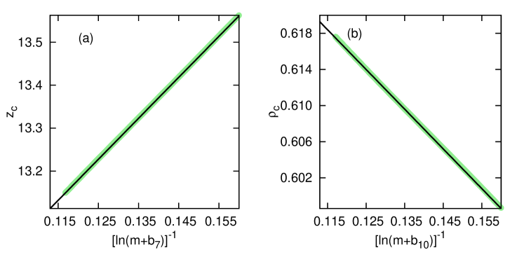
Figure 13: Critical (a) activity $z_{c}$, and (b) density $\rho_{c}$, for a system of $m\times m$ hard squares. The straight lines correspond to (a) (71) with $b_{5}=12.085$, $b_{6}=9.54$ and $b_{7}=228.56$, and (b) (72) with $b_{8}=0.669$, $b_{9}=0.44$ and $b_{10}=121.24$.

5 Conclusions and discussion

In this paper, we derived the high-activity expansion for the free energy and density of the columnar phase of $m\times d$ rectangles in a model where the rectangles were restricted to be horizontal. The expansion is in inverse powers of $z^{-1/d}$, where $z$ is the activity. We explicitly computed the first $d+2$ terms in this expansion. As in the case for hard squares ($m=2$, $d=2$) ramola , the expansion is not in terms of single defects, but in terms of clusters of defects.

From the high-activity expansions for the densities of rectangles with heads on rows of different labels, truncated at $O(z^{-1-1/d})$, we estimate the transition points $z_{c}$ and $\rho_{c}$. We show that $z_{c}\approx ck^{-1}$, $\rho_{c}(m,k)\approx\rho_{c}(m,\infty)+b_{1}k^{-1}$ for $k\gg 1$, where $c>0$, and $b_{1}>0$, are $m$-independent constants, and $\rho_{c}(m,\infty)$ increases logarithmically to a constant at large $m$. For hard squares with $d=m$, or equivalently $k=1$, we obtain that the critical density increases logarithmically to a constant when $m\gg 1$.

The high-density series being truncated at $O(z^{-1-1/d})$, the estimates for the critical parameters are lower bounds for the actual values. However, we note that the dependence of $\rho_{c}(m,k)$ and $z_{c}(m,k)$ on $k$ matches qualitatively with the results obtained from Monte Carlo simulations for $m=2$ (see Fig. 2 and kr14b ) and Bethe approximation kundu3 for large $k$. This leads us to conjecture that the trends for the critical parameters obtained from the truncated series expansion are qualitatively correct. If that is true, the limit $m\to\infty$ keeping the aspect ratio $k$ fixed, corresponding to the limit of oriented rectangles in the continuum may be studied. When $m\to\infty$, our results show that $z_{c}$ decreases to a finite constant for all $k$. If this feature carries over to the actual system, then, it would imply that $\rho_{c}$ for large $m$ is less than one, implying that the nematic-columnar transition should exist when $m\to\infty$. Likewise, there should be a isotropic-columnar transition for hard squares ($k=1$) in the continuum at a finite density. These conjectures should be verifiable using Monte Carlo for systems in the continuum.

The high density expansion derived in this paper was for a model where all the rectangles were horizontal. This is a special case ($z_{v}=0$) of the more general model where rectangles of horizontal and vertical orientations occur with activity $z_{h}$ and $z_{v}$ respectively. We argued, from Monte Carlo simulations, that setting $z_{v}=0$ does not affect the nematic-columnar transition for large aspect ratio $k$. However, the two models may differ for small $k$. For $k<7$, the nematic phase does not exist when $z_{v}=z_{h}$ kundu3 . However, when $z_{v}=0$, we have verified numerically that the nematic-columnar transition exists even for a system of $2\times 3$ rectangles. For $2\times 3$ rectangles, when $z_{v}=z_{h}$, there are no density-driven phase transitions. Thus, in the two-dimensional $z_{v}$–$z_{h}$ phase diagram, the phase boundary that originates at $z_{v}=0$ must terminate on the line $z_{h}>z_{v}$, $z_{v},z_{h}\to\infty$. This leads to the interesting possibility that in the fully packed limit, as the ratio $z_{h}/z_{v}$ is increased, the system should undergo a nematic-columnar transition. This conjecture should be verifiable for systems like $2\times 3$ rectangles using Monte Carlo algorithms of the kind recently implemented in Ref. ramola3 where the fully packed limit of mixtures of dimers and squares could be efficiently simulated and shown to undergo a Berezinskii-Kosterlitz-Thouless transition.

The high-activity expansion presented in the paper may be generalized to systems of polydispersed rods on lattices i06 ; sr14 with same $m$ and different $d$. Suppose the rod-lengths are denoted by $d_{i}$. The calculation of $f_{0}$ requires the knowledge of only $\lambda$ [see (16)]. The recursion relations (13), (14) and (15) obeyed by the one-dimensional partition functions will now be modified to

$$\Omega_{p}(\{z_{i}\},L) =\sum_{i}d_{i}z_{i}\Omega_{o}(\{z_{i}\},L-d_{i})+\Omega_{o}(\{z_{i}\},L-1),~{}L\geq\text{max}[\{d_{i}\}],$$ (73)

$$\Omega_{o}(\{z_{i}\},\ell) =\sum_{i}z_{i}\Omega_{o}(\{z_{i}\},\ell-d_{i})\theta(\ell-d_{i})+\Omega_{o}(\{z_{i}\},\ell-1),$$

$$~{}\ell\geq\text{min}[\{d_{i}\}],$$ (74)

$$\Omega_{o}(\{z_{i}\},\ell) =1,~{}0\leq\ell<\text{min}[\{d_{i}\}],$$ (75)

where $z_{i}$ is the activity of a rod of length $d_{i}$, and $\theta(x)$ is the usual theta function. The corresponding polynomial equation (16) is then modified to

$$\lambda^{d}-\lambda^{d-1}-\sum_{i}z_{i}=0,$$ (76)

making it possible to calculate the high-activity expansion for $f_{0}$. The calculation of the contribution from configurations with a single cluster of defects is also generalizable to the case of polydispersed rods. A defect cluster now consists of rods of different lengths. The associated weight now depends not just on the length of the cluster but also on the detailed structure of the cluster. Though more complicated, it is still possible to write an exact expression for the contribution from single defect-clusters.

Another possible extension of the derivation presented in this paper is to find higher order correction terms. For example, suppose we consider the $O(z^{-1-2/d})$ term. If $d\geq 4$, then there is no contribution at this order from $W_{2}^{y}$ that accounts for defect clusters with overlap along the $y$-direction. The contribution to $O(z^{-1-2/d})$ term from configurations with two or more defect-clusters is only from $W^{x}$ that accounts for defect-clusters with overlap in the $x$-direction. This includes the $\Delta=2$ term in (34), and contribution from configurations with three defect-clusters, where each cluster is misaligned from the bottom cluster by $\pm 1$. The corresponding term for three defect-clusters is

$$\frac{4N}{m}\sum_{\{n_{i}\}}H\left[\sum_{i}n_{i}\right]\left[\frac{\Omega_{o}(z_{o},L-d)z_{e}}{\Omega_{p}(z_{o},L)}\right]^{\sum_{i}n_{i}-1}z_{e}\left[\frac{\varOmega_{o}(z_{o},L-d-1)}{\varOmega_{p}(z_{o},L)}\right]^{2},$$ (77)

where $n_{i}$ is the number of rectangles in defect-cluster $i$. It is straightforward to check that the above expression contributes at $O(z^{-1-2/d})$. Similarly, one can calculate the higher order terms up to $O(z^{2-2/d})$ by considering only $W^{x}$.

Finally, it would be important to find an upper bound for the critical parameters $z_{c}$ and $\rho_{c}$. This would amount to showing that that the high-activity expansion derived in this paper has a finite radius of convergence. However, this may not be easy as up till now, there exists no rigorous proof for the existence of a columnar phase in any lattice model.

References

- (1) Amar, J., Kaski, K., Gunton, J.D.: Square-lattice-gas model with repulsive nearest- and next-nearest-neighbor interactions. Phys. Rev. B 29, 1462–1464 (1984)
- (2) Bellemans, A., Nigam, R.K.: Phase transitions in the hard-square lattice gas. Phys. Rev. Lett. 16, 1038–1039 (1966)
- (3) Bellemans, A., Nigam, R.K.: Phase transitions in two‐dimensional lattice gases of hard‐square molecules. J. Chem. Phys. 46(8), 2922–2935 (1967)
- (4) Berezinskii, V.L.: Destruction of long-range order in one-dimensional and two-dimensional systems having a continuous symmetry group i. classical systems. Sov. Phys. JETP 32, 493 (1971)
- (5) Berezinskii, V.L.: Destruction of long-range order in one-dimensional and two-dimensional systems possessing a continuous symmetry group. ii. quantum systems. Sov. Phys. JETP 34, 610 (1972)
- (6) Binder, K., Landau, D.P.: Phase diagrams and critical behavior in ising square lattices with nearest- and next-nearest-neighbor interactions. Phys. Rev. B 21, 1941–1962 (1980)
- (7) Bolhuis, P., Frenkel, D.: Tracing the phase boundaries of hard spherocylinders. J. Chem. Phys. 106(2), 666–687 (1997)
- (8) Dhar, D., Rajesh, R., Stilck, J.F.: Hard rigid rods on a bethe-like lattice. Phys. Rev. E 84, 011,140 (2011)
- (9) Disertori, M., Giuliani, A.: The nematic phase of a system of long hard rods. Commun. Math. Phys. 323, 143 (2013)
- (10) Feng, X., Blöte, H.W.J., Nienhuis, B.: Lattice gas with nearest- and next-to-nearest-neighbor exclusion. Phys. Rev. E 83, 061,153 (2011)
- (11) Fernandes, H.C.M., Arenzon, J.J., Levin, Y.: Monte carlo simulations of two-dimensional hard core lattice gases. J. Chem. Phys. 126, 114,508 (2007)
- (12) Fischer, T., Vink, R.L.C.: Restricted orientation liquid crystal in two dimensions: Isotropic-nematic transition or liquid-gas one(?). Euro. Phys. Lett. 85, 56,003 (2009)
- (13) Flory, P.J.: Phase equilibria in solutions of rod-like particles. Proc. R. Soc. 234(1196), 73–89 (1956)
- (14) Frenkel, D., Eppenga, R.: Evidence for algebraic orientational order in a two-dimensional hard-core nematic. Phys. Rev. A 31, 1776 (1985)
- (15) Frenkel, D., Lekkerkerker, H., Stroobants, A.: Thermodynamic stability of a smectic phase in a system of hard rods. Nature 332, 822 – 823 (1988)
- (16) Gaunt, D.S., Fisher, M.E.: Hard‐sphere lattice gases. i. plane‐square lattice. J. Chem. Phys. 43(8), 2840–2863 (1965)
- (17) de Gennes, P., Prost, J.: The physics of liquid crystals, International series of monographs on physics, vol. 23. Oxford University Press (1995)
- (18) Ghosh, A., Dhar, D.: On the orientational ordering of long rods on a lattice. Europhys. Lett. 78(2), 20,003 (2007)
- (19) Gruber, C., Kunz, H.: General properties of polymer systems. Commun. Math. Phys. 22, 133–161 (1971)
- (20) Heilmann, O.J., Lieb, E.: Theory of monomer-dimer systems. Commun. Math. Phys. 25, 190 (1972)
- (21) Heilmann, O.J., Lieb, E.H.: Monomers and dimers. Phys. Rev. Lett. 24, 1412 (1970)
- (22) Ioffe, D., Velenik, Y., Zahradnik, M.: Entropy-driven phase transition in a polydisperse hard-rods lattice system. J. Stat. Phys. 122, 761 (2006)
- (23) Khandkar, M.D., Barma, M.: Orientational correlations and the effect of spatial gradients in the equilibrium steady state of hard rods in two dimensions: A study using deposition-evaporation kinetics. Phys. Rev. E 72, 051,717 (2005)
- (24) Kinzel, W., Schick, M.: Extent of exponent variation in a hard-square lattice gas with second-neighbor repulsion. Phys. Rev. B 24, 324–328 (1981)
- (25) Kosterlitz, J.M., Thouless, D.J.: Ordering, metastability and phase transitions in two-dimensional systems. J. Phys. C: Solid State Phys. 6, 1181 (1973)
- (26) Kundu, J., Rajesh, R.: Reentrant disordered phase in a system of repulsive rods on a bethe-like lattice. Phys. Rev. E 88, 012,134 (2013)
- (27) Kundu, J., Rajesh, R.: Asymptotic behavior of the isotropic-nematic and nematic-columnar phase boundaries for the system of hard rectangles on a square lattice. arXiv preprint arXiv:1409.4569 (2014)
- (28) Kundu, J., Rajesh, R.: Phase transitions in a system of hard rectangles on the square lattice. Phys. Rev. E 89, 052,124 (2014)
- (29) Kundu, J., Rajesh, R., Dhar, D., Stilck, J.F.: A monte carlo algorithm for studying phase transition in systems of hard rigid rods. AIP Conf. Proc. 1447, 113 (2012)
- (30) Kundu, J., Rajesh, R., Dhar, D., Stilck, J.F.: Nematic-disordered phase transition in systems of long rigid rods on two-dimensional lattices. Phys. Rev. E 87(3), 032,103 (2013)
- (31) Kunz, H.: Location of the zeros of the partition function for some classical lattice systems. Phys. Lett. A 32, 311–312 (1970)
- (32) Lafuente, L., Cuesta, J.A.: Phase behavior of hard-core lattice gases: A fundamental measure approach. J. Chem. Phys. 119(20), 10,832–10,843 (2003)
- (33) Linares, D.H., Romá, F., Ramirez-Pastor, A.J.: Entropy-driven phase transition in a system of long rods on a square lattice. J. Stat. Mech. p. P03013 (2008)
- (34) Matoz-Fernandez, D.A., Linares, D.H., Ramirez-Pastor, A.J.: Critical behavior of long linear k-mers on honeycomb lattices. Physica A 387, 6513–6525 (2008)
- (35) Matoz-Fernandez, D.A., Linares, D.H., Ramirez-Pastor, A.J.: Critical behavior of long straight rigid rods on two-dimensional lattices: Theory and monte carlo simulations. J. Chem. Phys. 128, 214,902 (2008)
- (36) Matoz-Fernandez, D.A., Linares, D.H., Ramirez-Pastor, A.J.: Determination of the critical exponents for the isotropic-nematic phase transition in a system of long rods on two dimensional lattices: Universality of the transition. Euro. Phys. Lett 82, 50,007 (2008)
- (37) Nath, T., Rajesh, R.: Multiple phase transitions in extended hard-core lattice gas models in two dimensions. Phys. Rev. E 90, 012,120 (2014)
- (38) Nisbet, R.M., Farquhar, I.E.: Hard-core lattice gases with residual degrees of freedom at close packing. Physica 73(2), 351–367 (1974)
- (39) Onsager, L.: The effects of shape on the interaction of colloidal particles. Ann. N.Y. Acad. Sci. 51(4), 627–659 (1949)
- (40) Ramola, K., Damle, K., Dhar, D.: Columnar order and Ashkin-Teller criticality in mixtures of hard-squares and dimers. arXiv preprint arXiv:1408.4943 (2014)
- (41) Ramola, K., Dhar, D.: High-activity perturbation expansion for the hard square lattice gas. Phys. Rev. E 86, 031,135 (2012)
- (42) Ree, F.H., Chesnut, D.A.: Phase transition of hard-square lattice with second-neighbor exclusion. Phys. Rev. Lett. 18, 5–8 (1967)
- (43) Schmidt, M., Lafuente, L., Cuesta, J.A.: Freezing in the presence of disorder: a lattice study. J. Phys. 15(27), 4695 (2003)
- (44) Slotte, P.A.: Phase diagram of the square-lattice ising model with first- and second-neighbour interactions. J. Phys. C 16(15), 2935 (1983)
- (45) Stilck, J.F., Rajesh, R.: Polydispersed rods on the square lattice. arXiv preprint arXiv:1410.0307 (2014)
- (46) Straley, J.P.: The isotropic-to-nematic transition in a two-dimensional fluid of hard needles: a finite-size scaling study. Phys. Rev. A 4, 675 (1971)
- (47) Vink, R.L.C.: The isotropic-to-nematic transition in a two-dimensional fluid of hard needles: a finite-size scaling study. Euro. Phys. J. B 72, 225 (2009)
- (48) Vroege, G.J., Lekkerkerker, H.N.W.: Phase transitions in lyotropic colloidal and polymer liquid crystals. Rep. Prog. Phys. 55(8), 1241 (1992)
- (49) Zhitomirsky, M.E., Tsunetsugu, H.: Lattice gas description of pyrochlore and checkerboard antiferromagnets in a strong magnetic field. Phys. Rev. B 75, 224,416 (2007)
- (50) Zwanzig, R.: First-order phase transition in a gas of long thin rods. J. Chem. Phys. 39, 1714 (1963)