Position-dependent spin-orbit coupling for ultracold atoms

Abstract

We theoretically explore atomic Bose-Einstein condensates (BECs) subject to position-dependent spin-orbit coupling (SOC). This SOC can be produced by cyclically laser coupling four internal atomic ground (or metastable) states in an environment where the detuning from resonance depends on position. The resulting spin-orbit coupled BEC phase-separates into domains, each of which contain density modulations—stripes—aligned either along the $x$ or $y$ direction. In each domain, the stripe orientation is determined by the sign of the local detuning. When these stripes have mismatched spatial periods along domain boundaries, non-trivial topological spin textures form at the interface, including skyrmions-like spin vortices and anti-vortices. In contrast to vortices present in conventional rotating BECs, these spin-vortices are stable topological defects that are not present in the corresponding homogenous stripe-phase spin-orbit coupled BECs.

1 Introduction

A number of novel schemes have been proposed to create spin-orbit coupling (SOC) of Rashba-Dresselhaus type for ultracold atoms by illuminating them with laser fields [1, 2, 3, 4, 5, 6, 7, 8, 9, 10, 11, 12] or by applying pulsed magnetic field gradients [13, 14]. SOC significantly enriches the system, for example leading to non-conventional Bose-Einstein condensates (BECs) [15, 16, 17, 18, 8, 11] or Fermi gases with altered pairing  [19, 20, 21, 22]. Here we extend current studies by focusing on pseudospin-1/2 BECs subject to spatially inhomogeneous SOC, and show that these systems form strip-domains interrupted by non-trivial topological structures at the domain boundaries.

In this article, we focus on real atomic systems from which we simultaneously identify a pseudospin-1/2 system, and induce SOC with the desired spatial dependence. This must be achieved using terms naturally entering into the bare atomic Hamiltonian. Here we show that this may be realized by first creating SOC by cyclically coupling together four ground (or metastable) atomic states via two-photon Raman transitions, and then by spatially varying the detuning from two-photon Raman resonance. We present an explicit construction for ${}^{87}\mathrm{Rb}$ in which SOC and the desired spatial dependance coexist. We then explore the resulting equilibrated pseudospin-1/2 spin-orbit coupled Bose-Einstein condensates (SOBECs) resulting from this construction. These SOBECs contain domains of differently oriented stripe phases. When the stripe’s projection onto the domain-boundaries are spatially mismatched (see Fig. 1), arrays of non-trivial topological structures such as vortices and anti-vortices in the spin degree of freedom – skyrmions – form.

The paper is organized as follows: in Sec. 2 we present a simple physical picture elucidating implications of the position-dependent SOC; in Sec. 3 we formulate the light-atom interaction for the specific example of ${}^{87}\mathrm{Rb}$, and derive the associated position-dependent spin-orbit coupled Hamiltonian for ground-state atoms; and in Sec. 4 we use the Gross-Pitaevskii equation (GPE) to study the ground state structure of these inhomogeneous systems. Finally, Sec. 5 summaries our findings.

2 Physical picture

Before delving into a detailed discussion of specific atomic systems, we first discuss the qualitative physics leading to the formation of topological defects in our system. Our focus is on spin-$1/2$ SOBECs containing mostly Rashba-type SOC contaminated by a small tunable contribution of Dresselhaus-type SOC; together, these are parametrized by a non-Abelian vector potential $\bi{A}$, and are described by the single particle Hamiltonian

$$H=\frac{1}{2m}\left(\hbar\bi{k}-\bi{A}\right)^{2}\,,\quad\mathrm{where}\quad\bi{A}=\frac{\hbar\kappa}{2}\left[\left(1-\epsilon\right)\sigma^{x}\bi{e}_{x}-\left(1+\epsilon\right)\sigma^{y}\bi{e}_{y}\right],$$

$\sigma^{x,y,z}$ are the Pauli operators, and $I$ is the identity. Here, $m$ is the atomic mass; $\hbar\bi{k}$ is the momentum; $\kappa\geq 0$ both describes the Rashba SOC strength and defines the energy $E_{\kappa}=\hbar^{2}\kappa^{2}/2m$; and lastly, $\epsilon\kappa$ describes the Dresselhaus SOC strength. The eigenvalues of this Hamiltonian (shown in Fig. 1a) are

$$E_{\pm}(\bi{k})=E_{\kappa}\left\{\left[\left(\frac{\bi{k}}{\kappa}\right)^{2}+\frac{1}{2}\left(1+\epsilon^{2}\right)\right]\pm\left[\left(\frac{\bi{k}}{\kappa}\right)^{2}\left(1+\epsilon^{2}\right)-2\left(\frac{k_{x}}{\kappa}\right)^{2}\epsilon+2\left(\frac{k_{y}}{\kappa}\right)^{2}\epsilon\right]^{1/2}\right\}$$

$$\approx E_{\kappa}\left\{\left[\left(\frac{\bi{k}}{\kappa}\right)^{2}+\frac{1}{2}\right]\pm\left|\frac{\bi{k}}{\kappa}\right|\left[1-\epsilon\frac{k_{x}^{2}-k_{y}^{2}}{\bi{k}^{2}}\right]\right\}+O(\epsilon^{2}),$$ (1)

where the second equation is valid to linear order in $\epsilon$. For $\epsilon=0$, these energies depend only on $\left|\bi{k}\right|$, so the ground state (minimum of lower energy band, $E_{-}(\bi{k})$) is macroscopically degenerate on the ring $|\bi{k}/\kappa|=1/2$. Figure 1b plots the energy minimum of radial cuts through SOC dispersion relations as a function of the polar angle $\gamma$, where $\bi{k}=|\bi{k}|\left(\cos\gamma\bi{e}_{x}+\sin\gamma\bi{e}_{y}\right)$; the black line, independent of $\gamma$, indicates the degenerate ground states of the Rashba Hamiltonian. This massive degeneracy is lifted when $\epsilon\neq 0$. In this case, the dispersion is two-fold degenerate with minima at $\bi{k}_{\pm}/\kappa=\mp(1+\epsilon)\bi{e}_{y}/2$ for $\epsilon>0$ (red curve in Fig. 1b) and $\bi{k}_{\pm}/\kappa=\pm(1-\epsilon)\bi{e}_{x}/2$ for $\epsilon<0$ (blue curve in Fig. 1b). The corresponding minimum energy eigenstates have their pseudospin aligned along $\bi{k}_{\pm}$.

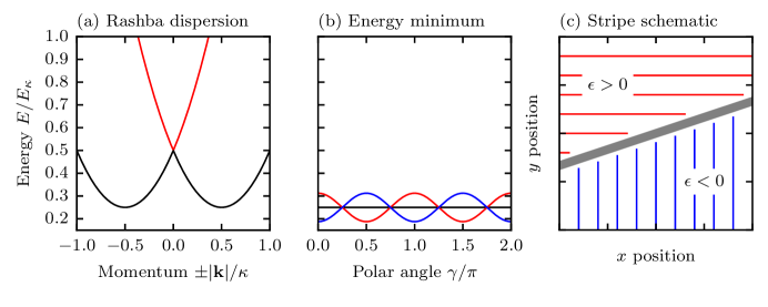
Figure 1: Spin-orbit coupled dispersion relations and spatial stripe patterns. (a) Pure Rashba dispersion plotted along the radial direction $|\bi{k}|/\kappa$. (b) Energy at the radial minima of the SOC dispersion (i.e., $|\bi{k}|/\kappa\approx 1/2$) plotted as a function of the polar angle $\gamma$ for $\epsilon=1/8$ (red), $\epsilon=0$ (black), and $\epsilon=-1/8$ (blue). (c) Representative stripe pattern showing mismatched stripe periods as projected onto the domain boundary, resulting from equal period stripes aligned along $\bi{e}_{x}$ and $\bi{e}_{y}$.

Under many realistic physical conditions, a SOBEC will Bose-condense into both of these minima simultaneously [18, 23], and the spatial interference between these two states, differing in momentum by $\delta k\approx\kappa$, will generate stripes in the atomic spin density with spatial period $2\pi/\kappa$. These stripes are aligned parallel to $\bi{e}_{x}$ for $\epsilon>0$ and parallel to $\bi{e}_{y}$ for $\epsilon<0$.

Here we study physical systems where the magnitude of the Dresselhaus SOC $\kappa\epsilon$ varies linearly along a direction in the $\bi{e}_{x}$ - $\bi{e}_{y}$ plane defined by the unit vector $\bi{e}=\cos\theta\bi{e}_{x}+\sin\theta\bi{e}_{y}$. In the half-plane with $\epsilon>0$ we expect horizontal stripes and in the half-plane with $\epsilon<0$ we expect vertical stripes (schematically shown in Fig. 1c), and we ask: how are these different patterns of stripes linked at the boundary line $0=x\cos\theta+y\sin\theta$ delineating the two domains (grey line in Fig. 1c). This seemingly simple question is nontrivial because the horizontal stripes ($\epsilon>0$) have period $d_{+}=|2\pi/\kappa\sin\theta|$ projected onto the delineating line, while vertical stripes ($\epsilon<0$) have period $d_{-}=|2\pi/\kappa\cos\theta|$ along the delineating line (see Fig. 1c): when $|\cos\theta|\neq|\sin\theta|$ stripes must terminate or originate at the domain boundary, leading to the formation of pinned topological defects.

3 Position-dependent SOC

3.1 The electronic Hamiltonian and its eigenstates

Figure 2: Proposed four level coupling scheme. (a) Coupling diagram showing our four cyclically coupled internal atomic states. (b) Spatial geometry of the coupling laser beams driving the two-photon Raman transitions. (c) Realization of the closed loop scheme in ${}^{87}\mathrm{Rb}$ using Raman transitions between magnetic sub-levels of the $f=1$ and $f=2$ hyperfine manifolds. Here $\hbar\delta=g_{F}\mu_{B}B_{0}$ is the detuning of the atomic levels $|2\rangle$ and $|4\rangle$ from two-photon Raman resonance due to an inhomogeneous magnetic field. Each line or curve connecting the bare states depicts a two-photon Raman transition.

Our inhomogeneous SOC may be created using any atom with four internal ground (or metastable) states $\{|1\rangle,|2\rangle,|3\rangle,|4\rangle\}$ that can be coupled in the cyclic manner shown in Fig. 2a. In ${}^{87}\mathrm{Rb}$ these might be the four ground hyperfine states [5] illustrated in Fig. 2c: $|{f=1,m_{F}=0,-1}\rangle$ and $|{f=2,m_{F}=0,+1}\rangle$. In that case the four states are Raman coupled with the position-dependent couplings

$$\tilde{\Omega}_{j}=\Omega_{j}\exp\left\{i[(\bi{k}_{j+1}-\bi{k}_{j})\cdot\bi{r}-\phi_{j}]\right\}$$ (2)

with amplitude $\Omega_{j}$, recoil momentum $\bi{k}_{j+1}-\bi{k}_{j}$ and phase shift $\phi_{j}$. Here

$$\bi{k}_{j}=\kappa\{\bi{e}_{x}\cos(\pi j/2)+\bi{e}_{y}\sin(\pi j/2)\}\,,\quad\,j=1,2,3,4,$$ (3)

is the wave-vector of the $j^{\mathrm{th}}$ Raman laser field, $\kappa$ being its length. This coupling scheme can be realized using the combination of $\pi$ and $\sigma$ polarized laser fields laid out in Ref. [5]. The linear Zeeman shift, from a biasing magnetic field $\bi{B}_{0}=B_{0}\bi{e}_{z}$, is rendered position-dependent by virtue of an additional magnetic field gradient $\bi{B}^{\prime}=B^{\prime}(\bi{r}\cdot\bi{e})\bi{e}_{z}$, linearly varying in the $\bi{e}_{x}$ - $\bi{e}_{y}$ plane along the direction $\bi{e}=\cos\theta\bi{e}_{x}+\sin\theta\bi{e}_{y}$. The combination $\bi{B}_{0}+\bi{B}^{\prime}$ provides a controllable detuning $\delta=\delta_{0}+\delta^{\prime}(\bi{r}\cdot\bi{e})$ from Raman resonance to the states $|2\rangle$ and $|4\rangle$, see Fig. 2c. Physically this can be realized by using atomic magnetic levels shown in Fig. 2c where one pair of states is field insensitive and the other pair share essentially the same $E_{\mathrm{Z}}=g_{F}\mu_{\mathrm{B}}|{\bf B}|m_{F}$ Zeeman shift, where $\mu_{\mathrm{B}}$ is the Bohr magneton and $g_{F}$ is the Landé g-factor (opposite in sign for the $f=1$ and $f=2$ mailfolds).

The scheme of cyclically coupled states, shown in Fig. 2, is formally equivalent to a four-site lattice with periodic boundary conditions, i.e., $|5\rangle\equiv|1\rangle$. In terms of the position-dependent states $|\tilde{j}\rangle\equiv|\tilde{j}\left(\bi{r}\right)\rangle=\exp\left(-i\bi{k}_{j}\cdot\bi{r}\right)|j\rangle$, the Hamiltonian describing the internal atomic degrees of freedom is

$$\frac{\hat{H}_{e}}{\hbar}=\tilde{\delta}I+\sum_{j=1}^{4}\tilde{\delta}(-1)^{j}|\tilde{j}\rangle\langle\tilde{j}|-\sum_{j=1}^{4}\left[\Omega_{j}e^{-i\phi_{j}}|\tilde{j}\rangle\langle\widetilde{j+1}|+\mathrm{H.c.}\right]\,.$$ (4)

where the contribution from the atom-light detuning is represented in terms of the overall shift of the energy zero $\tilde{\delta}I$ and an alternating detuning $\tilde{\delta}(-1)^{j}$, where $\tilde{\delta}=\delta/2$. This corresponds exactly to the experimental situation illustrated in Fig. 2c, where the levels $|{2}\rangle$ and $|{4}\rangle$ are shifted by $2\tilde{\delta}$, whereas the levels $|{1}\rangle$ and $|{3}\rangle$ are unaffected. Because $\tilde{\delta}$ depends on position, the energy offset $\tilde{\delta}$ cannot be removed by globally shifting the zero of energy, as in Ref. [5]. Instead the local energy shift from $\tilde{\delta}(\bi{r})$ is implicitly incorporated into the trapping potential $V(r)$ featured in Eq. (16): our linearly varying detuning simply shifts the location of the harmonic potential’s minimum.

The phases of the laser fields are taken such that $\sum_{j}\phi_{j}=\pi$, implying that an atom acquires a $\pi$ phase shift upon traversing the closed-loop $|1\rangle\rightarrow|2\rangle\rightarrow|3\rangle\rightarrow|4\rangle\rightarrow|1\rangle$ in state space. For zero detuning ($\tilde{\delta}=0$) and equal Rabi frequencies ($\Omega_{j}=\Omega$) the eigenfunctions and corresponding eigenvalues are

$$|{\chi_{q}}\rangle=\frac{1}{2}\sum_{p=1}^{4}\rme^{i\pi qp/2}|\tilde{p}\rangle\,,\quad\mathrm{and}\quad\varepsilon_{q}=-2\Omega\cos\left[\frac{\pi}{2}\left(q-\frac{1}{2}\right)\right]\,,\quad\mathrm{with}\quad q\in\left\{0,\ldots,3\right\}\,.$$ (5)

In the $\left\{|{\chi_{q}}\rangle\right\}$ basis, the internal Hamiltonian

$$\frac{\hat{H}_{e}}{\hbar}=\sum_{q=0}^{3}\varepsilon_{q}|\chi_{q}\rangle\langle\chi_{q}|+\tilde{\delta}\sum_{q=0}^{3}|\chi_{q}\rangle\langle\chi_{q-2}|$$ (6)

has two pairs of degenerate eigenstates

$$|\downarrow,\pm\rangle=a_{\mp}|\chi_{0}\rangle\pm a_{\pm}|\chi_{2}\rangle\,,\quad\mathrm{and}\quad|\uparrow,\pm\rangle=a_{\mp}|\chi_{1}\rangle\pm a_{\pm}|\chi_{3}\rangle\,,$$ (7)

labeled by the pseudospin index $\uparrow,\downarrow$ and by their energies $\pm\hbar\sqrt{\tilde{\delta}^{2}+2\Omega^{2}}$, where

$$a_{\pm}=\sqrt{\frac{1}{2}\pm\frac{\sqrt{2}\Omega}{2\sqrt{\tilde{\delta}^{2}+2\Omega^{2}}}}\,.$$ (8)

3.2 Adiabatic motion and spin-orbit coupling

We are interested in the situation where the separation energy $2\hbar\sqrt{\tilde{\delta}^{2}+2\Omega^{2}}$ between the pairs of dressed states greatly exceeds the kinetic energy of the atomic motion. In that case the atoms adiabatically move about within each two-fold degenerate manifold of pseudospin states. Such adiabatic motion is affected by the matrix-valued geometric vector and scalar potentials $\bi{A}^{(\pm)}$ and $\Phi^{(\pm)}$ which result from the position-dependence of the atomic internal dressed states [6, 12]. Here the $\pm$ signs denote to the ground or excited adiabatic manifold. The matrix elements of the gauge potentials are

$$\bi{A}^{(\pm)}_{s,s^{\prime}}=i\hbar\langle{s,\pm}|\boldsymbol{\nabla}|{s^{\prime},\pm}\rangle\,,\quad\mathrm{and}\quad\Phi^{(\pm)}_{s,s^{\prime}}=-\frac{\hbar^{2}}{2m}\sum_{s^{\prime\prime}=\uparrow,\downarrow}\langle{s,\pm}|\boldsymbol{\nabla}|{s^{\prime\prime},\mp}\rangle\langle{s^{\prime\prime},\mp}|\boldsymbol{\nabla}|{s^{\prime},\pm}\rangle\,,$$ (9)

where $s,s^{\prime}\in\left\{\uparrow,\downarrow\right\}$. Using Eq. (7) for the dressed states $\left|\uparrow,\downarrow;-\right\rangle$, one arrives at the explicit result for the gauge potentials in the ground-state manifold

$$\bi{A}^{(-)}=\frac{\hbar\kappa}{2}\left[\left(1-\epsilon\right)\sigma^{x}\bi{e}_{x}-\left(1+\epsilon\right)\sigma^{y}\bi{e}_{y}\right]\,,$$ (10)

$${\Phi^{(-)}=\frac{\hbar^{2}}{4m}\eta\left[\kappa^{2}+\eta\frac{(\boldsymbol{\nabla}\tilde{\delta})^{2}}{4\Omega^{2}}\right]I\,,}$$ (11)

with

$$\epsilon=2a_{+}a_{-}=\frac{\tilde{\delta}}{\sqrt{\tilde{\delta}^{2}+2\Omega^{2}}}\,,\quad\mathrm{and}\quad\eta=\left(a_{+}^{2}-a_{-}^{2}\right)^{2}=\frac{1}{1+\tilde{\delta}^{2}/2\Omega^{2}}\,.$$ (12)

Since the detuning $\tilde{\delta}$ varies slowly over the optical wavelength, the spatial derivatives of the detuning can be neglected in Eq. (11), giving

$$\Phi^{(-)}=\eta\frac{\hbar^{2}\kappa^{2}}{4m}I\,.$$ (13)

When the detuning is much smaller than the Rabi frequency, $\tilde{\delta}\ll\Omega$, the lowest order in $\tilde{\delta}$ contribution to the gauge potentials $\bi{A}\equiv\bi{A}^{(-)}$ and $\Phi\equiv\Phi^{(-)}$ are linear and quadratic respectively,

$$\bi{A}\approx\frac{\hbar\kappa}{2}\left[\left(1-\frac{1}{\sqrt{2}}\frac{\tilde{\delta}}{\Omega}\right)\sigma^{x}\bi{e}_{x}-\left(1+\frac{1}{\sqrt{2}}\frac{\tilde{\delta}}{\Omega}\right)\sigma^{y}\bi{e}_{y}\right]\,,$$ (14)

$$\Phi\approx\frac{\hbar^{2}\kappa^{2}}{4m}\left(1-\frac{\tilde{\delta}^{2}}{2\Omega^{2}}\right)I\,.$$ (15)

The effective scalar potential $\Phi$, resulting from the adiabatic elimination of the excited states, is proportional to the unit matrix and hence provides only an additional state-independent trapping potential.

The matrix-valued vector potential can be equivalently understood as SOC with spatially-dependence appearing via the position dependent detuning $\tilde{\delta}\equiv\tilde{\delta}\left(\bi{r}\right)$. For zero detuning, the vector potential is proportional to $\sigma^{x}\bi{e}_{x}-\sigma^{y}\bi{e}_{y}$, so the SOC is cylindrically symmetric. For non-zero detuning the cylindrical symmetry is lost, leading to the formation of the stripe phases in the SOC BEC along $\bi{e}_{x}$ or $\bi{e}_{y}$ as was discussed in Sec. 2.

4 BEC with position-dependent SOC

4.1 Equations of motion

Having now shown how to create inhomogeneous SOC, we shift our focus to its effects on ground state properties of BECs. At zero temperature, the mean-field energy functional of a spin-1/2 BEC with SOC is

$$E\left[\boldsymbol{\Psi}^{*},\boldsymbol{\Psi}\right]=\int\rmd\bi{r}\bigg{[}\Psi^{*}\frac{\left(\bi{p}-\bi{A}\right)^{2}}{2m}\Psi+V\left(r\right)\left|\Psi\right|^{2}+\Phi\left(\bi{r}\right)\left|\Psi\right|^{2}+\frac{g}{2}\left|\Psi\right|^{4}-\mu\left|\Psi\right|^{2}\bigg{]}\,,$$ (16)

where $\boldsymbol{\Psi}=\left(\psi_{\downarrow},\psi_{\uparrow}\right)^{\mathit{T}}$ is the spinor (vectorial) order parameter, $V\left(r\right)=m\omega^{2}r^{2}/2$ is the trapping potential and $g$ is the nonlinear interaction strength. The synthetic vector and scalar gauge potentials $\bi{A}$ and $\Phi$ [Eqs. (10), (13)] depend on the linearly varying detuning

$$\tilde{\delta}=\tilde{\delta}^{\prime}\left(x\cos\theta+y\sin\theta\right)$$ (17)

introduced in Sec. 3.1. Here we assume that $V(\bi{r})$ embodies all external potentials including that resulting from the spatially-dependent energy offset in Eq. (4).

The spinor time-dependent GPE (TDGPE) can be derived via the Hartree variational principle $i\hbar\partial_{t}\psi_{j}=\delta E/\delta\psi_{j}^{*}$ giving

$$i\hbar\partial_{t}\psi_{s} =\sum_{s^{\prime}}\bigg{\{}\left[-\frac{\hbar^{2}\nabla^{2}}{2m}+V+\Phi+g\rho+\frac{\left|\bi{A}\right|^{2}}{2m}-\mu\right]I_{s,s^{\prime}}$$ (18)

$$+i\frac{\hbar^{2}\kappa}{2m}\left[\left(A_{x}\partial_{x}+\frac{\partial_{x}A_{x}}{2}\right)\sigma_{s,s^{\prime}}^{x}+\left(A_{y}\partial_{y}+\frac{\partial_{y}A_{y}}{2}\right)\sigma_{s,s^{\prime}}^{y}\right]\bigg{\}}\psi_{s^{\prime}}$$

where $\rho=|\psi_{\downarrow}|^{2}+|\psi_{\uparrow}|^{2}$ is the total density. Equation (18) governs the dynamics of the BECs with position-dependent SOC, at the mean-field level.

4.2 Ground-state phases of the SOBEC

In Sec. 2, we discussed the single particle properties expected in our mixed Rashba-Dresselhaus spin-orbit coupled system and noted that when $\epsilon\neq 0$ the spectrum is two-fold degenerate at points $\bi{k}_{\pm}/\kappa=\pm(1+\epsilon)\bi{e}_{y}/2$ for $\epsilon>0$ and $\bi{k}_{\pm}/\kappa=\pm(1-\epsilon)\bi{e}_{x}/2$ for $\epsilon<0$. When weak repulsive interactions are included, the bosons can condense either in: (1) a plane-wave phase (PW) in which one of $\bi{k}_{+}$ or $\bi{k}_{-}$ is macroscopically occupied; or in (2) a standing wave phase (SW, sometimes called a striped phase) in which the bosons condense into a coherent superposition of $\bi{k}_{+}$ and $\bi{k}_{-}$. We focus on the case where the inter- and intra- spin interactions are identical, for which the ground state is in the SW phase [18, 23].

The detuning $\tilde{\delta}$ vanishes along the separatrix $x\cos\theta+y\sin\theta=0$ that delineates the regions with $\tilde{\delta}>0$ and $\tilde{\delta}<0$. Since the wave vectors characterizing the two domains have differing projections onto the line where $\tilde{\delta}=0$, novel structures can form to heal the otherwise discontinuous strip patterns at opposite sides of the separatrix. For example, for $\tan\theta=1$ and $2$, we expect one-to one and two-to-one connections on the interface, respectively.

We determined the ground state of the SOBEC – minimizing the energy functional in Eq. (16) – by propagating Eq. (18) with differing degrees of imaginary time [24, 25, 26, 27]: replacing $i\partial_{t}$ by $i\exp[i\zeta]\partial_{t}$ in Eq. (18), for $\zeta\in[0,\pi/2]$. While simulations converged to the same solution for any non-negligible $\zeta$, the resulting damped GPE converges much more rapidly for proper choice of $\zeta$. We confirmed that obtained the ground state by the absence of any time-dependance when we evolve in real time. We considered a 2D ${}^{87}\mathrm{Rb}$ BEC confined in a harmonic potential with frequency $\omega/2\pi=100\,\mathrm{Hz}$. For computational convenience, we adopt the dimensionless units where the frequency and length are scaled in units of the trap frequency $\omega/2\pi$ and the oscillator length $\sqrt{\hbar/m\omega}$, respectively. We employ the Fourier pseudospectral method with $N_{x}=N_{y}=256$ grid points.

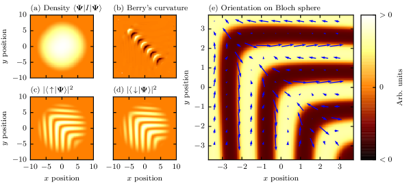
Figure 3: The ground state of a spatially dependent SOC BEC with a commensurate interface. This simulation was performed with $\mu=32\hbar\omega$, $\tilde{\delta}^{\prime}=\Omega/2$, $\kappa=2$, and $\theta=\pi/4$. (a)–(d) plot the density $\langle{\boldsymbol{\Psi}}|I|{\boldsymbol{\Psi}}\rangle$, the Berry’s curvature ${\mathcal{B}}_{z}$, and the densities in the spin up and spin down components $|\left<\uparrow\!|\boldsymbol{\Psi}\right>|^{2}$, and $|\left<\downarrow\!|\boldsymbol{\Psi}\right>|^{2}$. Each of these quantities varies smoothly across the domain interface, continuously connecting the the two SW phases. (e) Orientation of the local spin vector on the Bloch sphere. The colored background gives the $\bi{e}_{z}$ component, while the vector field plots the $\bi{e}_{x}$ and $\bi{e}_{y}$ components.

We first consider the parameters $\tilde{\delta}^{\prime}=\Omega/2$, $\kappa=2$, $\theta=\pi/4$, and $\mu=32\hbar\omega$ which corresponds to $gN_{\uparrow}=gN_{\downarrow}\simeq 1500$. In this case $\cos\theta=\sin\theta$ and the horizontal and vertical stripes are matched one-to-one at the boundary. The corresponding ground-state wave function is shown in Fig. 3. In this case, the interface lies along the line $x+y=0$ and the stripes align along $\bi{e}_{y}$ for $x+y<0$ and along $\bi{e}_{x}$ for $x+y>0$. Clearly, the stripes in both domains are connected one-to-one across the interface. Moreover, the orientation of the state along the Bloch sphere smoothly connects the two phases, as shown in Figs. 3e. The ground-state structure is consistent with the prediction of the noninteracting homogeneous system with our single particle arguments.

These stripes are associated with the local spin vector

$${\bf N}=\langle{\boldsymbol{\Psi}}|{\boldsymbol{\sigma}}|{\boldsymbol{\Psi}}\rangle\,,\quad{\rm and\ orientation}\quad{\bf n}=\frac{{\bf N}}{|{\bf N}|}$$ (19)

precessing on the Bloch sphere (Fig. 3e) either in the $\bi{e}_{x}$-$\bi{e}_{z}$ plane (horizontal stripes) or the $\bi{e}_{y}$-$\bi{e}_{z}$ plane (vertical stripes). The changing orientation in these precession planes leads to a chain of vortices in the spin degree of freedom: distorted skyrmions and anti-skyrmions. We quantify the location of these vortices in Fig. 3b where we plot the local Berry’s curvature

$${\mathcal{B}}_{z} =-\frac{\hbar}{2}\left(\frac{\partial_{x}n_{x}\partial_{y}n_{y}-\partial_{y}n_{x}\partial_{x}n_{y}}{n_{z}}\right)$$ (20)

which is peaked at the vortex centers. This clearly shows the ordered chain of skyrmions at the stripe-interface.

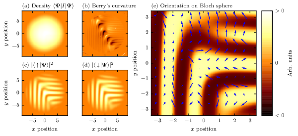
Figure 4: The ground state of a spatially dependent SOC BEC with an incommensurate interface. This simulation was performed with $\mu=32\hbar\omega$, $\tilde{\delta}^{\prime}=\Omega\sqrt{10}/6$, $\kappa=2$ and $\tan\theta=1/2$. (a)–(d) plot the density $\langle{\boldsymbol{\Psi}}|I|{\boldsymbol{\Psi}}\rangle$, the Berry’s curvature ${\mathcal{B}}_{z}$, and the densities in the spin up and spin down components $|\left<\uparrow\!|\boldsymbol{\Psi}\right>|^{2}$, and $|\left<\downarrow\!|\boldsymbol{\Psi}\right>|^{2}$. Because the projection of the stripe periods along the interface are mismatched, defects form at the domain interface between the two SW phases. (e) Orientation of the local spin vector on the Bloch sphere. The colored background gives the $\bi{e}_{z}$ component, while the vector field plots the $\bi{e}_{x}$ and $\bi{e}_{y}$ components.

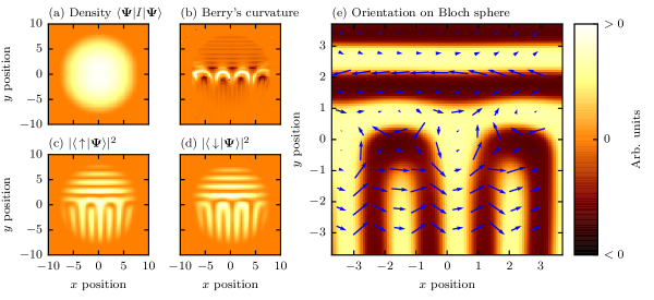
Figure 5: The ground state of a spatially dependent SOC BEC with orthogonal stripe patterns. This simulation was performed with $\mu=32\hbar\omega$, $\tilde{\delta}^{\prime}=\Omega/\sqrt{2}$, $\kappa=2$ and $\theta=\pi/2$. In this case, the boundary occurs at $x=0$. Panels (a)–(d) plot the density $\langle{\boldsymbol{\Psi}}|I|{\boldsymbol{\Psi}}\rangle$, the Berry’s curvature ${\mathcal{B}}_{z}$, and the densities in the spin up and spin down components $|\left<\uparrow\!|\boldsymbol{\Psi}\right>|^{2}$, and $|\left<\downarrow\!|\boldsymbol{\Psi}\right>|^{2}$. A row of vortices forms to link the two completely incompatible SW patterns. (e) Orientation of the local spin vector on the Bloch sphere. The colored background gives the $\bi{e}_{z}$ component, while the vector field plots the $\bi{e}_{x}$ and $\bi{e}_{y}$ components.

Next we investigate how the ground-state density and phase profiles vary over the interface region for the mismatched condition when two stripes in one domain are linked to a single stripe in the other. Specifically, we consider $\tan\theta=1/2$ and $\tilde{\delta}^{\prime}=\Omega\sqrt{10}/6$, which gives a separatrix $2x+y=0$. Keeping the same values of $\mu$, $\kappa$ we used for $\theta=\pi/4$ case, the ground state is shown in Fig. 4. We observe that, near the trap center, every two adjacent stripes in the region of $2x+y>0$ connect to one single stripe in the region of $2x+y<0$. Unlike the previous case with $\theta=\pi/4$, where the density and phase profiles both vary smoothly across the interface, in the current case the phases profile does not vary smoothly across the interface. In the spin-projections shown in Fig. 4e we see that vortices form at the boundary. In this case, two stripes must merge—and also form an excess vortex—before a single stripe crosses the domain boundary. The existence of an imbalanced number vortices in the ground state results from the merging of stripes, and is clearly visible in the Berry’s curvature (Fig. 4b) which now favors negative values at the interface. In conventional BECs, vortices are stabilized by the application of artificial magnetic fields. However in our spatially dependent SOC BEC, the ground state supports vortices at the interface between two distinct SW phases. Similar defect formation at the interface of two distinct ground state phases was studied for spin-1 BECs with tunable inter- and intra- species interactions [28, 29].

Finally we examine the case where $\theta=\pi/2$ and $\tilde{\delta}^{\prime}=\Omega/\sqrt{2}$: here the interface coincides with the $x$-axis. In this case the stripes for $y<0$ are perpendicular to the interface while the stripes are parallel to the interface in the region of $y>0$. The result is shown in Fig. 5. The orthogonal stripes result in the formation of a vortex chain on the interface that can be seen clearly in the spin-projections of Fig. 5e and in the Berry’s curvature in Fig. 5b. Our results indicate that the unconventional BEC ground state contains chains of vortices and anti-vortices stabilized by the position-dependent SOC. Furthermore, the number of vortices is highly controllable by tuning the size of condensate, the spin-orbit coupling strength $\kappa$, and the orientation of the interface.

5 Concluding remarks

We proposed a new technique for creating position-dependent SOC for cold atomic BECs. This can be implemented by combining a cyclic Raman coupling scheme [5] to induce SOC, along with a magnetic field gradient [30, 31] to impart a spatial dependance.

Subject to this combination, we find that a weakly interacting BEC phase separates into two domains with orthogonally oriented stripes. Depending on axes of the domain boundary—set by the spatial direction of the magnetic field gradient—the stripes from each domain can intersect the boundary with matched or mismatched spatial periods. We show that when the stripe patterns intersect with different spatial periods, a chain of topological defects, including vortices and anti-vortices, form to link the mismatched stripe patterns. In contrast to vortices present in conventional rotating BECs, here the vortices are stable topological defects that are not present in the homogenous phase (here the SW phase). These vortices can form in an ordered chain when the relative periods at the domain wall are different, but commensurate, and they form a disordered chain when the relative periods are incommensurate.

References

References

- [1] Ruseckas J, Juzeliūnas G, Öhberg P and Fleischhauer M 2005 Phys. Rev. Lett. 95 010404
- [2] Stanescu T D, Zhang C and Galitski V 2007 Phys. Rev. Lett. 99 110403
- [3] Jacob A, Öhberg P, Juzeliūnas G and Santos L 2007 Appl. Phys. B 89 439
- [4] Juzeliūnas G, Ruseckas J, Lindberg M, Santos L and Öhberg P 2008 Phys. Rev. A 77 011802(R)
- [5] Campbell D L, Juzeliūnas G and Spielman I B 2011 Phys. Rev. A 84 025602
- [6] Dalibard J, Gerbier F, Juzeliūnas G and Öhberg P 2011 Rev. Mod. Phys. 83 1523–1543
- [7] Anderson B M, Juzeliūnas G, Galitski V M and Spielman I B 2012 Phys. Rev. Lett. 108 235301
- [8] Zhai H 2012 Int. J. Mod. Phys. B 26 1230001
- [9] Galitski V and Spielman I B 2013 Nature 494 49–54
- [10] Liu X J, Law K T and Ng T K 2014 Phys. Rev. Lett 112 086401
- [11] Zhai H 2015 Rep. Prog. Phys. 78 026001
- [12] Goldman N, Juzeliūnas G, Öhberg P and Spielman I B 2014 Rep. Progr. Phys. 77 126401
- [13] Anderson B M, Spielman I B and Juzeliūnas G 2013 Phys. Rev. Lett. 111 125301
- [14] Xu Z F, You L and Ueda M 2013 Phys. Rev. A 87 063634
- [15] Stanescu T D, Anderson B and Galitski V 2008 Phys. Rev. A 78 023616
- [16] Cong-Jun W, Mondragon-Shem I and Xiang-Fa Z 2011 Chinese Phys. Lett. 28 097102
- [17] Sinha S, Nath R and Santos L 2011 Phys. Rev. Lett. 107 270401
- [18] Wang C, Gao C, Jian C M and Zhai H 2010 Phys. Rev. Lett. 105 160403
- [19] Vyasanakere J P and Shenoy V B 2011 Phys. Rev. B 83 94515
- [20] Vyasanakere J P, Zhang S and Shenoy V B 2011 Phys. Rev. B 84 14512
- [21] Yu Z Q and Zhai H 2011 Phys. Rev. Lett. 107 195305
- [22] Jiang L, Liu X J, Hu H and Pu H 2011 Phys. Rev. A 84 063618
- [23] Xu Z F, Lu R and You L 2011 Phys. Rev. A 83 053602
- [24] Choi S, Morgan S A and Burnett K 1998 Phys. Rev. A 57 4057
- [25] Penckwitt A A, Ballagh R J and Gardiner C W 2002 Phys. Rev. Lett. 89 260402
- [26] Tsubota M, Kasamatsu K and Ueda M 2002 Phys. Rev. A 65 023603
- [27] Billam T P, Reeves M T, Anderson B P and Bradley A S 2014 Phys. Rev. Lett. 112 145301
- [28] Borgh M O and Ruostekoski J 2012 Phys. Rev. Lett. 109 015302
- [29] Borgh M O and Ruostekoski J 2013 Phys. Rev. A 87 033617
- [30] Spielman I B 2009 Physical Review A (Atomic, Molecular, and Optical Physics) 79 063613
- [31] Lin Y J, Compton R L, Jim enez-Garc i a K, Porto J V and Spielman I B 2009 Nature 462 628–632