Cross-Modal Learning via Pairwise Constraints

Abstract

In multimedia applications, the text and image components in a web document form a pairwise constraint that potentially indicates the same semantic concept. This paper studies cross-modal learning via the pairwise constraint, and aims to find the common structure hidden in different modalities. We first propose a compound regularization framework to deal with the pairwise constraint, which can be used as a general platform for developing cross-modal algorithms. For unsupervised learning, we propose a cross-modal subspace clustering method to learn a common structure for different modalities. For supervised learning, to reduce the semantic gap and the outliers in pairwise constraints, we propose a cross-modal matching method based on compound $\ell_{21}$ regularization along with an iteratively reweighted algorithm to find the global optimum. Extensive experiments demonstrate the benefits of joint text and image modeling with semantically induced pairwise constraints, and show that the proposed cross-modal methods can further reduce the semantic gap between different modalities and improve the clustering/retrieval accuracy.

I Introduction

Multimedia information of data presents diversified combination of different forms, such as text, video, still images, and live TV. It is intrinsically multi modal [1] and often requires a web document corpus with paired text and images (or other forms). One of its fundamental tasks is to learn cross-modal information from multiple content modalities. Recently, the terms ’cross-modal’[2][3], ’multi-modal’[1][4] and ’multi-view’[5][6] are all used for multimedia information processing, and the word ’modality’ has different interpretation in different applications. In this paper, multiple modalities (e.g., text and images) are assumed to have a loose relation, and each modality, which gives a different aspect of multimedia information, has a dependent relationship to other modalities [1].

In multimedia information processing, one popular strategy is to apply paired samples from different modalities to learn a common latent structure (or space) and then to perform clustering or retrieval. The paired samples refer to the samples from different modalities that belong to the same semantic unit( e.g., text and image in a web document, image features and associated tags for an image) and form a pairwise constraint for different modalities as shown in Fig. 1. This pairwise constraint problem has also drawn much attention in other applications such as multi-pose face recognition [5][7], biometric verification [8], multilingual retrieval [9], semi-supervised learning [10] and dictionary learning [11][12].

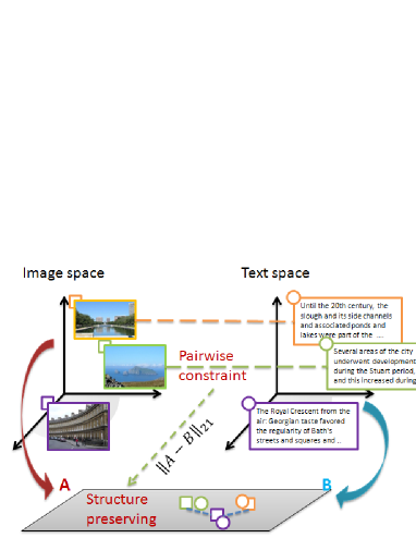
Figure 1: Cross-modal learning via pairwise constraint. (a) An example of image-text pair from the Wiki dataset [2]. The image has a loosely related text description [3]. (b) The pairwise constraint induces two basic problems: how to learn a common structure for two modalities? and how to preserve the structure during learning? Data sets A and B are the representations of two modalities respectively in a hidden space, in which paired points are close meanwhile the pairwise constraint induced structure between data points are preserved. $\ell_{21}$-norm is adpoted to improve robustness and reduce the semantic gap between low-level features and high-level concepts.

Although different methods have been developed for cross-modal learning and pairwise constraints have drawn much attention in different communities, to the best of our knowledge, there may be not any existing works to fully explore pairwise constraint problems from a unified viewpoint. In multimedia information processing, since different modalities are in one single document (e.g., the text and image in a web document as shown in Fig. 1), they form a pairwise constraint and give different aspects of multimedia information. However, as shown in Fig. 1 (a), the paired samples often have a loose relationship [3], which makes the cross-modal learning with pairwise constraints more challenging. In addition, since there is a semantic gap between low-level features and high-level concepts, the pairwise constraint often leads to two basic problems for learning methods as shown in Fig. 1 (b):

1) How to learn a common structure for two modalities? Because of the semantic gap, one can obtain different structures from different modalities. For example, points $x_{i}$ and $x_{j}$ may be neighbors in the text space whereas they are not in the image space. However, these structures must be the same neighborhood structure due to the pairwise constraint.

2) How to preserve the structure during learning? For a cross-modal learning algorithm, two modalities in the learned subspace (or representation) should satisfy the original pairwise constraint and preserve the original neighborhood structure.

This paper systematically studies the pairwise constraint and its induced structure preserving problems, and accordingly proposes a general regularization framework to find the common structure hidden in different modalities . In particular, for unsupervised learning, we propose a cross-modal subspace learning method, in which different modalities share a common structure. A simple but efficient algorithm is further developed to solve the subspace clustering problem. For supervised learning, to reduce the semantic gap and the outliers in pairwise constraints, we propose a cross-modal matching method based on compound $\ell_{21}$ regularization, which can be efficiently solved by an iteratively reweighted algorithm. At each iteration, the compound $\ell_{21}$ regularization problem is simplified to a least squares problem. Extensive experiments on several widely used databases demonstrate the benefits of joint text and image modeling with pairwise constraints.

The main contribution of this work lies in three-fold:

1) We make a systematic investigation on the pairwise constraint in cross-modal learning, and design a general regularization framework, which can be used as a general platform for developing unsupervised and supervised learning algorithms.

2) For unsupervised learning, to the best of our knowledge, it is the first time to extend the linear presentation based subspace clustering methods [13][14][15][16] to deal with the multi-modal case. Experimental results show that the clustering accuracy can be improved when multi-modal information is used.

3) For supervised learning, a $\ell_{21}$ regularization method is proposed for cross-modal matching, which can handle intra-class variation, pairwise constraint and structure preserving at the same time. It obtains the state-of-the-art results in the Wiki text-image dataset [2].

The rest of this paper is organized as follows. In Section II, we briefly review existing cross-modal (or multi-modal) learning methods. In Section III, we propose a general framework for cross-modal learning. In particular, a cross-modal subspace clustering method and a cross-modal matching method are developed for unsupervised and supervised learning respectively. Section IV provides a series of experiments to systematically evaluate the effectiveness of the proposed methods, prior to the summary of this paper in Section V.

II Related work

Our proposed unsupervised and supervised multi-modal learning methods correspond to clustering and retrieval tasks respectively. In this section, we accordingly review some related cross-modal methods in clustering and matching tasks.

II-A Clustering on multi-modal data

For clustering, Basu et al. [17] presented a pairwise constrained clustering framework together with a method to select informative pairwise constraints to improve clustering performance. Cho et al. [18] proposed a minimum sum-squared residue co-clustering method for gene expression data. Tong et al. [4] studied a graph based multi-modality clustering algorithm to group multiple modalities. Based on combinatorial Markov random field, Bekkerman and Jeon [1] developed a multi-modal clustering method for multimedia collections. Based on spectral clustering, Yogatama and Tanaka-Ishii [9] presented a multilingual spectral clustering to merge two language spaces via pairwise constraints; and by combining co-regularization for multiple views [19][10], Kumar et al. [20][21] presented co-training and co-regularized approaches for multi-view spectral clustering respectively. In addition, deep networks were used in [22][23] to learn shared representations for multi-modal data. Wang et al. [24] resorted to the cross diffusion process to fuse multiple metrics. The authors in [25][26] apply the similarity (or dissimilarity) measures w.r.t. pairwise constraints to exemplar clustering and exemplar finding tasks respectively. Base on structured sparsity, Wang et al. [27] proposed to learn cluster indication matrix and then used K-means to perform clustering. Hua and Pei [28] proposed bottom-up and top-down methods for mutual subspace clustering.

Recently, structure prior information (such as sparse [13], low-rank [14], or collaborative [16]) has shown to be effective for single-modality clustering and often results in better clustering accuracy, which drives us to develop new multi-modal clustering methods based on the structure prior information.

II-B Cross-modal matching

For retrieval, the most famous cross-modal methods to obtain a common space for multiple modalities are canonical correlation analysis (CCA) [29][2] and partial least squares (PLS) [30][31], which learn transformations to project each modality into a common space. Since CCA does not use label information of multiple modalities, multi-view discriminant analysis [32][5] are further developed to make use of label information. By means of locality preserving, Sun and Chen [33] presented locality preserving CCA, and Quadrianto and Lampert [34] developed multi-view neighborhood preserving projections. Based on bilinear models [35], Sharma et al. [36] further extended multi-view discriminant analysis to a generalized multi-view analysis in terms of graph embedding [37]. Weston et al. [38][39] tried to learn common representation spaces for images and their annotations. Sang and Xu [40] provided a new perspective of multi-modal video analysis by exploring the pairwise visual cues for constrained topic modeling. Based on structured sparsity, Zhuang et al. [41] proposed a supervised coupled dictionary learning method for multi-modal retrieval.

In other multi-modal applications, Lin and Tang [42][7] resorted to subspace learning for inter-modality face recognition. Ye et al. [43] applied pairwise relationship matrix for robust late fusion. Cui et al. [8] developed a pairwise constrained multiple metric learning method for face verification. In dictionary learning, the authors in [11][12][41] resorted to paired samples to learn discriminative dictionaries for image classification. Kulis et al. [44] proposed asymmetric kernel transforms for cross domain adaptation. Chen et al. [45] proposed a general framework to deal with semi-paired and semi-supervised multi-view data, which combines both structural information and discriminative information. By considering side information, Qian et al. [46] proposed a multi-view classification method with cross-view must-link and cannot-link constraints. Xu et al. [47] extended the theory of the information bottleneck to learn from examples represented by multi-view features. Jiang et al. [48] developed a novel semi-supervised unified latent factor learning method for partially labeled multi-view data.

Although many learning algorithms have been developed for cross-modal problems and pairwise constraints have been studied in cross-modal learning, there is still not any systematic work to fully explore pairwise constraints. Hence a general cross-modal learning framework may be potentially useful for future research.

III Cross modal learning via pairwise constraints

In this section, we study unsupervised and supervised methods for cross-modal learning via the pairwise constraint. Although the proposed ideas can also be used for multi-view learning [7][36], multi-task learning [49][50] and other combinations of content modalities [18][40], here we restrict our study to documents containing images and text as in [2][31]. The goal is to utilize the pairwise constraint to improve learning results.

III-A A general framework

Web documents often pair a body of text with a number of images [2], which form pairwise constraints for cross-modal learning. For simplicity, we only discuss the case that one document contains only one image and a body of text such that there is only one pairwise constraint in one document. Let $X_{A}\in R^{d_{A}\times n}$ and $X_{B}\in R^{d_{B}\times n}$ are two modalities of documents that contain components of images and text respectively, $n$ is the number of documents, and $d_{A}$ and $d_{B}$ are feature dimensions of images and text respectively. We expect to learn subspaces $U_{I}$ ($I\in\{A,B\}$) and their corresponding embedding $Z_{I}$ such that $U_{I}Z_{I}$ can mostly agree with $X_{I}$. In addition, due to the semantic gap between different modalities, the representation abilities of multi-modal features are imbalanced so that a unique $Z_{I}=Z$ cannot represent different modalities well. To alleviate this problem, we also expect embedding $Z_{A}$ and $Z_{B}$ are closer as much as possible according to the pairwise constraint. Hence, we have the following cross-modal learning problem in general,

$$\min_{U_{I},Z_{I}}\sum\limits_{I}(w_{I}\left\|{X_{I}-U_{I}Z_{I}}\right\|_{F}^{2}+\lambda_{1}f_{s}(U_{I},Z_{I}))$$ (1)

$$+\lambda_{2}\left\|{Z_{A}-Z_{B}}\right\|,$$

where $w_{I}$, $\lambda_{1}$ and $\lambda_{2}$ are constants, $\left\|.\right\|_{F}$ is matrix Frobenius norm, $f_{s}(.)$ is a function about $U_{I}$ and $Z_{I}$ to preserve the structure, and $\left\|.\right\|$ is a potential norm to handle the property of $Z_{A}-Z_{B}$, e.g., $\ell_{1}$-norm, $\ell_{21}$-norm or nuclear norm. The minimization problem in (1) is non-convex w.r.t $\{U_{I},Z_{I}\}$. When $U_{I}$ or $Z_{I}$ is fixed, (1) becomes the co-regularized least squares regression problem [51][52][53]; and if $\ell_{1}$-norm is used in $\left\|{Z_{A}-Z_{B}}\right\|$, (1) can be viewed as an extension of the pairwise lasso problem [10][54].

The first item in (1) is a data adaptation item, the second item controls the complexity of subspace $U_{I}$, and the last one models the pairwise constraint between two modalities. Both the second and third items facilitate structure preserving. For example, $f_{s}(.)$ and $\left\|.\right\|$ on ${U_{I}}$ can be nuclear norm, structured sparsity induced norm, or a graph Laplacian regularization in Subsection III-C. The second item aims to preserve the structure of each modality and the third item ensures that the structures of different modalities are similar. For unsupervised learning, $U_{I}$ can be a dictionary to express modality $X_{I}$, and $Z_{I}$ can be graph affinity matrix for each modality [4][20][21]; and for supervised learning, $U_{I}$ can be a discriminative projection matrix to project different modalities into a common subspace for cross-modal retrieval/classification, and $Z_{I}$ can be a group indicator matrix to represent different semantic groups [36][5]. In addition, (1) can be viewed as a dictionary learning problem with paired samples in [11][12], in which $U_{I}$ and $Z_{I}$ are a dictionary and a coefficient matrix respectively. In the following two subsections, we will detail the proposed model in (1) for unsupervised learning and supervised learning respectively.

III-B Unsupervised learning

Clustering is one of main components in multimedia management systems. For multimedia information, an effective clustering system aims to handle complex structures and discover common representations of multimedia documents [1]. Here, we focus on the problem of bridging multi-modal spaces for web document clustering. We are given web documents with different modalities (e.g., text and image) and asked to group them into clusters so that web documents from the same topic are grouped together.

Inspired by the recent advances in subspace clustering (or segmentation) [13], we consider a diagonal constraint $diag(Z_{I})=0$ and set subspace $U_{I}$ to be $X_{I}$. In addition, we expect that $Z_{I}$ can reflect some data structures, such as sparse and low-rank. Hence we let $f_{s}(U_{I},Z_{I})=\left\|{Z_{I}}\right\|$ that is a structure preserving item to make $Z_{I}$ be collaborative, sparse or low-rank as in subspace clustering [13][14]. Then (1) takes the following form,

$$\min_{Z_{I}}\sum\limits_{I}{(w_{I}\left\|{X_{I}-X_{I}Z_{I}}\right\|_{F}^{2}+\lambda_{1}\left\|{Z_{I}}\right\|)}+\lambda_{2}\left\|{Z_{A}-Z_{B}}\right\|,$$ (2)

where $Z_{I}$ indicates a graph affinity matrix for each modality as in [4][20][21] (That is, one modality is represented as one independent graph [4]). The last item $\left\|{Z_{A}^{T}-Z_{B}^{T}}\right\|$ makes each graph $Z_{I}$ to agree with each other under the constraint formulated by a norm $\left\|.\right\|$, such as $\ell_{1}$, $\ell_{2}$ and nuclear norms. Here we consider a simple case of $\ell_{2}$-norm. Then we have,

$$\min_{Z_{I}}\sum\limits_{I}{(w_{I}\left\|{X_{I}-X_{I}Z_{I}}\right\|_{F}^{2}+\lambda_{1}\left\|{Z_{I}}\right\|_{F}^{2})}+\lambda_{2}\left\|{Z_{A}-Z_{B}}\right\|_{F}^{2}.$$ (3)

Furthermore, let $Z=(Z_{A}+Z_{B})/2$, we can derive that,

$$Z_{A}-Z_{B}=2Z_{A}-(Z_{B}+Z_{A})=2Z_{A}-2Z.$$

Hence (3) can be reformulated as,

$$\min_{Z_{I},Z}\sum\limits_{I}{(w_{I}\left\|{X_{I}-X_{I}Z_{I}}\right\|_{F}^{2}+\lambda_{1}\left\|{Z_{I}}\right\|_{F}^{2}+\lambda_{3}\left\|{Z_{I}-Z}\right\|_{F}^{2})},$$ (4)

where $\lambda_{3}=2\lambda_{2}$.

If we set the derivative of (4) with respect to $Z$ equal to zeros, we obtain that the optimal solution of $Z$ takes the form,

$$Z^{*}=(Z_{A}^{*}+Z_{B}^{*})/2,$$ (5)

where $Z_{A}^{*}$ and $Z_{B}^{*}$ are optimal solutions of $Z_{A}$ and $Z_{B}$ respectively.

The optimal solution of (4) can be obtained in an alternating minimization way. We can set the derivative of (4) with respect to $Z_{I}$ equal to zeros respectively and find a solution of $Z_{I}$. Considering that the diagonal constraint $diag(Z_{I})=0$ in subspace clustering, we can compute $Z_{I}$ as follows,

$$z_{i}^{I}=(w_{I}\bar{X}_{I}^{T}\bar{X}_{I}+\lambda_{1}I+\lambda_{3}I)^{-1}(w_{I}\bar{X}_{I}^{T}x_{i}^{I}+\lambda_{3}z_{i}^{*}),$$ (6)

where $z_{i}^{I}\in{R^{\left({n-1}\right)\times 1}}$ is the $i$-th column of $Z_{I}$ excluding $Z_{I(ii)}=0$, $\bar{X}_{I}\in{R^{{d_{I}}\times\left({n-1}\right)}}$ indicates all data points in $X_{I}$ excluding $x_{i}^{I}$, $x_{i}^{I}$ indicates the $i$-th data point in $X_{I}$, and $z_{i}^{*}$ is the $i$-th column of $Z$ excluding $Z_{ii}$.

Input: $X_{A}\in R^{d_{A}\times n}$, $X_{B}\in R^{d_{B}\times n}$, parameter $\lambda_{1}$ and $\lambda_{3}$, the number of clusters $c$

Output: Groups of the dataset

1:      For $i=1:n$

2:          Repeat:

3:            Solve $z_{i}^{I}$ according to (6);

4:            Solve $Z$ according to (5);

5:          Until convergence

6:      End

7:      Define the affinity matrix $A=\frac{1}{2}({\left|{{Z^{T}}}\right|}+\left|{{Z}}\right|)$.

8:  Apply the Ncuts [55] to the affinity matrix $A$.

Algorithm 1 Cross-modal Subspace Clustering (CSC) with Pairwise Constraint

Algorithm 1 summarizes the procedure of our cross-modal subspace clustering method. Since we can compute $Z$ by computing each $z^{*}_{i}$ independently, the computation of $Z$ can be separated and paralleled. To further reduce computational costs of each $z^{*}_{i}$, we can minimize (6) only from $x_{i}^{I}$’s nearest neighborhood samples. As a result, the computation mainly depends on the iteration in Algorithm 1 rather than the number of data. When the number of data tends to be large, the major computational cost of Algorithm 1 depends on its clustering step.

III-C Supervised learning

In multimedia retrieval applications, a practical cross-modal retrieval problem often includes two tasks [2]: one is to retrieve images in response to a query text; and the other is to retrieve text documents in response to a query image. Recently, some learning methods are developed to learn common representations [23][22] or discriminative subspaces [31][36][5] for cross-modal problems. Inspired by these methods, we aim to learn two subspaces $U_{A}$ and $U_{B}$ in which the projected data are most discriminative and relevant. Furthermore, we resort to the indicator matrix (or spectral matrix) $Y\in R^{n\times c}$ in linear discriminant analysis (LDA) [56][57] as the hidden space $Z$ in (1) for two modalities. Then we have the following loss function,

$$f(U_{A},U_{B})\buildrel\textstyle.\over{=}\sum\nolimits_{I}{\left\|{U_{I}^{T}X_{I}-Y}\right\|}_{F}^{2},$$ (7)

where

$$Y_{il}=\left\{{\begin{array}[]{*{20}c}1&{{\rm{if\;}}x_{i}{\rm{\;belongs\;to\;the\;}}l-{\rm{th\;class}}}\\ 0&{{\rm{otherwise}}}\\ \end{array}}\right.,$$ (8)

and $l\in\{1,\dots,c\}$. The definition of (8) is the same as (15) in [56] and (12) in [57]. Note that, for a specific application, the label matrix $Y$ can be any other spectral matrices of graph embedding methods [56]. If we only consider one modality in (7) and $Y$ is the indicator matrix of LDA, (7) becomes the least square formulation of LDA in terms of graph embedding [56], which makes use of within-class and between-class variations for a discriminative purpose. Hence, (7) can also be viewed as a natural extension from single modality LDA to multiple modalities.

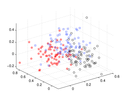
Figure 2: A three-dimensional representation of the set of Wiki image data using (7). For the first three categories, 70 image samples per category are randomly selected from the Wiki training dataset. Then (7) is applied to obtain the lower dimensional representation $U_{B}X_{B}$.

In (7), if each $U_{I}^{T}X_{I}$ is close enough to $Y$, $U_{A}^{T}X_{A}$ and $U_{B}^{T}X_{B}$ will be close to each other so that cross-modal retrieval on $X_{A}$ and $X_{B}$ will be very accurate. However, because of semantic gap between high-level semantic concept and low-level features, $U_{A}^{T}X^{A}$ and $U_{B}^{T}X^{B}$ may be not close to $Y$. In real-world cross-modal retrieval tasks, it is almost impossible to find two subspaces $U_{A}$ and $U_{B}$ so that $U_{A}^{T}X_{A}=U_{B}^{T}X_{B}=Y$. Particularly, a pair of data $U_{A}x_{i}^{A}$ and $U_{B}x_{i}^{B}$ may be far away from each other. Because (7) is a least square formation of LDA, it only facilitates clustering the data from the same class as well as making the data from different classes be far away. Fig. 2 gives an illustration on the Wiki text-image dataset. We observe that although the images from the first three categories tend to be clustered in the three dimensional subspace, each projection point $U_{B}x_{i}^{B}$ is not close to the indicator matrix $Y$.

Considering that structure preserving is often useful in graph embedding methods, we substitute $f_{s}(U_{I},Z_{I})$ in (1) with a structure preserving item, i.e., $f_{s}(U_{I},Z_{I})=\sum\nolimits_{I}{\sum\nolimits_{\{i,j\}}{w_{ij}\left\|{U_{I}^{T}(x_{i}^{I}-x_{j}^{I})}\right\|_{2}}}$. $w_{ij}$ is a constant that indicates the relationship between $x^{I}_{i}$ and $x^{I}_{j}$. Because of the semantic gap, the observed relationship between $x^{A}_{i}$ and $x^{A}_{j}$ may be different from that between $x^{B}_{i}$ and $x^{B}_{j}$. A simple way to solve this problem is to concatenate the feature vectors in each modality, and then resort to a weighting calculation strategy in graph embedding to learn a high-level relationship.

Although $f(U_{A},U_{B})$ in (7) clusters data and $f_{s}(U_{I},Z_{I})$ preserves data structure, both $f(U_{A},U_{B})$ and $f_{s}(U_{I},Z_{I})$ can not ensure each pair of modal data be close to each other in the projection subspace. Hence we need to introduce an item to make each pair of modal data follow pairwise constraints. By combining all things together, we obtain the following regularization problem via (1),

$$\mathop{\min}\limits_{U_{A},U_{B}}f(U_{A},U_{B})+\lambda_{1}\sum\limits_{I}{\sum\limits_{i,j}{w_{ij}\left\|{U_{I}^{T}(x_{i}^{I}-x_{j}^{I})}\right\|_{2}}}$$ (9)

$$+\lambda_{2}\left\|{X_{A}^{T}U_{A}-X_{B}^{T}U_{B}}\right\|_{21},$$

where $\left\|M\right\|_{21}\buildrel\textstyle.\over{=}\sum\nolimits_{i}{\sqrt{\sum\nolimits_{j}{{m}_{ij}^{2}}}}$ is the $\ell_{21}$ norm of matrix $M$ [58], and $w_{I}$ in (1) is equal to 1.

The multi-modal problem in (9) can be viewed as an extension and variant of the co-regularized least squares regression [51][52][53]. The second term in (9) can be viewed as a weighted $\ell_{21}$-norm and used to preserve the structure of original data. Because of the semantic gap between low-level feature and high-level semantic concept, $\ell_{21}$-norm is used to make the objective function focus on some important relationships between $x^{I}_{i}$ and $x^{I}_{j}$. In addition, a $\ell_{21}$-norm is imposed on the third term in (9) such that pairwise constraint is preserved in learned subspaces meanwhile the outliers from inaccurate or corrupted pairs are removed. This $\ell_{21}$-norm can be viewed as an extension of the $\ell_{1}$-norm in sparse multi-view co-regularized least squares [10]. Note that the outliers in pairwise constraints widely exist in text-image retrieval applications. Since the representation abilities of text and image features are imbalanced, it is difficult to find two maps $U_{A}$ and $U_{B}$ to make each pair $X_{A}^{T}U_{A}$ and $X_{B}^{T}U_{B}$ closer. The low accuracy of cross-modal retrieval in Section IV-B also demonstrates that most of paired data are not well matched.

It is difficult to directly minimize the compound $\ell_{21}$ objective function in (9) because $\ell_{21}$-norm is not continuous on the origin. Fortunately, the iteratively reweighted method [59], the conjugate function method [10], and the half-quadratic minimization method [58] have been developed to solve $\ell_{2,1}$-norm minimization problems. According to [59][58], the augmented objective function of (9) takes the form,

$$J(U_{I},p^{I},q)\buildrel\textstyle.\over{=}f(U_{A},U_{B})+\lambda_{1}\sum\limits_{I,i,j}{w_{ij}p^{I}_{ij}\left\|{U_{I}^{T}(x_{i}^{I}-x_{j}^{I})}\right\|_{2}^{2}}$$

$$+\lambda_{2}tr((U_{A}^{T}X_{A}-U_{B}^{T}X_{B})Q(X_{A}^{T}U_{A}-X_{B}^{T}U_{B}))$$

where $tr(.)$ is matrix trace operator, $p_{ij}^{I}$ and $q_{i}$ are auxiliary variables that depend on $U_{A}$ and $U_{B}$, and $Q$ is the diagonal matrix whose $i$-th diagonal element is $q_{i}$. According to half-quadratic minimization [60][58], one can minimize the augmented objective function as follows,

$$p^{It}_{ij}=1/{\left\|{(U_{I}^{t-1})^{T}(x_{i}^{I}-x_{j}^{I})}\right\|_{2}},$$ (10)

$$q_{i}^{t}=1/{\left\|{(U_{A}^{t-1})^{T}x_{i}^{A}-(U_{B}^{t-1})^{T}x_{i}^{B})}\right\|_{2}},$$ (11)

$$(U_{A}^{t-1},U_{B}^{t-1})=\arg\min_{U_{I}}J(U_{I},p_{ij}^{It},q^{t}_{i}),$$ (12)

where $p_{ij}^{I}$ and $q_{i}$ are determined by the minimization functions in half-quadratic minimization. We can apply alternating minimization to (12). That is, we can fix $U_{B}^{t-1}$ to find a solution of $U_{A}^{t}$ and then we make use of $U_{A}^{t}$ to update $U_{B}^{t}$. Hence the solution of (12) can be obtained by minimizing the following two linear systems,

$$U_{A}^{t}=X_{A}(I+\lambda_{1}L^{t}_{A}+\lambda_{2}Q^{t})X_{A}^{T}\backslash(X_{A}\hat{Y}^{t}_{A}),$$ (13)

$$U_{B}^{t}=X_{B}(I+\lambda_{1}L^{t}_{B}+\lambda_{2}Q^{t})X_{B}^{T}\backslash(X_{B}\hat{Y}^{t}_{B}),$$ (14)

where

$$L^{t}_{A}=D^{A}-W^{A},W^{A}_{ij}=w_{ij}p_{ij}^{At},D^{A}_{ii}=\sum\nolimits_{j}{W_{ij}^{A}},$$ (15)

$$L^{t}_{B}=D^{B}-W^{B},W^{B}_{ij}=w_{ij}p_{ij}^{Bt},D^{B}_{ii}=\sum\nolimits_{j}{W_{ij}^{B}},$$ (16)

$$\hat{Y}^{t}_{A}=Y+\lambda_{2}Q^{t}X_{B}U^{t-1}_{B},\hat{Y}^{t}_{B}=Y+\lambda_{2}Q^{t}X_{A}U^{t-1}_{A},$$ (17)

where $D^{A}$ and $D^{B}$ are diagonal matrices. From the above three equations, it can be seen that auxiliary variables $p^{It}$ and $q^{t}$ actually play a role of weighting to refine the structure in $z$ and label matrix $Y$ during learning. This weighting strategy alleviates the semantic gap problem and makes the proposed method more robust to outliers. Algorithm 2 summarizes the above optimization procedure.

Input: $X_{A}\in R^{d1\times n}$, $X_{B}\in R^{d2\times n}$, $\lambda_{1}$ and $\lambda_{2}$.

1:  Normalize samples in each $X_{I}$ to have unit $\ell_{2}$-norm.

2:  Compute semantic graph $Z$ via Algorithm 1.

3:  repeat

4:     Compute auxiliary variables $p_{ij}^{It}$ and $q^{t}_{i}$ according to (10) and (11) respectively.

5:     Compute subspaces $U_{A}^{t}$ and $U_{B}^{t}$ according to (13) and (14) respectively.

6:     t=t+1.

7:  until Converges

Algorithm 2 Cross Modal Matching with Pairwise Constraint (CMMp)

According to the properties of convex functions, (9) is joint convex so that there is a global minimum. Proposition 1 in Appendix A ensures that Algorithm 2 converges to the global minimum. The computational cost of Algorithm 2 mainly involves matrix multiplications and linear equation systems in (13) and (14), which can be efficiently solved by an iterative algorithm LSQR [61]. Compared with eigen decomposition methods [5][36], the computational costs of linear equation systems tend to be very small [56]. In addition, the empirical results in image processing, computer vision and machine learning show that iteratively reweighted minimization based methods often converge fast and only need a few iterations to converge [59][62][58].

III-D Relation to previous works

III-D1 Subspace clustering and cross-modal clustering

For unsupervised learning, subspace clustering [13][14] has drawn much attention in the computer vision community recently. A lot of efficient subspace clustering algorithms [13][14][15][16] have been developed. Recently, block-diagonal prior [63], smooth representation [64], and weight matrix based structure constraints [65] were introduced to further improve subspace clustering accuracy. The proposed cross-modal subspace clustering method in Algorithm 1 is a natural extension of previous single modality subspace clustering to multiple modalities. Considering an ideal case of (2), i.e., $Z_{A}=Z_{B}=Z$, we have

$$\min_{Z}\sum\nolimits_{I}{w_{I}\left\|{X_{I}-X_{I}Z}\right\|_{F}^{2}}+\lambda\left\|{Z}\right\|\;s.t.\;diag(Z)=0,$$ (18)

where $\left\|.\right\|$ is any matrix norm that has been used in subspace clustering. We can further reformulate (18) as the following matrix trace minimization problem,

$$\mathop{\min}\limits_{Z}tr((I-Z)^{T}(w_{A}X_{A}^{T}X_{A}+w_{B}X_{B}^{T}X_{B})(I-Z))$$ (19)

$$+\lambda\left\|Z\right\|\quad s.t.\;diag(Z)=0,$$

where $tr(.)$ is the matrix trace operator. Let

$$\hat{X}=\left[{\begin{array}[]{*{20}c}{\sqrt{w_{A}}I_{A}}&0\\ 0&{\sqrt{w_{B}}I_{B}}\\ \end{array}}\right]\left[{\begin{array}[]{*{20}c}{X_{A}}\\ {X_{B}}\\ \end{array}}\right],$$ (20)

where $I_{A}$ and $I_{B}$ are identity matrices. Then (18) and (19) take the following form,

$$\min_{Z}\left\|{\hat{X}-\hat{X}Z}\right\|_{F}^{2}+\lambda\left\|{Z}\right\|\;s.t.\;diag(Z)=0.$$ (21)

It is interesting to observe that (21) is a standard formulation in subspace clustering and can be solved by the standard solvers [13][14]. The problem in (21) can be viewed as the naive method to concatenate the feature vectors in each modality.

In cross-modal learning, it has been demonstrated that the simple concatenation of multi-modal feature vectors will not improve accuracy so much. For subspace clustering, although the naive method in (21) has another formulation in (18) assuming $Z_{A}=Z_{B}=Z$, it still does not work well due to the semantic gap between different modalities. Since the representation abilities of multi-modal features are imbalanced, it is difficult to use a unique subspace $Z$ to represent different modalities. To alleviate this problem, we only assume in (2) that the subspace representation $Z_{I}$ of each modality should be close to each other. Experimental results in Section IV-A demonstrate that the proposed model in (2) can alleviate this problem and further improve clustering accuracy.

Previous multi-view spectral clustering methods [20][21] and deep network based methods [22][23] try to learn common representations before clustering. However, our proposed method is derived from pairwise constraint and aims to learn a shared structure from different modalities. It can be viewed as a variant of graph based multi-modality learning [4]. Different from [4], our method resorts to subspace clustering to learn a common graph rather than fusion of the graphs from different modalities [4]. Compared with multi-task clustering [66][49], there is only one task between different modalities. Recently, wang et al. [27] applied structured sparsity to learn cluster indication matrix and then used K-means to perform multi-view clustering. Different from [27], our cross-modal subspace clustering method in Algorithm 1 applies the recent linear representation based subspace clustering technique.

III-D2 Cross-modal Retrieval

For supervised learning, our proposed cross-modal matching method has a close relationship to graph embedding based methods. Because of the linear regression formulation of graph embedding [57][56], our method can be viewed as a multi-modal extension and combination of LDA and CCA. It keeps intra-class variation like LDA meanwhile handles pairwise constraint like CCA. Different from common discriminant feature extraction (CDFE) [7], the supervised version of CCA [29], locality preserving CCA [33] and multi-view LDA [5], the proposed method can handle intra-class variation, pairwise constraint and structure preserving at the same time. In particular, we preserve the same semantic structure for different modalities rather than two structures for two modalities respectively in [7][33][5]. In addition, the proposed method is robust to the outliers in pairwise constraints due to its $\ell_{21}$-norms. Inspired by the bilinear model in [35], Sharma et al. [36] extend graph embedding framework [37] to multi-modal learning that aims to solve the following eigen decomposition problem,

Methods	Accuracy (%)			Normalized Mutual Information (%)
	Wiki	VOC	Digits	Wiki	VOC	Digits
Spectral_S	52.96 $\pm$ 2.65	80.89 $\pm$ 3.13	68.50 $\pm$ 5.06	55.96 $\pm$ 1.92	61.75 $\pm$ 3.40	64.71 $\pm$ 2.27
Spectral_M	55.44 $\pm$ 2.15	84.88 $\pm$ 0.86	74.15 $\pm$ 4.73	54.95 $\pm$ 0.88	66.53 $\pm$ 1.32	71.69 $\pm$ 1.80
Bipartite	55.57 $\pm$ 1.87	76.37 $\pm$ 4.13	76.93 $\pm$ 4.12	55.66 $\pm$ 1.31	56.74 $\pm$ 4.13	73.79 $\pm$ 1.29
Co_Pairwise	55.63 $\pm$ 1.49	82.51 $\pm$ 0.00	81.31 $\pm$ 5.54	54.28 $\pm$ 1.83	63.35 $\pm$ 0.00	76.98 $\pm$ 2.30
Co_Centroid	56.47 $\pm$ 1.86	79.34 $\pm$ 0.69	81.39 $\pm$ 3.41	56.75 $\pm$ 0.61	59.03 $\pm$ 0.00	75.34 $\pm$ 2.73
Co_Training	56.34 $\pm$ 1.95	84.88 $\pm$ 0.00	81.47 $\pm$ 4.59	56.46 $\pm$ 0.66	63.17 $\pm$ 0.00	75.07 $\pm$ 2.04
Multi_NMF	56.07 $\pm$ 2.29	84.65 $\pm$ 3.89	— —	56.92 $\pm$ 1.05	67.21 $\pm$ 3.81	— —
Multi_CF	59.87 $\pm$ 2.96	92.58 $\pm$ 6.27	81.01 $\pm$ 9.24	57.64 $\pm$ 0.63	75.06 $\pm$ 3.81	80.05 $\pm$ 4.67
LSR_S	53.04 $\pm$ 2.94	92.13 $\pm$ 0.11	78.23 $\pm$ 1.59	56.32 $\pm$ 1.59	68.17 $\pm$ 0.28	74.89 $\pm$ 1.03
LSR_M	56.28 $\pm$ 1.96	95.81 $\pm$ 0.00	85.20 $\pm$ 5.92	55.06 $\pm$ 1.18	75.26 $\pm$ 0.00	71.72 $\pm$ 1.83
CSC	61.48 $\pm$ 1.25	96.54 $\pm$ 0.00	88.52 $\pm$ 3.09	58.76 $\pm$ 2.24	85.15 $\pm$ 0.00	83.80 $\pm$ 2.36

TABLE I: Clustering results of different methods over 20 runs.

$$\mathop{\max}\limits_{u_{A},u_{B}}u_{A}^{T}M_{A}u_{A}+u_{B}^{T}M_{B}u_{B}$$ (22)

$$s.t.\;u_{A}^{T}K_{A}u_{A}+u_{B}^{T}K_{B}u_{B}=1,$$

where $M_{A}$ and $M_{B}$ are some symmetric square matrices and $K_{A}$ and $K_{B}$ are square symmetric definite matrices. The values of $M_{A}$, $M_{B}$, $K_{A}$ and $K_{B}$ can be specified according to a graph embedding method. However, the bilinear model in [35] does not deal with pairwise constraint during learning, and the generalized multiview analysis in [36] approximates pairwise constraint by making the multi-view samples within the same class. Both of them do not efficiently make use of pairwise constraint during learning, which is an important issue in web documents. Our proposed method is also different from the methods for image annotations in [38][39] due to the fact that the semantic gap between texts and images in web documents is larger than that between images and their annotations.

IV Experiments

In this section, we apply our proposed unsupervised and supervised multi-modal learning methods to clustering and retrieval tasks respectively. For a fair evaluation, all results are averaged over 20 independent runs, with the mean error and standard deviation reported.

IV-A Cross-modal Clustering

IV-A1 Algorithms

To evaluate the clustering performance of the proposed cross-modal subspace clustering (CSC) method, we compare our CSC method with the following algorithms.

Spectral_S: The spectral clustering method [55] is used to cluster each modalities and the best result is reported.

Spectral_M: The spectral clustering method of [55] is used to perform clustering on the concatenated features of all modalities.

Bipartite: A bipartite graph [67] is constructed from two modalities, and then a standard spectral clustering method is used to cluster data.

Co_Pairwise, Co_Centroid: Two co-regularization methods on the eigenvectors of the Laplacian matrices from all modalities [21].

Co_Trainingfn1:repeat1: Alternately modifying one modality’s graph structure using the other modality’s information [20].

Multi_NMF: A multi-modal non-negative matrix factorization method to group the database [68]. Since Multi_NMF requires that the feature matrix should be non-negative, we only report its results on the dataset with non-negative features.

Multi_CF: A structure sparsity based multi-modal clustering and feature learning framework [27].

LSR_S The subspace clustering via least squares regression [16] is used to cluster each modality’s data and the best result is reported.

LSR_M: The subspace clustering via least squares regression [16] is used to perform clustering on the concatenated features of all modalities.

Two commonly used measures, clustering accuracy and normalized mutual information (NMI) [69], are used to measure clustering results. For the methods that apply Gaussian kernel to construct an affinity matrix, the Gaussian kernel size parameter is determined by the mean value of the Euclidean distance between all data points. For Co_Pairwise, Co_Centroid, Co_Training, Multi_NMF and Multi_CF methods, we follow the suggestions of the authors to achieve their best clustering results. For our proposed CSC method, we simply make $\omega_{I}$ the same for all modalities because there is no prior knowledge. $\lambda_{1}$ and $\lambda_{3}$ are empirically set to reach the best clustering performance.

IV-A2 Databases

As operated in [21][68], three public datasets are used to evaluate the clustering performance. The settings of these datasets are as follows,

Wiki Text-image dataset [2][31][36] consists of 2173/693 (training/ testing) image-text pairs from 10 semantic classes. It has a 10 dimensional latent Dirichlet allocation model based text features and 128 dimensional SIFT histogram image features. Since the number of training samples of each class is different, we randomly select 60 samples per class from the Wiki training dataset to evaluate different clustering methods.

Pascal VOC 2007 dataset consists of 20 categories, including 5,011 training and 4,952 testing image-tag pairs. GIST features are used for the images and word frequency features are used for tags. Some of the pairs are multi-labeled, so we only select those with one label. Besides, those tag features with only zeros are also removed. Finally, the first three categories are selected as a subset to evaluate different clustering methods.

UCI Handwritten Digit dataset is composed of multi-modal features of handwritten numerals (0–9), which are extracted from a collection of Dutch utility maps. It consists 10 categories, each of which has 200 samples. We select 76 Fourier coefficients of the character shapes and 64 Karhunen-Love coefficients as the two modalities of the original dataset.

For each dataset, we normalized each sample to have unit $\ell_{2}$-norm for all compared algorithms. On the Wiki Text-image dataset, we perform the random selection for 20 times and report average results. On the left two dataset, we repeat each clustering algorithm for 20 times on one selected dataset.

IV-A3 Numerical results

Table I tabulates the clustering results of different clustering algorithms on the three public datasets. We observe that cross-modal clustering methods perform better than single-modal methods, which indicates that each modality’s data are helpful for clustering. Our proposed CSC method performs better than its competitors in terms of both clustering accuracy and normalized mutual information. Subspace clustering methods (including LSR_S, LSR_M, CSC) seem to be more suitable for clustering tasks on the VOC dataset. This may be because they model the structure of data more accurately.

Experimental results also show that although the discriminative ability of different modalities is different, different modalities are complementary for each other. Comparing Spectral_S, Spectral_M, LSR_S and LSR_M, we observe that by just concatenating features of all modalities, traditional single modality method can obtain at least 3%-5% improvement in terms of clustering accuracy. The clustering accuracy improvements of LSR_M over LSR_S are 3.68% and 6.97% on the two datasets respectively. These improvements indicate that clustering performance can be further improved if the two modalities are well used. Although LSR_M, LSR_S and CSC all apply subspace clustering technique to deal with multi-modal problems, our proposed CSC method provides an efficient way to deal with pairwise constraints so that it can better exploit the complementariness of multiple modalities and achieves the best results.

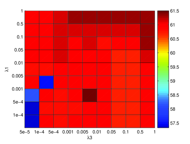
Figure 3: The clustering accuracy of CSC under different parameter settings on the Wiki Text-image dataset.

IV-A4 The parameter setting of CSC

For the proposed CSC method, $\lambda_{1}$ and $\lambda_{3}$ control the prior structure on subspace representations and the pairwise constraints on different modalities respectively. Fig. 3 shows the clustering accuracy as a function of $\lambda_{1}$ and $\lambda_{3}$. The experimental setting is the same as that in the Wiki Text-image dataset. We observe that both of these two parameters are important. More important, there is a large range for $\lambda_{1}$ and $\lambda_{3}$ to make CSC outperform its competitors. The pair-wise constraint corresponding to the regularization $\left\|Z_{A}-Z_{B}\right\|$ plays an important role in CSC. It makes the subspace representations of different modalities close to each other, which potentially leads to an improvement in clustering accuracy. In addition, $\omega_{I}$ balances the importance of each modality. In our experiments, we simply fix them to be the reciprocal of the number of modalities.

Dataset	PCA	LDA	BLM	CCA	LPCCA	PLS	CDFE	SliM2	GMLDA	CMMp
Tr(70)	0.131	0.131	0.134	0.165	0.171	0.176	0.174	0.187	0.199	0.228
Tr(100)	0.132	0.130	0.135	0.174	0.178	0.180	0.182	0.193	0.201	0.233
Tr(130)	0.132	0.130	0.135	0.179	0.181	0.173	0.190	0.194	0.203	0.236

TABLE II: Average MAP scores for text query of different methods over 20 runs. Notations ’Tr(70)’, ’Tr(100)’ and ’Tr(130)’ indicate that 70, 100, and 130 samples per class are randomly selected from the Wiki training dataset for training respectively.

Dataset	PCA	LDA	BLM	CCA	LPCCA	PLS	CDFE	SliM2	GMLDA	CMMp
Tr(70)	9.5$\pm$5.2	10.6$\pm$2.7	12.2$\pm$4.2	33.2$\pm$4.9	35.8$\pm$4.3	25.8$\pm$4.0	34.7$\pm$6.4	36.9$\pm$3.6	21.9$\pm$4.7	41.2$\pm$5.4
Tr(100)	16.2$\pm$5.4	9.9$\pm$5.2	13.5$\pm$7.6	39.4$\pm$5.4	38.7$\pm$4.6	32.5$\pm$5.6	37.1$\pm$3.7	40.8$\pm$4.2	19.6$\pm$4.0	44.0$\pm$5.2
Tr(130)	12.6$\pm$3.1	11.1$\pm$4.7	15.9$\pm$8.0	41.5$\pm$5.5	39.9$\pm$3.5	36.6$\pm$3.5	40.7$\pm$6.5	43.1$\pm$3.3	22.8$\pm$2.5	47.6$\pm$4.8

TABLE III: Average recognition rates and standard deviations for text query by using the KNN (K=10) classifier.

IV-B Cross-modal retrieval

IV-B1 Algorithms

In this subsection, we make use of principal component analysis (PCA), linear discriminant analysis (LDA), canonical correlational analysis (CCA) [2], and partial least squares (PLS) [30][31] as the baselines for cross-modal retrieval. We also compare five cross-modal learning methods, including bilinear model (BLM) for multi-view learning [35], common discriminant feature extraction (CDFE) [7], locality preserving CCA (LPCCA) [33], SliM² [41], and generalized multi-view linear discriminant analysis (GMLDA) [36]. As reported in [36], GMLDA often achieves the highest MAP. Hence we only discuss GMLDA in this section.

Since the number of training samples of each category is different, we randomly select 70, 100 and 130 samples per class from the Wiki training dataset as three training sets respectively. We make use of the Wiki testing dataset as our testing set. Hence the used training and testing sets are different. The parameters of all compared methods are empirically tuned to achieve the best results, and all results are averaged over 20 independent runs. Mean average precision (MAP) and recognition rate are used as the evaluation criterion and $\ell_{2}$ distance is used as the distance function. For MAP, precision at 11 different recall levels {0, 0.1, 0.2, 0.3, 0.4, 0.5, 0.6, 0.7, 0.8, 0.9, 1.0} is used as in [36]; and for recognition rate, we use the $K$ nearest neighbors (KNN) classifier. Since there is ten classes, we set $K$ to 10.

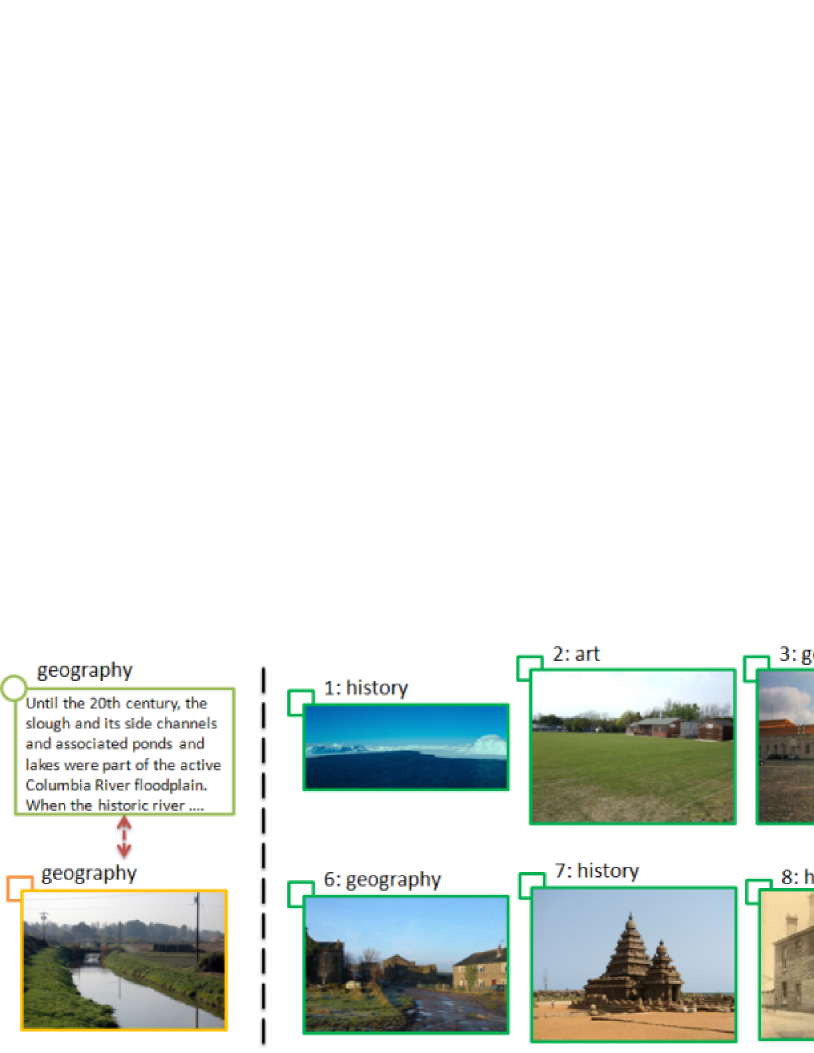
Figure 4: Example of a text query and its corresponding top retrieved images. The left column contains the query text object and its paired image; and the right column lists the top ten retrieved images.

IV-B2 Numerical results on the Wiki dataset

The commonly used Wiki text-image dataset [2][31][36] is used to highlight the benefits of the pairwise constraint. Wiki Text-image dataset consists of 2173/693 (training/ testing) image-text pairs from 10 different semantic classes. It has a 10 dimensional latent Dirichlet allocation model based text features and 128 dimensional SIFT histogram image features.

Table II tabulates average MAP scores for the text query over 20 runs. We see that four baseline methods can be ordered in ascending MAP scores as LDA, PCA, CCA, PLS. Since LDA and PCA do not consider the correlation between different modalities, they fail in cross-modal tasks. It is clear that LPCCA, CDFE, SliM², GMLDA and CMMp perform better than LDA and CCA because they can better use structure information from different modalities. Compared with LPCCA, CDFE, SliM², and GMLDA, our CMMp can handle intra-class variation, pairwise constraint and structure preserving in a framework such that it achieves the highest average MAP scores in all cases.

To further demonstrate the effectiveness of CMMp for cross-modal retrieval, we list recognition rates for text query in Table III. A higher recognition rate indicates that the retrieved top ten images contain more corrected images belonging to the same category of the query text. It is interesting to see that although CDFE and GMLDA have higher MAP scores than CCA, they have lower recognition rates than CCA. This indicates that CDFE and GMLDA obtain a better overall rank than CCA. However, if users only focus on top ten retrieved results, CDFE and GMLDA may perform worse than CCA. Our proposed CMMp achieves the best results in terms of both recognition rates and MAP scores, which also demonstrates the proposed method is potentially powerful for cross-modal learning.

Fig. 4 depicts an example of a text query and its corresponding top retrieved images. We can see that although the category of the text query belongs to ’geography’, its paired image may be more similar to those images in categories ’history’ and ’art’ in the image space. However, five images from ’geography’ are still retrieved by our CMMp method. This may be because our CMMp method can handle both intra-class variation and pairwise constraint.

Dataset	$\ell_{1}$	cosine	ChiSq	SCM[2]	GMA[36]
Tr(70)	0.227	0.265	0.152	0.226	0.232
Tr(100)	0.233	0.271	0.153	0.226	0.232
Tr(130)	0.237	0.278	0.154	0.226	0.232

TABLE IV: Average MAP scores of CMMp for text query under various distance functions over 20 runs.

Dataset	PCA	PCA+LDA	BLM	CCA	LPCCA	PLS	CDFE	SliM2	GMLDA	CMMp
Text query	0.092	0.122	0.115	0.132	0.074	0.144	0.071	0.154	0.170	0.171
Image query	0.058	0.111	0.082	0.103	0.087	0.110	0.084	0.167	0.100	0.170
Average	0.075	0.117	0.099	0.118	0.081	0.127	0.078	0.161	0.135	0.171

TABLE V: MAP scores of different methods on the VOC dataset.

Dataset	LDA	BLM	CCA	LPCCA	PLS	CDFE	GMLDA	CMMp
Text query	0.122	0.172	0.200	0.075	0.181	0.201	0.237	0.245
Image query	0.111	0.118	0.165	0.068	0.156	0.163	0.179	0.213
Average	0.117	0.145	0.183	0.072	0.169	0.182	0.208	0.229

TABLE VI: MAP scores of different methods on the VOC dataset. PCA is used as a preprocessing step for all methods.

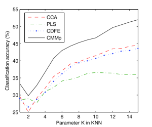
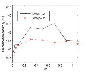
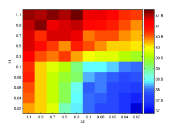
Figure 5: The performance of CMMp under different parameter settings. (a) Classification accuracy as a function of $K$ in KNN classifier. (b) Classification accuracy as a function of $\lambda_{2}$ in CMMp. CMMp-L21 and CMMp-L2 indicate that $\ell_{21}$ norm and $\ell_{2}$ norm are used in the last item in (9) respectively. (c) Classification accuracy as a function of $\lambda_{1}$ and $\lambda_{2}$ in CMMp.

Table IV gives MAP scores under various distance functions. Since semantic correlation matching (SCM) with a linear kernel [2] and generalized multiview analysis (GMA) [36] have shown the state-of-the-art performance for the Wiki text-image dataset, we also report the best results in [2][36]. As in [2], $\ell_{1}$ distance and $\ell_{2}$ distance lead to similar MAP scores. In particular, the cosine distance can significantly improve MAP scores. When we increase the number of training samples in the training, the MAP scores of our proposed method are better than the best results reported in [2][36] if $\ell_{2}$ and $\ell_{1}$ distances are used. Table IV also demonstrates that the MAP scores of our proposed method can be further improved if a suitable distance function is adopted.

IV-B3 Experimental results on the VOC dataset

To further evaluate different cross-modal matching methods, we perform experiments on a subset of Pascal VOC 2007 [70], which consists of collected 5011/4952 (training/testing) image-tag pairs belonging to 20 different categories. We make use of 512-dimensional Gist features and 399-dimensional word frequency features for image and tag respectively. Since there are zero vectors and multi-labeled images, we select the images with only one object from the training and testing set as in [36]. As a result, we obtain 2799 training and 2820 testing data that correspond to 20 classes.

Tables VI and VI show MAP scores of different methods on the VOC dataset without and with PCA as a preprocessing step respectively. We see that when PCA is used as a preprocessing step to remove useless information, MAP scores of almost all cross-modal methods are significantly improved. GMLDA and CMMp perform better than other methods. This may be because they can handle both discriminative and cross-modal information. Since CMMp applies $\ell_{21}$ norms to deal with inaccurate pairs from two modalities, it achieves higher MAP scores than GMLDA.

The imbalance of different modalities and diverse description of image modality make cross modal retrieval more challenging. For example, the first, second and sixth images in Fig. 4 belong to ’history’, ’art’ and ’geography’ categories respectively. However, without any prior knowledge, one may classify all the three images into the ’geography’ category. Compared with image modality, text modality has a narrative (or specific) description [3], which makes text modality be more discriminative. On the VOC dataset (Table VI), the highest MAP scores for text query and image query are 0.245 and 0.213 respectively. An important issue for cross modal retrieval may be to balance the narrow description of text modality and the diverse description of image modality. A potential solution to this issue may be the combination of feature selection to select most relevant image features or regions to narrow the diverse description of image modality.

IV-B4 The parameter setting of CMMp

The regularization parameters in graph embedding based subspace methods often significantly affect the classification accuracy. In this section, we discuss the parameter setting of our proposed cross-modal matching methods.

Classification accuracy as a function of $K$ in KNN classifier is given in Fig. 5 (a). We observe that classification rates of all methods increase quickly as $K$ increases. This may be because more retrieved images corresponding to the input category are selected when $K$ increases. Our CMMp can achieve higher classification rates than the other three methods, which indicates that our method can select more correct images than the other three methods in retrieved top $K$ images. Fig. 5 (a) also gives an explanation that CMMp can obtain better MAP results.

Classification accuracy as a function of $\lambda_{2}$ in CMMp is plotted in Fig. 5 (b). Here we further discuss two regularizers. CMMp-L21 and CMMp-L2 indicate that $\ell_{21}$ norm and $\ell_{2}$ norm are used in the last item in (9) respectively. We observe that CMMp-L21 consistently performs better than CMMp-L2, which indicates the $\ell_{21}$-norm in the last item is necessary. This may be due to outliers in the pairwise constraint of web documents. Image features are often less discriminative than text features such that some text-image pairs are inaccurate.

Classification accuracy as a function of $\lambda_{1}$ and $\lambda_{2}$ in CMMp is shown in Fig. 5 (c). We see that the setting of $\lambda_{1}$ and $\lambda_{2}$ will affect the classification accuracy. The highest classification rate is achieved when both $\lambda_{1}$ and $\lambda_{2}$ are set to be larger than 1. When one of $\lambda_{1}$ and $\lambda_{2}$ is set to a smaller value, classification rates decrease. The variation of classification accuracy indicates that the last two items in (9) play an important role and handle structure preserving and pairwise constraint respectively.

V Conclusion and future work

This paper has systematically studied the pairwise constraint problems in cross-modal learning, and has proposed a general regularization framework for developing cross-modal learning algorithms. For unsupervised learning, a cross-modal subspace clustering method has been proposed to learn a common structure for different modalities; and for supervised learning, a cross-modal matching method has been proposed for multimedia retrieval. Extensive experiments on the Wiki and VOC datasets demonstrate that the joint text and image modeling with pairwise constraint can improve clustering or matching accuracy. In the future, one potential direction is to apply the proposed framework in (1) to discriminative dictionary learning with paired samples [11][12]. Another direction may be to narrow the diverse description of image modality by combining coupled feature selection in (1) to select most relevant image features or regions, or using deep learning to learn more discriminative and related feature representations.

Appendix A The Convergence of Algorithm 2

Proposition 1

Algorithm 2 monotonically decreases the objective function in (9) in each iteration, and converges to the global optimum.

Proof:

According to the properties of the minimization function in half-quadratic optimization [59][58], we have,

$$J(U_{I}^{t-1},p^{I(t)},q^{t})\leq J(U_{I}^{t-1},p^{I(t-1)},q^{t-1}).$$

And according to (12), we obtain,

$$J(U_{I}^{t},p^{I(t)},q^{t})\leq J(U_{I}^{t-1},p^{I(t)},q^{t})\leq J(U_{I}^{t-1},p^{I(t-1)},q^{t-1}).$$

Therefore, Algorithm 2 monotonically decreases the objective function in (9).

In addition, for convex functions $f(x)$ and $g(x)$, $h(x)=f(x)+g(x)$ and $h(x)=f(Dx+b)$ are also convex functions, where $x\in R^{2n}$, $D\in R^{2n\times 2n}$, and $b\in R^{2n}$. Since we can reformulate $\left\|{X_{A}^{T}U_{A}-X_{B}^{T}U_{B}}\right\|_{21}$ as an affine map ($h(x)=f(Dx)$), (9) is joint convex with respect to $U_{A}$ and $U_{B}$. Taking the derivative of (9) w.r.t $U_{A}$ and $U_{B}$, and setting the derivative to zero, we arrive at:

$$U_{A}=X_{A}(I+\lambda_{1}L_{A}+\lambda_{2}Q)X_{A}^{T}\backslash(X_{A}\hat{Y}_{A}),$$ (23)

$$U_{B}=X_{B}(I+\lambda_{1}L_{B}+\lambda_{2}Q)X_{B}^{T}\backslash(X_{B}\hat{Y}_{B}),$$ (24)

where

$$L_{A}=D^{A}-W^{A},W^{A}_{ij}=w_{ij}p_{ij}^{A},D^{A}_{ii}=\sum\nolimits_{j}{W_{ij}^{A}},$$

$$L_{B}=D^{B}-W^{B},W^{B}_{ij}=w_{ij}p_{ij}^{B},D^{B}_{ii}=\sum\nolimits_{j}{W_{ij}^{B}},$$

$$\hat{Y}_{A}=Y+\lambda_{2}QX_{B}U_{B},\hat{Y}_{B}=Y+\lambda_{2}QX_{A}U_{A},$$

$$p^{I}_{ij}=1/{\left\|{U_{I}^{T}(x_{i}^{I}-x_{j}^{I})}\right\|_{2}},$$

$$Q_{ii}=q_{i}=1/{\left\|{U_{A}^{T}x_{i}^{A}-U_{B}^{T}x_{i}^{B})}\right\|_{2}}.$$

Since the problem in (9) is a joint convex problem, $U_{A}$ and $U_{B}$ are a global optimum solution to the problem if and only if (23) and (24) are satisfied.

Since Algorithm 2 will monotonically decrease the objective function in (9) in each iteration $t$, $U_{I}^{t}$, $p^{It}$ and $q^{t}$ will satisfy (23) and (24) in the convergence. As the problem in (9) is a joint convex problem, satisfying (23) and (24) indicates that $U_{I}$ is a global optimum solution to the problem in (9). As a result, Algorithm 2 will converge to the global optimum of (9). ∎

References

- [1] R. Bekkerman and J. Jeon, “Multi-modal clustering for multimedia collections,” in CVPR, 2007.
- [2] N. Rasiwasia, J. C. Pereira, E. Coviello, G. Doyle, G. R. Lanckriet, R. Levy, and N. Vasconcelos, “A new approach to cross-modal multimedia retrieval,” in ACM MM, 2010.
- [3] M. S. Yangqing Jia and T. Darrell, “Learning cross-modality similarity for multinomial data,” in ICCV, 2011, pp. 2407–2414.
- [4] H. Tong, J. He, M. Li, C. Zhang, and W. Ma, “Graph based multi-modality learning,” in ACM MM, 2005.
- [5] M. Kan, S. Shan, H. Zhang, S. Lao, and X. Chen, “Multi-view discriminant analysis,” in ECCV, 2012.
- [6] Y. Luo, D. Tao, C. Xu, C. Xu, H. Liu, and Y. Wen, “Multiview vector-valued manifold regularization for multilabel image classification,” TNNLS, vol. 24, no. 5, pp. 709–722, 2013.
- [7] D. Lin and X. Tang, “Inter-modality face recognition,” in ECCV, 2006, pp. 13–26.
- [8] Z. Cui, W. Li, D. Xu, S. Shan, and X. Chen, “Fusing robust face region descriptors via multiple metric learning for face recognition in thewild,” in CVPR, 2012.
- [9] D. Yogatama and K. Tanaka-Ishii, “Multilingual spectral clustering using document similarity propagation,” in Empirical Methods in Natural Language Processing, 2009.
- [10] S. Sun and J. Shawe-Talyor, “Sparse semi-supervised learning using conjugate functions,” Journal of Machine Learning Research, pp. 2423–2455, 2010.
- [11] H. Guo, Z. Jiang, and L. S. Davis, “Discriminative dictionary learning with pairwise constraints,” in ACCV, 2012.
- [12] K. Jia, X. Wang, and X. Tang, “Image transformation based on learning dictionaries across image spaces,” IEEE TPAMI, vol. 35, no. 2, pp. 367–380, 2013.
- [13] E. Elhamifar and R. Vidal, “Sparse subspace clustering: Algorithm, theory, and applications,” IEEE TPAMI, vol. 35, no. 11, pp. 2765–2781, 2013.
- [14] G. Liu, Z. Lin, and Y. Yu, “Robust subspace segmentation by low-rank representation,” in ICML, 2010.
- [15] G. Liu and S. Yan, “Latent low-rank representation for subspace segmentation and feature extraction,” in ICCV, 2011.
- [16] C.-Y. Lu, H. Min, Z.-Q. Zhao, L. Zhu, D.-S. Huang, and S. Yan, “Robust and efficient subspace segmentation via least squares regression,” in ECCV, 2012.
- [17] S. Basu, A. Banerjee, and R. J. Mooney, “Active semi-supervision for pairwise constrained clustering,” in SDM, 2004.
- [18] H. Cho, I. Dhillon, Y. Guan, and S. Sra, “Minimum sum-squared residue co-clustering of gene expression data,” in ICDM, 2004.
- [19] V. Vindhwani, P. Niyogi, and M. Belkin, “A co-regularization approach to semi-supervised learning with multiple views,” in ICML, 2005.
- [20] A. Kumar and H. Daume, “A co-training approach for multi-view spectral clustering,” in ICML, 2011.
- [21] A. Kumar, P. Rai, and H. Daume, “Coregularized multiview spectral clustering,” in NIPS, 2011.
- [22] Y. Kang, S. Kim, and S. Choi, “Deep learning to hash with multiple representations,” in ICDM, 2012.
- [23] N. Srivastava and R. Salakhutdinov, “Learning representations for multimodal data with deep belief nets,” in ICML, 2012.
- [24] B. Wang, J. Jiang, W. Wang, Z.-H. Zhou, and Z. Tu, “Unsupervised metric fusion by cross diffusion,” in CVPR, 2012.
- [25] Y. Yang, X. Chu, F. Liang, and T. S. Huang, “Pairwise exemplar clustering,” in AAAI, 2012.
- [26] E. Elhamifar, G. Sapiro, and R. Vidal, “Finding exemplars from pairwise dissimilarities via simultaneous sparse recovery,” in NIPS, 2012.
- [27] H. Wang, F. Nie, and H. Huang, “Multi-view clustering and feature learning via structured sparsity,” in ICML, 2013.
- [28] M. Hua and J. Pei, “Clustering in applications with multiple data sources - a mutual subspace clustering approach,” Neurocomputing, vol. 92, pp. 133–144, 2012.
- [29] T.-K. Kim, J. Kittler, and R. Cipolla, “Discriminative learning and recognition of image set classes using canonical correlations,” IEEE TPAMI, vol. 29, no. 6, pp. 1005–1018, 2007.
- [30] A. Sharma and D. W. Jacobs, “Bypassing synthesis: PLS for face recognition with pose, low-resolution and sketch,” in CVPR, 2011, pp. 593–600.
- [31] Y. Chen, L. Wang, W. Wang, and Z. Zhang, “Continuum regression for cross-modal multimedia retrieval,” in ICIP, 2012.
- [32] T. Diethe, D. R. Hardoon, and J. Shawe-Taylor, “Multiview fisher discriminant analysis,” in NIPS Workshop on Learning from Multiple Sources, 2008.
- [33] T. Sun and S. Chen, “Locality preserving CCA with applications to data visualization and pose estimation,” Image and Vision Computing, vol. 25, no. 5, pp. 531–543, 2007.
- [34] N. Quadrianto and C. Lampert, “Learning multi-view neighborhood preserving projections,” in ICML, 2011.
- [35] J. B. Tenenbaum and W. T. Freeman, “Separating style and content with bilinear models,” Neural Computation, vol. 12, pp. 1247–1283, 2000.
- [36] A. Sharma, A. Kumar, H. Daume, and D. W. Jacobs, “Generalized multiview analysis: A discriminative latent space,” in CVPR, 2012.
- [37] S. Yan, D. Xu, B. Zhang, H. Zhang, Q. Yang, and S. Lin, “Graph embedding and extensions: a general framework for dimensionality reduction,” IEEE TPAMI, vol. 29, no. 1, pp. 40–51, 2007.
- [38] J. Weston, S. Bengio, and N. Usunier, “Large scale image annotation: Learning to rank with joint word-image embeddings,” in ECML, 2010.
- [39] A. Lucchi and J. Weston, “Joint image and word sense discrimination for image retrieval,” in ECCV, 2012.
- [40] J. Sang and C. Xu, “Faceted subtopic retrieval: Exploiting the topic hierarchy via a multi-modal framework,” Journal of Multimedia, vol. 7, no. 1, pp. 9–20, 2012.
- [41] Y. Zhuang, Y. Wang, F. Wu, Y. Zhang, and W. Lu, “Supervised coupled dictionary learning with group structures for multi-modal retrieval,” in AAAI, 2013.
- [42] D. Lin and X. Tang, “Coupled space learning of image style transformation,” in ICCV, 2005.
- [43] G. Ye, D. Liu, I.-H. Jhuo, and S.-F. Chang, “Robust late fusion with rank minimization,” in CVPR, 2012.
- [44] B. Kulis, K. Saenko, and T. Darrell, “What you saw is not what you get: Domain adaptation using asymmetric kernel transforms,” in CVPR, 2012, pp. 1785–1792.
- [45] X. Chen, S. Chen, H. Xue, and X. Zhou, “A unified dimensionality reduction framework for semi-paired and semi-supervised multi-view data,” Pattern Recognition, vol. 45, no. 5, pp. 2005–2018, 2012.
- [46] Q. Qian, S. Chen, and X. Zhou, “Multi-view classification with cross-view must-link and cannot-link side information,” Knowledge-Based Systems, vol. 54, pp. 137–146, 2013.
- [47] C. Xu, D. Tao, and C. Xu, “Large-margin multi-view information bottleneck,” IEEE TPAMI, in press, 2014.
- [48] Y. Jiang, J. Liu, Z. Li, and H. Lu, “Semi-supervised unified latent factor learning with multi-view data,” Machine Vision and Applications, in press, 2014.
- [49] J. He and R. Lawrence, “A graph-based framework for multi-task multi-view learning,” in ICML, 2012.
- [50] J. Zhou, J. Chen, and J. Ye, “MALSAR: Multi-task learning via structural regularization,” http://www.public.asu.edu/ jye02 /Software/MALSAR, 2012.
- [51] V. Sindhwani, P. Niyogi, and M. Belkin, “A co-regularization approach to semi-supervised learning with multiple views,” in ICML Workshop on Learning with Multiple Views, 2005.
- [52] U. Brefeld, T. Gartner, T. Sheffer, and S. Wrobel, “Efficient co-regularized least squares regression,” in ICML, 2006, pp. 137–144.
- [53] V. Sindhwani and D. Rosenberg, “An rkhs for multi-view learning and manifold co-regularization,” in ICML, 2008, pp. 976–983.
- [54] S. Petry, C. Flexeder, and G. Tutz, “Pairwise fused lasso,” University of Munich, Tech. Rep., 2011.
- [55] J. Shi and J. Malik, “Normalized cuts and image segmentation,” TPAMI, vol. 22, no. 8, pp. 888–905, 2000.
- [56] D. Cai, X. He, and J. Han, “Spectral regression for efficient regularized subspace learning,” in ICCV, 2007.
- [57] J. Ye, “Least squares linear discriminant analysis,” in ICML, 2007.
- [58] R. He, T. Tan, L. Wang, and W.-S. Zheng, “L21 regularized correntropy for robust feature selection,” in CVPR, 2012.
- [59] F. Nie, H. Huang, X. Cai, and C. Ding, “Efficient and robust feature selection via joint -norms minimization,” in NIPS, 2010, pp. 1813–1821.
- [60] R. He, W.-S. Zheng, B.-G. Hu, and X.-W. Kong, “Two-stage nonnegative sparse representation for large-scale face recognition,” IEEE TNNLS, vol. 24, no. 1, pp. 35–46, 2013.
- [61] C. C. Paige and M. A. Saunders, “Algorithm 583 lsqr: Sparse linear equations and least squares problems,” ACM Transactions on Mathematical Software, vol. 8, no. 2, pp. 195–209, 1982.
- [62] R. He, W.-S. Zheng, and B.-G. Hu, “Maximum correntropy criterion for robust face recognition,” IEEE TPAMI, vol. 33, no. 8, pp. 1561–1576, 2011.
- [63] J. Feng, Z. Lin, H. Xu, and S. Yan, “Robust subspace segmentation with block-diagonal prior,” in CVPR, 2014.
- [64] H. Hu, Z. Lin, J. Feng, and J. Zhou, “Smooth representation clustering,” in CVPR, 2014.
- [65] K. Tang, R. Liu, Z. Su, and J. Zhang, “Structure-constrained low-rank representation,” IEEE TNNLS, 2014.
- [66] Q. Gu and J. Zhou, “Learning the shared subspace for multi-task clustering and transductive transfer classification,” in ICDM, 2009.
- [67] V. R. de Sa, “Spectral clustering with two views,” ICML Workshop on Learning with Multiple Views, 2005.
- [68] J. Liu, C. Wang, J. Gao, and J. Han, “Multi-view clustering via joint nonnegative matrix factorization,” SDM, 2013.
- [69] W.-Y. Chen, Y. Song, H. Bai, C.-J. Lin, and E. Y. Chang, “Parallel spectral clustering in distributed systems,” TPAMI, vol. 33, no. 3, pp. 568–586, 2011.
- [70] S. Hwang and K. Grauman, “Reading between the lines: Object localization using implicit cues from image tags,” IEEE TPAMI, vol. 34, no. 6, pp. 1145–1158, 2011.