Digitization of sunspot drawings by Spörer made in 1861–1894

Abstract

Most of our knowledge about the Sun’s activity cycle arises from sunspot observations over the last centuries since telescopes have been used for astronomy. The German astronomer Gustav Spörer observed almost daily the Sun from 1861 until the beginning of 1894 and assembled a 33-year collection of sunspot data covering a total of 445 solar rotation periods. These sunspot drawings were carefully placed on an equidistant grid of heliographic longitude and latitude for each rotation period, which were then copied to copper plates for a lithographic reproduction of the drawings in astronomical journals. In this article, we describe in detail the process of capturing these data as digital images, correcting for various effects of the aging print materials, and preparing the data for contemporary scientific analysis based on advanced image processing techniques. With the processed data we create a butterfly diagram aggregating sunspot areas, and we present methods to measure the size of sunspots (umbra and penumbra) and to determine tilt angles of active regions. A probability density function of the sunspot area is computed, which conforms to contemporary data after rescaling.

1 Introduction

With the advent of the telescope 400 years ago the longest record of direct evidence of solar activity began. Sunspots are emergences of localized magnetic flux, but their statistics indicate that they are also manifestations of a large-scale magnetic field in the solar interior. There are many statistical properties that can be derived from sunspots such as their spatial distributions across the hemispheres as well as within sunspot groups, their areas and life-times, or their rotation and motion relative to the photosphere. It is desirable to construct time series of sunspot positions and areas of as much of the 400-year period as possible.

Long series of observations in the pre-photographic period are available from, e.g., Johann Caspar Staudacher who observed in 1749–1796 (Arlt 2008, 2009a), James Archibald Hamilton and William Gimingham 1795–1797 (Arlt 2009b), Honoré Flaugergues 1788–1830 (Wolf 1861), Samuel Heinrich Schwabe 1825–1867 (Arlt et al. 2013), Richard Christopher Carrington 1853–1861 (Carrington 1863), and Gustav Spörer 1861–1894 (present work). The references point to detailed analyses, and some of them include positions. Meanwhile the first regular photographic observations started in Greenwich in 1874 (Baumann & Solanki 2005); data of earlier visual observations are also available.

Due to the nature of seeing, the photographs of the Greenwich observations show much less detail than visual data, rendering the early Greenwich data inferior. In the subsequent analysis of Spörer’s sunspot data, only the average positions of groups and total areas were compiled in a database, while additional, useful information can be obtained from individual sunspot positions and areas which are contained in the visual data set. If the visual data is recovered and analyzed, it becomes possible to estimate the area of individual sunspots and to determine the tilt angles of bipolar groups as well as other properties depending on the progress of the solar cycle.

The original visual observations by Spörer are apparently lost, while his printed articles contain detailed synoptic maps of the Sun with the observed sunspot groups. They contain much more information than Spörer’s own measurements.

Spörer’s measurements from 1883–1893, collected in tables, were used to calculate the solar rotation and compare it with the solar rotation derived from observations made in Greenwich and Kanzelhöhe (Balthasar & Fangmeier 1988; Wöhl & Balthasar 1989).

The present study aims at adding one mosaic piece to the 400-year record of sunspot observations by extracting the positional and area information from the visual observations by Gustav Spörer who observed in 1861–1894.

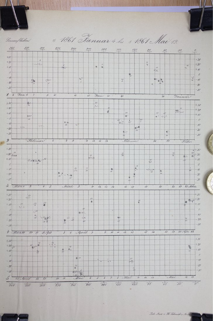
Figure 1: Original drawings with five solar rotation periods after digitization. The title line shows the period of observations. The number of each rotation period and the observing date are marked in the left corner and under each rotation period, respectively. Binder clips and heavy metal coins are used to flatten the paper.

2 Observations

Born in 1822 in Berlin, Friedrich Wilhelm Gustav Spörer studied mathematics and astronomy at the University of Berlin. In 1843 Spörer obtained his degree and started to work on his dissertation at the Observatory in Berlin. After becoming an instructor in Anklam in 1849 his interest in sunspots peaked and led to the start of his observations on 2 December 1860 (Spörer 1861). He published his results in numerous articles in Publicationen des Astrophysikalischen Observatoriums zu Potsdam and Publicationen der Astronomischen Gesellschaft (Spörer 1874, 1878, 1880, 1886, 1894). Later, in 1874, he moved to Potsdam and worked at the Astrophysical Observatory, where he continued his observations of sunspots until 1894. Spörer died in 1895 in Gießen while traveling (Vogel 1895).

Spörer is famous for his simplification of Richard Carrington’s theory about sunspot latitudes in a solar cycle which is known as Spörer’s Law. It was also Spörer who found a minimum of solar activity between about 1645 and 1715 with the few spots appearing between 1672 and 1704 all being on the southern hemisphere (Spörer 1887). This minimum (1645–1715) was named after the English astronomer Edward Walter Maunder. But an earlier minimum from 1420–1570, found with the ¹⁴C method (Usoskin et al. 2007; Bard et al. 1997), is now termed Spörer minimum in honor of Spörer’s discovery of the Maunder minimum (Eddy 1976).

Long continuous observations of sunspots were made by Samuel Heinrich Schwabe 1825–1867 (Arlt 2011). In this time period, Carrington started his observations in 1853, which were continued by Spörer’s observations beginning in January 1861 during Carrington rotation period No. 96. Carrington arranged the sunspots of one solar rotation period according to their heliographic longitudes and latitudes. Spörer used the same method allowing to connect both data sets. There are two ways in which Spörer provides us with data on sunspots:

• Sunspot synoptic maps similar to Carrington’s synoptic charts but differ by an offset in longitude.

• Tables with measurements of sunspot positions on various days of the visibility period of a group. In this way, the disk passage of the sunspot groups can be visualized.

Spörer used different telescopes for his observations. First he used a 3$\nicefrac{{1}}{{2}}$-foot telescope and after 1865 a 7-foot telescope (Spörer 1874). Units commonly used in Prussia at that time are given in Noback & Noback (1851). In 1868, he received a new telescope, with a 5-inch Steinheil lens, as a present from the crown prince of Prussia for his research (Vogel 1895; Spörer 1874). Since 1879 he observed with a 7$\nicefrac{{1}}{{2}}$-inch diameter Grubb refractor (Spörer 1878, 1880, 1886, 1894) at the Astrophysical Observatory Potsdam. After 1884 photographic plates were used for the observations. But Spörer still observed sunspots visually with the telescope. In general, it was easier to find sunspots first with the telescope before capturing them on photographic plates. The telescope was also helpful when the sky was cloudy. During short breaks in the clouds it was possible to quickly gauge sunspot positions and shapes visually, while it was hopeless to take a photograph. In bad seeing conditions bigger sunspots were still faintly visible on the photographic plates but small spots were indeterminable (Spörer 1894).

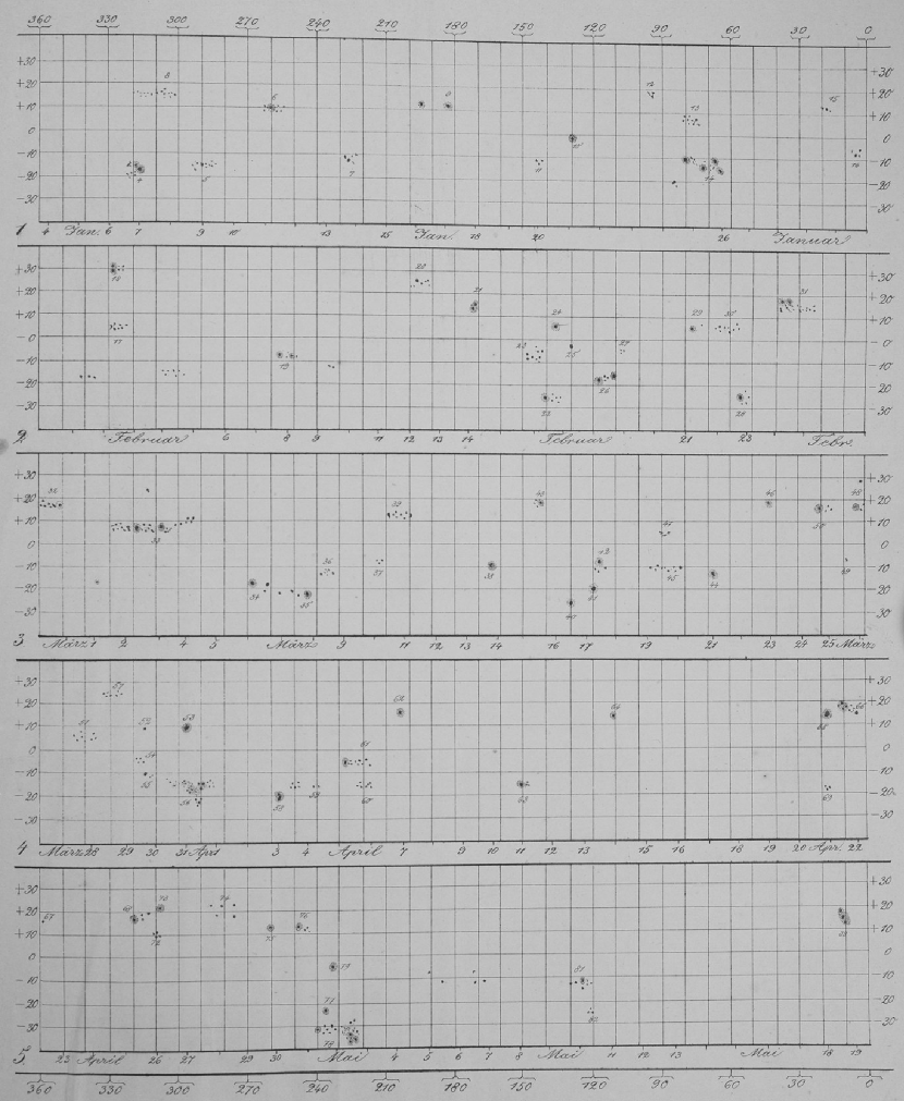
Figure 2: Rotated and cropped image (left) after correction by a background image (“pseudo flat-field”) derived from an order-statistics filter (right). Both images are displayed on a linear scale between the minimum and maximum of their respective intensities.

If observations were out of question because of bad weather or other circumstances, Spörer used the data from other observatories in Vienna, Münster, or Rome to augment his data set (Spörer 1874). Auxiliary entries are marked with characters in the data tables. Especially in the beginning he received data from Prof. Eduard Heis in Münster, which he labeled with an $H$. Spörer carried out most of his observations at local noon. He noted date and time of his sunspot observations, and he measured the position angle $p$ relative to the terrestrial equator and the geocentric angular distance $\rho$ from the middle of the solar disk. With these two variables it is possible to calculate the heliographic coordinates, i.e., the longitude $l$ and the latitude $b$. Once longitude and latitude are known, the normalized longitude $L$ as shown in Fig. 1 can be computed (for details see Spörer 1874). The coordinates $b$ and $L$ of the day of meridian passage were used to draw the sunspots. The abscissa shows the normalized longitude $L$ from 360^∘ to 0^∘ while the ordinate is the heliographic latitude $b$ in the range of $\pm 40^{\circ}$ for one rotation period. Each of the 89 pages contains five rotation periods (Fig. 1) amounting to 445 rotation periods in total. The sunspot drawings were published as lithographs, which even show details of sunspots such as umbra and penumbra (Fig. 7).

3 Image processing

3.1 Image capture and digitization

The sunspot drawings were collated in hardbound books with rigid covers, where several signatures (folded sheets of paper) are stitched together in the books’ spines. Consequently, pages will not be perfectly flat when opening the books. Binder clips and heavy metal coins are used to flatten the drawings (Fig. 1) in preparation for acquiring digital images. All images are taken by artificial light from two bright desk lamps under the same conditions.

Whole pages are photographed with a Canon EOS 5D digital camera, which records images with $4368\times 2912$ pixels. The Sigma 50 mm $f/2.8$ EX DG macro lens ensures that image distortions are minimal over the field-of-view, while small perspective errors may remain and are easily corrected later. The image scale of the recorded images is about 0.35 mm pixel^-1. The 36-bit digital images are preprocessed with the computer program RawTherapee Version 2.4.1 and saved as 24-bit RGB images in the Tagged Image File Format (TIFF). The filenames (spoererYYYYMMDD$\_$YYYYMMDD.tif) are created using the start and end dates of the first and last rotation periods depicted in the images, respectively.

3.2 Removal of artifacts and conditioning of images

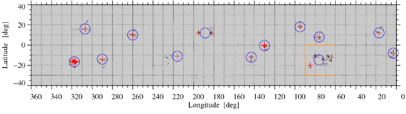
Figure 3: Image after remapping with identified regions from Spörer’s measurements. The red crosses refer to the positions of the sunspots and the blue circles mark the mean positions of the sunspot groups. The positions were measured over several days, i.e., it is possible to visualize the transit of the sunspot group across the solar disk. Sometimes there are errors in the data (see Sect. 3.4), e.g., the table entry of spot group No. 7 differs from its position in the longitude-latitude map. Properties of spot group No. 14 (orange square) are discussed in Sect. 3.7.

The sunspot drawings were published nearly 150 years ago, thus, the pages are yellowish, stained, and corrugated. These artifacts have to be removed because they will severely affect the analysis of sunspot properties. All algorithms hereafter are developed in the Interactive Data Language (IDL). For the most part, the programs run with a minimum of user interaction to avoid potential biases.

Initially, the three-component color images are converted to gray-scale images by simply averaging their color planes. The images are rotated by $90\mbox{${}^{\circ}$}$ to have them in portrait format as in the books. The bitmaps are then cropped so that only the coordinate grids with sunspot data and their annotations remain. In the next processing step, a small position angle error of the camera has to be measured and removed. The grid lines are the dominant feature in the images, thus, averaging all rows and all columns results in two intensity traces with sharp minima at the $x$- and $y$-coordinates of the grid lines, respectively. The standard deviation of the intensity traces will reach a maximum, when the angular offset is zero. Therefore, we rotate the images in steps of $0.1\mbox{${}^{\circ}$}$ within the range of $\pm 1\mbox{${}^{\circ}$}$ and compute the respective standard deviations. A parabolic fit to this curve yields the exact angle by which the images have to be rotated. Cubic spline interpolation (Park & Schowengerdt 1983) is used to minimize interpolation errors between pixels. An order-statistics filter is used to compute a background intensity map, thus, eliminating the grid lines, annotations, and sunspots (Fig. 2). The most common order-statistics filter are minimum, maximum, and median filters (e.g., Gonzalez & Woods 2002). However, none of them provides an acceptable map of background intensities. Therefore, we implemented a filter, which ranks the intensities within a 33$\times$33-pixel neighborhood and replaces the value of the center pixel with the value that represents the $80^{\mathrm{th}}$ percentile of the intensity distribution. The 16-pixel wide borders of the full background intensity map are simply replaced by the mean background intensity.

The effect of such a non-linear spatial filter is to replace clusters or lines of dark pixels by gray levels, which resemble more closely their neighborhood. Closer inspection of the right panel in Fig. 2 reveals that the procedure captures well the global intensity trends, which are evident in the lower-left and upper-right corners. In addition, faint shadows created by the wrinkled paper are efficiently removed. What appears at a first glance as a potentially bothersome artifact, i.e., a faint brightening associated with grid lines and annotations, augments the contrast in the next image processing step. Division of an image by its background intensity map, which correspond to a pseudo flat-fielding procedure, results in an artificially “bleached” and flattened image (left panel in Fig. 2). This corrected image still contains distortions due to wrinkling of the paper and because of the curvature of pages photographed from an opened hardbound book.

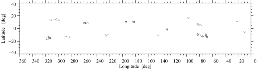
Figure 4: Image after applying morphological image processing to remove the grid lines. The sunspots are now clearly visible. In addition, the sunspot group numbers have been removed with a point-and-click procedure.

3.3 Geometric correction and resampling of images

The first step in geometrically correcting distorted images is to extract the exact pixel coordinates, where the horizontal and vertical grid lines intersect. We construct a 17$\times$17-pixel kernel by setting the values of two intersecting, three-pixel wide horizontal and vertical lines to unity and keeping all other pixels at zero. Convolving the corrected image with such a kernel enhances the grid lines, in particular, where the lines cross each other. Simple thresholding then yields a binary mask in which pixels belonging to the grid have values of unity. Initial estimates of the grid coordinates can be computed from the average profiles of rows and columns, which are smoothed by a 17-pixel wide filter (Lee 1986) and subsequently normalized. Parabolic fits to the local maxima of the row and column profiles are in most cases good estimates of the $x$- and $y$-grid coordinates. Note that the first 51 images contain an extra axis at the bottom of the page displaying the heliographic longitude $L$ in increments of 30^∘. Usually, it is more difficult to determine the $y$-coordinates because of the preferential warping of the pages. Therefore, the average column profiles are computed locally, i.e., only for regions between adjacent vertical grid lines.

In order to determine the maximum in $x$- and $y$-direction, we take the grid line between two grid points and determine the maximum of intensity of this region. Direct-neighbor coordinates are used for points on the border.

Some of the grid coordinates are slightly misplaced. This type of error occurs especially near sunspots. To remedy this, the mean distance to direct neighbors of a grid point is estimated, i.e., the difference between mean distance and actual distance to neighbors can be calculated. This difference should be less than six pixels, otherwise the distance of the neighbors will be replaced by the mean distance. In rare cases (only 10 occurrences) the grid coordinates are off by 30 pixels. In these special cases, the coordinates are replaced by the mean coordinates of columns or rows in this rotation period.

In order to improve the preliminary $x$- and $y$-coordinates, we extract an 8$\times$8-pixel square region from a binary mask, enlarge this region by a factor of 20 using cubic spline interpolation and determine the intensity maximum of this region.

During the second to last step, we take a 140$\times$140-pixel region and double its size. Then the grid is extracted by using a mask to minimize the influence of a sunspot by estimating the maximum intensity of the grid line. The highest intensity appears where two grid lines intersect. The intensity map is smoothed twice using a 141$\times$141-pixel boxcar average to eliminate some spurious features obfuscating the maximum. The maximum in $x$- and $y$-direction is then the new grid coordinate.

Finally, we visually examined all grid coordinates and replace manually the remaining ones that do not match. For this purpose, the region is enlarged in a separate window, and a better coordinate can be chosen by a point-and-click operation with the computer mouse. On average we replaced 1.4 grid points for each rotation period (37$\times$9 grid points).

The heliographic longitudes and latitudes are given in increments of $10\mbox{${}^{\circ}$}$, so that we have a grid of (37$\times$9) $x$- and $y$-coordinates for each rotation period, which is sufficient to resample the distorted grid to a new, equidistantly sampled grid with a resolution of 0.1^∘ pixel^-1. We also include a 5^∘-wide border to minimize sampling errors at the periphery. Subsequently, Delaunay triangulations (Lee & Schachter 1980) are used to interpolate the sunspot data to the new grid (Fig. 3). Data of this type ($3600\times 800$ pixels) are obtained for each of the 445 rotation periods recorded by Spörer and build the input for any further processing.

3.4 Error sources

An electronic version of Spörer’s tabulated measurements was provided by Ilkka Tuominen, Helsinki, which contains the sunspot positions from 1861 to 1884. Note that this period is shorter than the time interval covered by the synoptic maps. Using this table, we compare the sunspot positions in the drawings and the coordinates in the tables (see Fig. 3). In most cases, the coordinates are identical, except for a few cases, e.g., spot No. 7 in Fig. 3, where the positions differ. Table 1 provides the differences in latitude or longitude within the first 100 rotation periods. Most of the erroneous coordinates deviate by exactly 10^∘, but there are also sign errors. We found 18 mismatches within 100 rotation periods with 984 sunspots.

Table 1: Differences in sunspot positions between Spörer’s measurements and coordinates in the first 100 synoptic maps.

Period	Sunspot	Longitude $L$	Coordinates	Coordinates
	number	or latitude $b$	in the table	in the image
01	007	$L$	$-$216∘	$-$226∘
03	046	$L$	$-$031∘	$-$041∘
09	128	$L$	$-$228∘	$-$238∘
09	130	$L$	$-$171∘	$-$181∘
16	021	$L$	$-$109∘	$-$119∘
33	069	$b$	$-$027∘	$-$017∘
33	076	$b$	0$-18^{\circ}$	$-$018∘
35	093	$L$	$-$304∘	$-$314∘
39	132	$L$	$-$128∘	$-$138∘
50	113	$b$	$-$012∘	$-$022∘
53	140	$L$	$-$254∘	$-$264∘
55	005	$b$	0$-11^{\circ}$	0$-15^{\circ}$
62	089	$b$	$-$009∘	$-$019∘
63	103	$L$	$-$053∘	$-$043∘
68	138	$L$	$-$307∘	$-$302∘
69	014	$L$	$-$218∘	$-$207∘
79	067	$L$	$-$043∘	$-$102∘
93	041	$b$	$-$008∘	$-$018∘

• Most positions have differences of exactly 10^∘. We expect them to be mistakes in the lithographic prints.

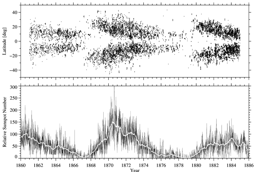
Figure 5: The butterfly diagram (top) contains the positions of all sunspots from 1861 to 1884 listed in the electronic version of Spörer’s tabulated measurements. The SIDC daily relative sunspot numbers from 1860 to 1885 (bottom) are depicted for the daily values (black) and a 200-day, sliding average (white).

3.5 Eliminating grid lines and identifying sunspots

The 3600$\times$800-pixel images contain grid lines, sunspots, and to some extent artifacts, i.e., dust particles, stains, or elongated fissures because of buckling pages. The goal is to identify the sunspots by removing artifacts and grid lines. First, the grayscale images are slightly smoothed and thresholded to yield binary masks. Small-scale artifacts with less than 16 contiguous pixels are eliminated using standard tools for “blob analysis” (Fanning 2011).

Second, removing grid lines is more complicated because they can overlap with sunspots. We start by removing the horizontal grid lines. The grid lines vary in width, but in general, they are not wider than seven pixels. Thus, we create a template, where the horizontal, seven-pixel-wide grid lines correspond to unity and the spaces in between to zero. We now exploit the fact that a sunspot superimposed on a grid line will broaden the line locally. We create a 21$\times$21-pixel kernel, where the pixels of the vertical row through the center are set to $\nicefrac{{1}}{{21}}$ and all other pixels to zero, so that the sum of all values is unity. The width of the kernel is chosen as three times the width of the grid lines. Convolving the binary mask with this kernel and thresholding the result leaves only areas where grid line intersect with sunspots. Simple logic operations are then used to eliminate the horizontal grid lines, and the procedure is repeated for the vertical grid lines. The algorithm sometimes leaves small artifacts of a few contiguous pixels, which are again removed with blob analysis tools.

The resulting binary mask contains only the sunspots, the numbers labeling the sunspot groups, and very few remaining artifacts. Until now, the whole procedure did not require any user interaction. In the final step, group labels and artifacts are removed by a point-and click routine. The result in Fig. 4 shows the grayscale image multiplied by the binary mask, where ultimately only pores, sunspots, and active regions persist. Based on these results we create a butterfly diagram (Sect. 3.6), and we discuss exemplarily how to calculate the tilt angles of the sunspot groups and to determine other sunspot properties (Sect. 3.7). The log-normal probability density function (PDF) of the measured sunspots is compared in Sect. 3.8 with other frequency distributions taken from literature.

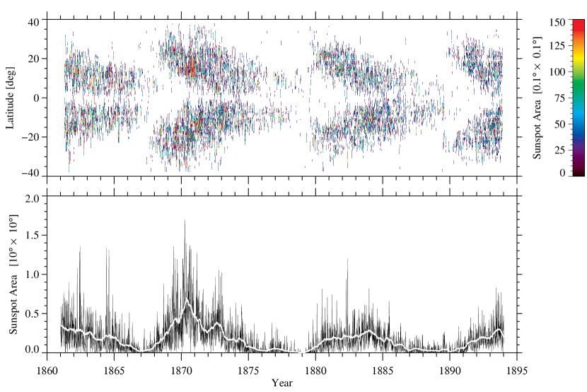
Figure 6: Butterfly diagram (top) with color-coded sunspot areas. The colors indicate the number of occurrence of sunspot pixels with a size of 0.1${}^{\circ}\times$ 0.1^∘ within a 60^∘-wide and 0.4^∘-high longitude-latitude bin. The sunspot area (bottom) is based on the number of pixels with a size of 0.1${}^{\circ}\times 0.1^{\circ}$ in a 60^∘-wide longitude bin (black). The white curve corresponds to a 200-day, sliding average to facilitate comparison with the lower panel of Fig. 5. The units on the ordinate combine 10 000 individual sunspot pixels.

3.6 Butterfly diagram and relative sunspot number

We create a butterfly diagram (top panel of Fig. 5) from the sunspot positions of Spörer’s measurements covering the period from 1861 to 1884. This diagram shows the latitudinal position of the sunspots in the northern and southern hemispheres over a period of 24 years. In the beginning of solar cycle No. 11 (1867–1878), new-cycle sunspots appear at high latitudes, while old-cycle sunspots are still present at low latitudes, in particular in the northern hemisphere. As the cycle progresses, more sunspot groups can be observed at successively lower latitudes. In general, the distribution of sunspots across latitude is more uniform in the southern hemisphere. The sunspots’ migration towards the solar equator over the solar cycle, where the number of spots decreases, is today known as Spörer’s law.

The butterfly diagram is complemented by the daily relative sunspot numbers (bottom panel of Fig. 5), which are obtained from the Solar Influences Data analysis Center (SIDC), Royal Observatory of Belgium (Vanlommel et al. 2004; Clette et al. 2007). The variation of the spot coverage with time is much easier to visualize in a graph. In particular, solar cycle No. 11 shows a pronounced double-peaked maximum (Feminella & Storini 1997) both in the daily sunspot numbers and their 200-day average. Generally, the temporal evolution of solar activity is well correlated in these two data sets.

The processed digital synoptic maps (Sect. 3.5) offer another way to create a butterfly diagram based on the whole time series of the years 1861 to 1894. In principle, one could concatenate all synoptic maps yielding a map with $(445\times 3600)\times 800=1\,602\,000\times 800$ pixel (a 1.3 gigapixel image!), which we transform into a super-synoptic map with $2670\times 200$ pixels, i.e., each pixel contains the number of sunspots pixels in a 60^∘-wide and 0.4^∘-wide longitude-latitude bin. The size of a pixel is $0.1^{\circ}\times 0.1^{\circ}$, thus, the frequency of occurrence of sunspot pixels corresponds to the sunspot area. The result of this compilation is shown in Fig. 6. Visually the butterfly diagrams of Figs. 5 and 6 agree well. However, tight cluster of high sunspot counts are easier seen in Fig. 6, especially, in 1870 in the northern hemisphere. Projecting the two-dimensional frequency distribution onto the time axis produces a graph similar to the daily relative sunspot numbers in the bottom panel of Fig. 5. Note, however, that a 60^∘-wide longitude bin matches about 4.5 days of a solar rotation period. This relationship is also used to compute a 200-day, sliding average, which again is closely correlated to the 200-day average of the SIDC daily relative sunspot numbers.

3.7 Sunspot properties and active region tilt angles

Table 2: Sunspot properties corresponding to Fig. 7.

Sunspot	Perimeter area		Center coordinates			Ellipse fitting
ID	$[1^{\circ}\times 1^{\circ}]$		$L$	$b$		$a$	$\varepsilon$	$\theta$
$\phantom{0}1$	$8.05$		$65.3\mbox{${}^{\circ}$}$	$-15.2\mbox{${}^{\circ}$}$		$2.08\mbox{${}^{\circ}$}$	$0.78$	$-39.8\mbox{${}^{\circ}$}$
$\phantom{0}2$	$7.88$		$72.7\mbox{${}^{\circ}$}$	$-14.0\mbox{${}^{\circ}$}$		$1.73\mbox{${}^{\circ}$}$	$0.44$	$-36.0\mbox{${}^{\circ}$}$
$\phantom{0}3$	$0.30$		$69.4\mbox{${}^{\circ}$}$	$-14.9\mbox{${}^{\circ}$}$		$0.36\mbox{${}^{\circ}$}$	$0.52$	$-$$70.3\mbox{${}^{\circ}$}$
$\phantom{0}4$	$8.56$		$67.5\mbox{${}^{\circ}$}$	$-11.5\mbox{${}^{\circ}$}$		$2.34\mbox{${}^{\circ}$}$	$0.74$	$-80.7\mbox{${}^{\circ}$}$
$\phantom{0}5$	$0.28$		$69.3\mbox{${}^{\circ}$}$	$-12.9\mbox{${}^{\circ}$}$		$0.36\mbox{${}^{\circ}$}$	$0.61$	$-$$77.9\mbox{${}^{\circ}$}$
$\phantom{0}6$	$0.22$		$75.7\mbox{${}^{\circ}$}$	$-12.6\mbox{${}^{\circ}$}$		$0.35\mbox{${}^{\circ}$}$	$0.72$	$-51.4\mbox{${}^{\circ}$}$
$\phantom{0}7$	$1.23$		$76.7\mbox{${}^{\circ}$}$	$-11.2\mbox{${}^{\circ}$}$		$1.17\mbox{${}^{\circ}$}$	$0.90$	$-$$79.4\mbox{${}^{\circ}$}$
$\phantom{0}8$	$7.70$		$80.1\mbox{${}^{\circ}$}$	$-10.8\mbox{${}^{\circ}$}$		$1.86\mbox{${}^{\circ}$}$	$0.62$	$-23.8\mbox{${}^{\circ}$}$
$\phantom{0}9$	$0.45$		$72.1\mbox{${}^{\circ}$}$	$-11.3\mbox{${}^{\circ}$}$		$0.41\mbox{${}^{\circ}$}$	$0.28$	$-34.9\mbox{${}^{\circ}$}$
$10$	$0.82$		$77.9\mbox{${}^{\circ}$}$	0$-9.7\mbox{${}^{\circ}$}$		$0.82\mbox{${}^{\circ}$}$	$0.90$	$-59.2\mbox{${}^{\circ}$}$

Binary masks like the one used to create Fig. 4 are the starting point for determining sunspot properties. Application of blob analysis tools (Fanning 2011) returns parameters such as the sunspot area and the perimeter in pixels, the coordinates of the sunspot’s center-of-gravity (CoG), and from ellipse fitting the semi-major axes $a$, the numerical eccentricity $\varepsilon$, and the orientation $\theta$ of an ellipse encompassing the sunspot. The results are visualized for sunspot group No. 14 in Fig. 7, and the quantitative results are presented in Tab. 2. Still some problems remain. Not all sunspots are recognized as single spots. Nearby spots are often identified as one single spot. As a consequence, the Wolf number will be smaller than expected. In the example, the correct Wolf number is 24, but the Wolf number based on our algorithm is only 20.

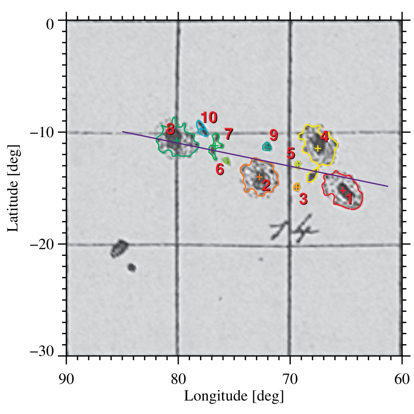
Figure 7: Sunspot group No. 14 with ten identified sunspots. Their properties are given in Tab. 2. A linear fit (blue line) to all pixels belonging to the sunspot group indicates the region’s tilt angle.

Furthermore, we measure the tilt angle of the group, which is $11.6\mbox{${}^{\circ}$}$, by fitting a line to all pixels belonging to the spot group. Joy’s law (McClintock & Norton 2013) indicates that a sunspot group will establish a tilt angle with the leading spot closest to the equator. In this example, the leading spot has the largest distance to the equator. However, the spot group is complex and contains four mature sunspots. Without any additional information about the group’s magnetic configuration or temporal evolution, it is impossible to decide, if the group emerged as one or represents the superposition of two bipolar regions.

Visual inspection of the synoptic maps gives the impression that regular sunspots with well established penumbrae are drawn too large. This might also apply to pores, where pencil marks might already be too coarse to correctly indicate the actual size. The positions, however, of spots are accurately represented in the synoptic maps, with the exception of the errors already noted in Sect. 3.4.

3.8 Probability density function of sunspot areas

Size and location of individual sunspots were already used in creating the butterfly diagram in Fig. 6. Morphological image processing additionally provides access to another important characteristics of sunspots, i.e., the PDF of their areas over the course of 33 years of observations by Spörer.

A pixel with a size of 0.1^∘$\times$0.1^∘ corresponds at the intersection of equator and central meridian to an area of about 1.5 Mm² or 0.5 $\mu$HS (one millionth of the visible solar surface). Lacking a clear description of how the sunspot drawings were transferred to an equidistant longitude-latitude grid, it remains unclear, if geometrical projection effects were taken properly into account. However, projection effects can only introduce an error of about 25%. The annual variations related to Earth’s orbit around the Sun and the solar $B_{0}$-angle (heliographic latitude of the central point of the solar disk) is only about 0.6%, which is negligible compared with other systematic errors. For example, thresholding and morphological dilation/erosion operations can lead to erroneous sunspot boundaries, thus, overestimating sunspot areas by at most a few tens of percent. Even taken together, these effects cannot explain the apparently oversized sunspots in the synoptic maps. Therefore, we decided to compare our PDF of sunspot areas with previous studies.

Figure 8: Probability density functions of areas and radii for sunspots and pores (symbols) and their comparison to previous studies (curves).

Log-normal PDFs of pores and umbral areas are described in Bogdan et al. (1988) and Kiess et al. (2014) for Mount Wilson data (1917–1982) and contemporary observations from space (Solar Dynamics Observatory (SDO, Pesnell et al. 2012), May 2010 to October 2012), respectively. Their PDFs are presented in Fig. 8 as continuous curves, where we used the notation and normalization scheme of the PDF given by Kiess et al. (2014)

$$\ln\left(\frac{dN}{dA}\right)=-\frac{(\ln A-\ln\langle A\rangle)^{2}}{2\ln\sigma_{A}}+\ln\left(\frac{dN}{dA}\right)_{\text{max}},$$ (1)

where $A$ is the umbral/pore size, $(dN/dA)$ is the density function, $\langle A\rangle$ is the mean, and $\sigma_{A}$ is the width of the distribution. A distinguishing characteristics of these PDFs is the spacial resolution, i.e., the minimum spot size of $2$ and $0.5~{}\mu$HS, respectively. Using high resolution G-Band images of the Japanese Hinode mission, Verma & Denker (2014) derived the statistical properties of pores for the time period of October 2006 to August 2013 (open diamonds in Fig. 8). Here, the minimum spot size is just $0.25~{}\mu$HS, which is a good lower threshold for magnetic field concentrations still capable of inhabiting the convective energy transport.

Matching Spörer’s sunspot data to the aforementioned PDFs requires an appropriate scaling of the sunspot areas. The PDF based on Spörer’s data is double-peaked because the morphological image processing algorithm detects both pores (filled pencil marks) and sunspots (filled umbrae and dotted penumbrae surrounded by a thin boundary). The first peak corresponds to the pores and the second peak to the sunspots. We use the minimum between the two peaks as a threshold, which yields an average spot area of 38.9 $\mu$HS for spots with an area smaller than $100~{}\mu$HS. The average size of pores and umbrae in Kiess et al. (2014) is 10.7 $\mu$HS. Therefore, we conclude that the ratio of 13.3 is a conservative estimate of the area scaling factor between SDO and Spörer data.

Using this scaling parameter, we place the Spörer data (solid circles) in the log-log frequency distribution shown in Fig. 8. With this correction, the frequencies of occurrence between 2 and 10 $\mu$HS are very similar to the aforementioned studies. Above 10 $\mu$HS only sunspots with umbrae and penumbrae are counted, thus, the curve is shifted parallel to the right. The strong deviation to lower frequency of the Spörer PDF below $2~{}\mu$HS can be attributed to the limited spacial resolution offered by Spörer’s telescopes. Under ideal conditions the diffraction-limited resolution is about 1000 km on the solar surface. Therefore, a large fraction of small sunspots and pores will be missed in Spörer’s observations. Despite the limitations imposed by the scaling factor, we are in this manner able to present a self-consistent approach to place Spörers historic sunspot data into the parameter space of studies from the $20^{\mathrm{th}}$ and $21^{\mathrm{st}}$ century.

4 Summary

There are several ways of extracting information about position and size from historical sunspot drawings. A fully manual method was employed by Arlt (2009a) and Arlt et al. (2013) on the drawings by Staudacher and Schwabe, respectively. A semi-automatic procedure was used by Cristo et al. (2011), who analyzed the sunspot observations by Ludovic Zucconi in 1754–1760. They picked spots manually and determined their area automatically. In the present work, we put forward a procedure for automatic extraction of positions and sizes of sunspots in historical records and applied it to observations from 1861–1894 by Gustav Spörer. It was possible to process the images of his synoptic maps and to obtain good results – despite some difficulties related to the scale of the sunspot in the drawings. Ultimately, a 150-year-old data set of sunspot observations is now available for contemporary data analysis facilitating the study of the Sun’s activity in the past. The data presented in this article are available upon request by contacting one of the authors.