Combining regional estimation and historical floods: a multivariate semi-parametric peaks-over-threshold model with censored data

Abstract.

The estimation of extreme flood quantiles is challenging due to the relative scarcity of extreme data compared to typical target return periods. Several approaches have been developed over the years to face this challenge, including regional estimation and the use of historical flood data. This paper investigates the combination of both approaches using a multivariate peaks-over-threshold model, that allows estimating altogether the intersite dependence structure and the marginal distributions at each site. The joint distribution of extremes at several sites is constructed using a semi-parametric Dirichlet Mixture model. The existence of partially missing and censored observations (historical data) is accounted for within a data augmentation scheme. This model is applied to a case study involving four catchments in Southern France, for which historical data are available since 1604. The comparison of marginal estimates from four versions of the model (with or without regionalizing the shape parameter; using or ignoring historical floods) highlights significant differences in terms of return level estimates. Moreover, the availability of historical data on several nearby catchments allows investigating the asymptotic dependence properties of extreme floods. Catchments display a a significant amount of asymptotic dependence, calling for adapted multivariate statistical models.

¹ Institut Mines-Télécom, Télécom ParisTech, CNRS LTCI
37-38, rue Dareau, 75014 Paris, FRANCE
anne.sabourin@telecom-paristech.fr

² Institut National de Recherche en Sciences et Technologies pour l’Environnement et l’Agriculture, Centre de Lyon
5 rue de la Doua - CS70077, 69626 VILLEURBANNE Cedex, France

Keywords:  Multivariate extremes; censored data; semi-parametric Bayesian inference; mixture models; reversible-jump algorithm

1. Introduction

Statistical analysis of extremes of uni-variate hydrological time series is a relatively well chartered problem. Two main representations can be used in the context of extreme value theory (e.g. Madsen et al., 1997b, ; Coles,, 2001): block maxima (typically, annual maxima) can be modeled using a Generalized Extreme Value (GEV) distribution (see e.g. Hosking,, 1985), while flood peaks over a high threshold (POT) are commonly modeled with a Generalized Pareto (GP) distribution (see e.g. Hosking and Wallis,, 1987; Davison and Smith,, 1990; Lang et al.,, 1999). One major issue in at-site flood frequency analysis is related to data scarcity (Neppel et al.,, 2010): as an illustration, most of the recorded flood time series in France are less than $50$ years long, whereas flood return periods of interest are typically well above $100$ years. Moreover, an additional challenge arises if one is interested in multivariate extremes at several locations. A complete understanding of the joint behavior of extremes at different locations requires to model their dependence structure as well. While there exists a multivariate extreme value theory (e.g. Coles and Tawn,, 1991; De Haan and De Ronde,, 1998), its practical application is much more challenging than with standard univariate approaches.

1.1. Regional estimation

In order to address the issue of data scarcity in at-site flood frequency analysis, hydrologists have developed methods to jointly use data from several sites: this is known as Regional Frequency Analysis (RFA) (e.g. Hosking and Wallis,, 1997; Madsen and Rosbjerg,, 1997; Madsen et al., 1997a, ). The basis of RFA is to assume that some parameters governing the distributions of extremes remain constant at the regional scale (see e.g. the ’Index Flood’ approach of Dalrymple,, 1960). All extreme values recorded at neighboring stations can hence be used to estimate the regional parameters, which increases the number of available data.

The joint use of data from several sites induces a technical difficulty: the spatial dependence between sites has to be modeled. A common assumption has been to simply ignore spatial dependence by assuming that the observations recorded simultaneously at different sites are independent, which is often unrealistic (see Stedinger,, 1983; Hosking and Wallis,, 1988; Madsen and Rosbjerg,, 1997, for appraisals of this assumption). An alternative approach uses elliptical copulas to describe spatial dependence (Renard and Lang,, 2007; Renard,, 2011). While this approach allows moving beyond the spatial independence assumption, it is not fully satisfying. Indeed, such copula models are not compatible with multivariate extreme value theory (Resnick,, 1987, 2007; Beirlant et al.,, 2004). This may alter uncertainty assessments about regional parameters (in particular for shape parameters) and, in turn, about extreme quantiles. In this context, using a dependence model compatible with multivariate extreme value theory is of interest.

1.2. Historical data

Beside regional analysis methods, an alternative way to reduce uncertainty is to take into account historical flood records to complement the systematic streamflow measurements over the recent period (see e.g. Stedinger and Cohn,, 1986; O’Connel et al.,, 2002; Parent and Bernier,, 2003; Reis and Stedinger,, 2005; Naulet et al.,, 2005; Neppel et al.,, 2010; Payrastre et al.,, 2011). This results in a certain amount of censored and missing data, so that any likelihood-based inference ought to be conducted using a censored version of the likelihood function. Also, in a regional POT context, some observations may not be concomitantly extreme at each location, so that the marginal GP distribution does not apply to them. A ‘censored likelihood’ inferential framework for extremes has been introduced to take into account such observations (Smith,, 1994; Ledford and Tawn,, 1996; Smith et al.,, 1997). The information carried by partially censored data is likely to be all the more relevant in a multivariate, dependent context, where information at one well gauged location can be transferred to poorly measured ones.

1.3. Multivariate modeling

The family of admissible dependence structures between extreme events is, by nature, too large to be fully described by any parametric model (see further discussion in section 3.2). For applied purposes, it is common to restrict the dependence model to a parametric sub-class, such as, for example, the Logistic model and its asymmetric and nested extensions (Gumbel,, 1960; Coles and Tawn,, 1991; Stephenson,, 2003, 2009). The main practical advantage is that the censored versions of the likelihood are readily available, but parameters are subject to non-linear constraints and structural modeling choices have to be made a priori, e.g., by allowing only bi-variate or tri-variate dependence between closest neighbors. An alternative to parametric modeling is to resort to ‘semi-parametric’ mixture models (some would say ‘non-parametric’ because it can approach any dependence structure): the distribution function characterizing the dependence structure is written as a weighted average of an arbitrarily large number of simple parametric components. This allows keeping the practical advantages of a parametric representation while providing a more flexible model.

1.4. Objectives: Combining historical data and regional analysis

Our aim is to combine regional analysis and historical data by modeling altogether the marginal distributions and the dependence structure of excesses above large thresholds at neighboring locations with partially censored data. Combined historical/regional approaches have been explored by a few authors (Tasker and Stedinger,, 1987, 1989; Jin and Stedinger,, 1989; Gaume et al.,, 2010). This paper builds on this previous work and extends it to a multivariate POT context, where each $d$-variate observation corresponds to concomitant streamflows recorded at $d$ sites. This is to be compared with the multivariate annual maxima approach, where each $d$-variate observation corresponds to componentwise annual maxima that may have been recorded during distinct extreme episodes.

In this paper, a multivariate POT model is implemented in order to combine regional estimation and historical data. This model is used to investigate two scientific questions. Firstly, the relative impact of regional and historical information on marginal quantile estimates at each site is investigated. Secondly, the existence of historical data describing exceptional flood events at several nearby catchments provides an unique opportunity to investigate the nature and the strength of intersite dependence at very high levels (which would not be possible using short series of systematic data only).

Multivariate POT modeling is implemented in a Bayesian, semi-parametric context. The dependence structure is described using a Dirichlet Mixture ( DM ) model. The DM  model was first introduced by Boldi and Davison, (2007), and its reparametrized version (Sabourin and Naveau,, 2013) allows for Bayesian inference with a varying number of mixture components. A complete description of the model and of the reversible-jump Markov Chain Monte-Carlo ( MCMC ) algorithm used for inference with non censored data is given in Sabourin and Naveau, (2013). The adaptation of the inferential framework to the case of partially censored and missing data is fully described from a statistical point of view in a forthcoming paper (Sabourin,, 2014) One practical advantage of this mixture model is that no additional structural modeling choice needs to be made, which allows to cover an arbitrary wide range of dependence structures. In this work, we aim at modeling the multivariate distribution of $d=4$ locations. However, the methods presented here are theoretically valid in any dimension, and computationally realistic in moderate dimensions (say $d\leq 10$ ).

The remainder of this paper is organized as follows: the dataset under consideration is described in Section 2, and a multivariate declustering scheme is proposed to handle temporal dependence. Section  3 summarizes the main features of the multivariate POT model and describes the inferential algorithm. In Section 4, the model is fitted to the data and results are described. Section 5 discusses the main limitations of this study and proposes avenues for improvement, while Section 6 summarizes the main findings of this study.

2. Hydrological data

2.1. Overview

The dataset under consideration consists of discharge recorded in the area of the ‘Gardons’, in the south of France. Four catchments (Anduze, 540 $km^{2}$, Alès, 320 $km^{2}$, Mialet, 219 $km^{2}$, and Saint-Jean,154 $km^{2}$) are considered. They are located relatively close to each other (see Figure 1). Discharge data (in $m^{3}.s^{-1}$) were reconstructed by Neppel et al., (2010) from systematic measurements (recent period) and historical floods. Neppel et al., (2010) estimated separately the marginal uni-variate extreme value distributions for yearly maximum discharges, taking into account measurement and reconstruction errors arising from the conversion of water levels into discharge. The earliest record dates back to $1604$, September $10^{th}$ and the latest was made in $2010$, December $31^{st}$.

In this work, since we are more interested in the dependence structure between simultaneous records than between yearly maxima, we model multivariate excesses over threshold, and the variable of interest becomes (up to declustering) the daily peakflow. Of course, most of the $N=14\,841$ daily peaklflows are censored (e.g., most historical data are only known to be smaller than the yearly maximum for the considered year). For the sake of simplicity, we do not take into account any possible measurement errors.

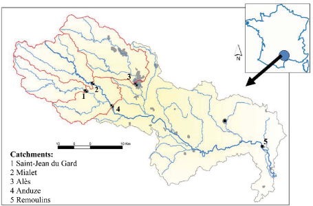
Figure 1. Hydrological map of the area of the Gardons, France (Neppel et al.,, 2010)

The geographic proximity of the four considered stations suggests dependence at high levels. This is visually confirmed by the pairwise plots in Figure 3, obtained after declustering (see Section 2).

The marginal data are classified into four different types, numbered from $0$ to $3$: ‘$0$’ denotes missing data, ‘$1$’ indicate an ‘exact’ record. Data of type ‘$2$’ are right-censored: the discharge is known to be greater than a given value. Finally, type ‘$3$’ data are left- and right-censored: the discharge is known to be comprised between a lower (possibly $0$) and an upper bound. Most data on the historical period are of type $3$. In the sequel, $j\ (1\leq j\leq d)$ denotes the location index and $t\ (1\leq t\leq n)$ is used for the the temporal one. A marginal observation $O_{j,t}$ is a $4$-uple $O_{j,t}=(\kappa_{j,t},Y_{j,t},L_{j,t},R_{j,t})\in\{0,1,2,3\}\times\mathbb{R}^{3}$, where $\kappa,Y,L$ and $R$ stand respectively for the data type, the recorded discharge (or some arbitrary value if $\kappa\neq 1$, which we denote NA), the lower bound (set to $0$ if missing), and the upper bound (set to $+\infty$ if missing).

2.2. Data pre-processing: extracting cluster maxima

Temporal dependence is handled by declustering, i.e. by fitting the model to cluster maxima instead of the raw daily data. The underlying assumption is that only short term dependence is present at extreme levels, so that excesses above high thresholds occur in clusters. Cluster maxima are treated as independent data to which a model for threshold excesses may be fitted. For an introduction to declustering techniques, the reader may refer to Coles, (2001) (Chap.5). For more details, see e.g. Leadbetter, (1983), or Davison and Smith, (1990) for applications when the quantities of interest are cluster maxima. Also, Ferro and Segers, (2003) propose a method for identifying the optimal cluster size, after estimating the extremal index. However, this latter approach relies heavily on ‘inter-arrival times’, which are not easily available in our context of censored data. In this study, we adopt a simple ‘run declustering’ approach, following Coles and Tawn, (1991) or Nadarajah, (2001) : a multivariate declustering threshold $\mathbf{v}=(v_{1},\dots v_{d})$ is specified (typically, $\mathbf{v}=(300,320,520,380)$ respectively for Saint-Jean, Mialet, Anduze and Alès), as well as a duration $\tau$ representative of the hydrological features of the catchment (typically $\tau=3$ days). Following common practice (Coles,, 2001), the thresholds are chosen in regions of stability of the maximum likelihood estimates of the marginal parameters.

In a censored data context, a marginal data $O_{j,t}$ exceeds $v_{j}$ (resp. is below $v_{j}$) if $\kappa_{j,t}=1$ and $Y_{j,t}>v_{j}$ (resp. $Y_{j,t}<v_{j}$), or if $\kappa_{j,t}\in\{2,3\}$ and $L_{j,t}>v_{j}$ (resp. $\kappa_{j,t}=3$ and $R_{j,t}<v_{j})$. If none of these conditions holds, we say that the data point has undetermined position with respect to the threshold. This is typically the case when some censoring intervals intersect the declustering thresholds whereas no coordinate is above threshold.

A cluster is initiated when at least one marginal observation $O_{j,t}$ exceeds the corresponding marginal threshold $v_{j}$. It ends only when, during at least $\tau$ successive days, all marginal observations are either below their corresponding threshold, or have undetermined position. Let $\{t_{i}\,,1\leq i\leq n_{\mathbf{v}}\}$ be the temporal indices of cluster starting dates. A cluster maximum $\mathbf{C}^{\vee}_{t_{i}}$ is the component-wise ‘maximum’ over a cluster duration $[{t_{i}},\dotsc,t_{i}+r]$. Its definition require special care in the context of censoring: the marginal cluster maximum is $C_{j,t_{i}}^{\vee}=\left(\kappa_{j,t_{i}}^{\vee},Y_{j,t_{i}}^{\vee},L_{j,t_{i}}^{\vee},R_{j,t_{i}}^{\vee}\right)$, with $Y_{j,t_{i}}^{\vee}=\max_{t_{i}\leq t\leq t_{i}+r}\{Y_{j,t}\}$ and similar definitions for $L_{j,t_{i}}^{\vee},R_{j,t_{i}}^{\vee}$. The marginal type $\kappa_{j,t_{i}}^{\vee}$ is that of the ‘largest’ record over the duration. More precisely, omitting the temporal index, if $Y_{j}^{\vee}>L_{j}^{\vee}$, then $\kappa_{j}^{\vee}=1$. Otherwise, if $L_{j}^{\vee}<R_{j}^{\vee}$, then $\kappa_{j}^{\vee}$ is set to $=3$; otherwise, if $L_{j}^{\vee}>0$, then $\kappa_{j}^{\vee}=2$ ; If none of the above holds, then the $j^{\text{th}}$ cluster coordinate is missing and $\kappa_{j}^{\vee}=0$.

Figure 2 shows the uni-variate projections of the multivariate declustering scheme, at each location. Points and segments below the declustering threshold indicate situations when the threshold was not exceeded at the considered location but at another one.

Anticipating Section 3, marginal cluster maxima below threshold are censored in the statistical analysis, so that their marginal types are always set to $3$, with lower bound at zero and upper bound at the threshold. This approach, fully described e.g. in Ledford and Tawn, (1996), prevents from having to estimate the marginal distribution below threshold, which does not participate in the dependence structure of extremes.

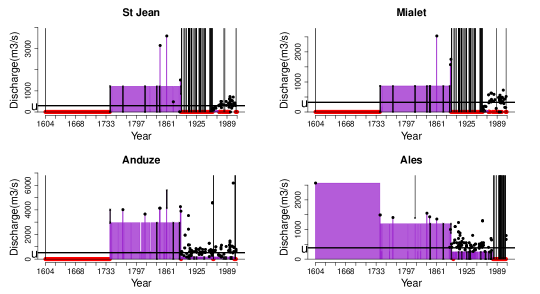
Figure 2. Extracted peaks-over-threshold at the four considered stations. Violet segments and areas represent data of type $2$ and $3$ available before declustering. Missing days are shown in red. Grey segments (resp. black points) are data of type 2 and 3 (resp. 1) belonging to an extracted multivariate cluster. The declustering threshold is represented by the horizontal black line. Vertical Grey lines are drawn at days which are missing at the considered location but which belong to a cluster, due to a threshold excess at another location.

After declustering and censoring below threshold, the data set is made of $n_{\mathbf{v}}=125$ $d$-variate cluster maxima $\{\mathbf{C}_{t_{i}}^{\vee},1\leq i\leq n_{v}\}$. The empirical mean cluster size is $\hat{\tau}=1.248$, which is to be used as a normalizing constant for the number of inter-cluster days. Namely, $m$ dependent inter-cluster observations contribute to the likelihood as $m/\hat{\tau}$ independent ones would do (see e.g. Beirlant et al., (2004), Chap. 10 or Coles, (2001), Chap. 8). As for those inter-cluster observations, $n_{\mathrm{bel}}=7562$ data points are below thresholds and only $9$ days are completely missing (no recording at any location). The remaining $n^{\prime}_{\mathbf{v}}=140\,674$ days are undetermined, and must be taken into account in the likelihood expression. They can be classified into $34$ homogeneous temporal blocks (i.e. all the days within a given block contain the same information), typically, between two recorded annual maxima. The block sizes are $n^{\prime}_{i}(1\leq i\leq 34)$, so that $\sum_{i=1}^{34}n^{\prime}_{i}=n^{\prime}_{\mathbf{v}}$.

Figure 3 shows bi-variate plots of the extracted cluster maxima together with undetermined blocks. Exact data are represented by points; One coordinate missing or censored yields a segment and censoring at both locations results in a rectangle. The plots show the asymmetrical nature of the problem under study: the quantity of available data varies from one pair to another (compare, e.g., the number of points available respectively for the pair Saint-Jean/Mialet and Saint-Jean/Alès). Joint modeling of excesses thus appears as a way of transferring information from one location to another. Also, the most extreme observations seem to occur simultaneously (by pairs): They are more numerous in the upper right corners than near the axes, which suggests the use of a dependence structure model for asymptotically dependent data such as the Dirichlet mixture (see Section 3.2).

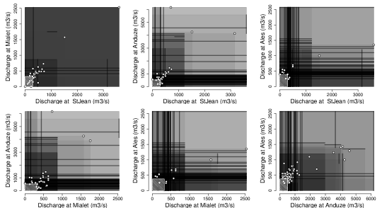
Figure 3. Bi-variate plots of the $124$ simultaneous stream-flow records (censored cluster maxima) at the four stations, and of the $34$ undetermined data blocks defined in section 2.2, over the whole period 1604-2010. Points represent exact data, gray lines and squares respectively represent data for which one (resp. two) coordinate(s) is (are) censored. Data superposition is represented by increased darkness. The striped rectangle at the origin is the region where all coordinates are below threshold.

3. Multivariate peaks-over-threshold model

This section provides a short description of the statistical model used for estimating the joint distribution of excesses above high thresholds. A more exhaustive statistical description is given in the above mentioned forthcoming paper. For an overview of statistical modeling of extremes in hydrology, the reader may refer e.g. to Katz et al., (2002). Also, Davison and Smith, (1990) focus on the uni-variate case and Coles and Tawn, (1991) review the most classical multivariate extreme value models.

3.1. Marginal model

After declustering, the extracted cluster maxima are assumed to be independent from each other. Their margins (values of the cluster maxima at each location considered separately) can be modeled by a Generalized Pareto distribution above threshold, provided that the latter is chosen high enough (Davison and Smith,, 1990; Coles,, 2001). Let $Y_{j,t_{i}}^{\vee}$ be the (possibly unobserved) maximum water discharge at station $j$, in cluster $i$ and let $F_{j}^{\mathbf{v}}$ the marginal cumulative distribution function (c.d.f.) below threshold. The marginal probability of an excess above threshold is denoted $\zeta_{j}\,\;(1\leq j\leq d)$. Following common practice (e.g. Coles and Tawn,, 1991; Davison and Smith,, 1990; Ledford and Tawn,, 1996), $\zeta_{j}$ is identified with its empirical estimate $\hat{\zeta}_{j}$, which is obtained as the proportion of intra-cluster days (after uni-variate declustering) among the non-missing days for the considered margin and threshold. For $\mathbf{v}$ as above, it yields $\boldsymbol{\zeta}\simeq(0.0021,0.0022,0.0022,0.0020)$.

The marginal models are thus

$$F_{j}^{(\xi_{j},\sigma_{j})}(y) =\mathbf{P}(Y_{j,t_{i}}^{\vee}<y|\xi_{j},\sigma_{j})\;,\qquad(1\leq j\leq d)$$

$$=\begin{cases}1-\zeta_{j}\left(1+\xi_{j}\frac{y-v_{j}}{\sigma_{j}}\right)^{-1/\xi}&(\text{if }y\geq v_{j}),\\ (1-\zeta_{j})F_{j}^{\mathbf{v}}(y)&(\text{if }y<v_{j}).\end{cases}$$

The marginal parameters are gathered into a $2d$-dimensional vector

$$\chi=\left(\log(\sigma_{1}),\dotsc,\log(\sigma_{d}),\xi_{1},\dotsc,\xi_{d}\right)\,,$$

and the uni-variate c.d.f.’s are denoted by $F_{j}^{\chi}$.

In a context of regional frequency analysis, it is further assumed that the shape parameter of the marginal GP distributions is identical for all catchments, i.e. $\xi_{1}=\dotsb=\xi_{d}$.

3.2. Dependence structure

In order to apply probabilistic results from multivariate extreme value theory, it is convenient to handle Fréchet distributed variables $X_{j,t_{i}}$, so that $P(X_{j,t_{i}}<x)=e^{-\frac{1}{x}},\;x>0$. This is achieved by defining a marginal transformation

$$\mathcal{T}_{j}^{\chi}(y)=-1/\log\left(F_{j}^{\chi}(y)\right),$$

and letting $X_{j,t_{i}}=\mathcal{T}_{j}^{\chi}(Y_{j,t_{i}})$. The dependence structure is then defined between the Fréchet-transformed data. One key assumption underlying multivariate extreme value models is that random vectors $\mathbf{Y}_{t}=(Y_{1,t},\dotsc,Y_{d,t})$ are regularly varying (see e.g. Resnick,, 1987, 2007; Beirlant et al.,, 2004; Coles and Tawn,, 1991). Multivariate regular variation (MRV) can be expressed as a radial homogeneity property of the distribution of the largest observations: For any region $A\subset(\mathbb{R}^{+})^{d}$ bounded away from $0$, if we denote $r.A=\{\mathbf{x}\in\mathbb{R}^{d}:\frac{1}{r}\mathbf{x}\in A\}$, then, for large $r_{0}$’s and for $r>r_{0}$, MRV and transformations to unit-Fréchet imply that

$$r\,\mathbf{P}(\mathbf{X}\in r.A)\underset{r_{0}\rightarrow\infty,r>r_{0}}{\sim}r_{0}\,\mathbf{P}(\mathbf{X}\in r_{0}.A)\,.$$ (1)

Switching to a pseudo-polar coordinates system, let $R=\sum_{j=1}^{d}X_{j}$ denote the radius and $\mathbf{W}=(\frac{X_{1}}{R},\dotsc,\frac{X_{d}}{R})$ denote the angular component of the Fréchet re-scaled data. In this context, $\mathbf{W}$ is a point on the simplex $\mathbf{S}_{d}$: $\sum_{j=1}^{d}W_{j}=1,\,W_{j}\geq 0$. Then (1) implies that, for any angular region $B\subset\mathbf{S}_{d}$,

$$\mathbf{P}(\mathbf{W}\in B\,|\,R>r_{0})\underset{r_{0}\rightarrow\infty}{\longrightarrow}H(B)$$ (2)

where $H$ is the so-called ‘angular probability measure’, i.e. the distribution of the angles corresponding to large radii. Since in addition, $\mathbf{P}(R>r_{0})\underset{r_{0}\rightarrow\infty}{\sim}\frac{d}{r_{0}}$, the joint behavior of large excesses is entirely determined by $H$.

As an illustration of this notion of angular distribution, Figure 4 shows two examples of simulated bi-variate data sets, with two different angular distributions and same Pareto-distributed radii. $H$’s density is represented by the pale red area. In the left panel, $H$ has most of its mass near the end points of the simplex (which is, in dimension 2, the segment $[(1,0),(0,1)]$, represented in blue on Figure 4) and the extremes are weakly dependent, so that events which are large in both components are scarce. In the limit case where $H$ is concentrated at the end-points of the simplex (not shown), the pair is said to be asymptotically independent. In contrast, the right panel shows a case of strong dependence: $H$ is concentrated near the middle point of the simplex and extremes occur mostly simultaneously.

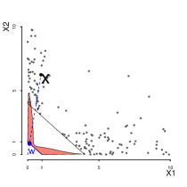
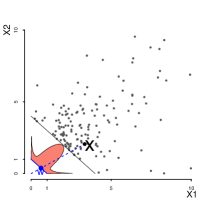
Figure 4. Two Examples of bivariate dependence structures of excesses above a radial threshold.
Grey points: simulated bivariate data. Pale red area: density of the angular distribution. Blue point: one randomly chosen angle $\mathbf{W}$, corresponding to the observation $\mathbf{X}$ (black point).

Contrary to the limit distribution of uni-variate excesses, $H$ does not have to belong to any particular parametric family. The only constraint on $H$ is due to the standard form of the $X_{j}$’s: $H$ is a valid angular distribution if and only if

$$\int_{\mathbf{S}_{d}}w_{j}\,\mathrm{d}H(\mathbf{w})=\frac{1}{d}\quad(1\leq j\leq d)\,.$$ (3)

In this paper, $H$ is chosen in the Dirichlet mixture model (Boldi and Davison,, 2007), which can approach any valid angular distribution. In short, a Dirichlet distribution with shape $\nu\in\mathbb{R}^{+}$ and center of mass $\boldsymbol{\mu}\in\mathbf{S}_{d}$ has density

$$\operatorname{diri}_{\nu,\boldsymbol{\mu}}(\mathbf{w})=\frac{\Gamma(\nu)}{\prod_{j=1}^{d}\Gamma(\nu\mu_{j})}\prod_{j=1}^{d}w_{j}^{\nu\mu_{j}-1}\,.$$

The density of a Dirichlet mixture distribution is therefore a weighted average of Dirichlet densities. A parameter for a $k$-mixture is thus of the form

$$\psi=\left((\mathit{p}_{1},\dotsc,\mathit{p}_{k}),(\boldsymbol{\mu}_{\,\cdot\,,1},\dotsc,\boldsymbol{\mu}_{\,\cdot\,,k}),(\nu_{1},\dotsc,\nu_{k})\right),$$

with weights $\mathit{p}_{m}>0$, $\sum_{m}\mathit{p}_{m}=1$, which will be denoted by $\psi=\left(\mathit{p}_{1:k},\boldsymbol{\mu}_{\,\cdot\,,1:k},\nu_{1:k}\right)$. The corresponding mixture density is

$$h_{\psi}(\mathbf{w})=\sum_{m=1}^{k}\mathit{p}_{m}\operatorname{diri}_{\nu,\boldsymbol{\mu}_{\,\cdot\,,m}}(\mathbf{w})\;.$$

As for the moment constraint (3), it is satisfied if and only if

$$\sum_{m=1}^{k}\mathit{p}_{m}\boldsymbol{\mu}_{\,\cdot\,,m}=\left(1/d,\dotsc,1/d\right)\,.$$ (4)

In other terms, the center of mass of the $\boldsymbol{\mu}_{\,\cdot\,,1:m}$’s, with weights $\mathit{p}_{1:m}$, must lie at the center of the simplex.

3.3. Estimation using censored data

Data censorship is the main technical issue in this paper. This section exposes the matter as briefly as possible. For the sake of readability, technical details and full statistical justification have been gathered in the above mentioned unpublished paper.

In order to account for censored data overlapping threshold and censored or missing components in the likelihood expression, it is convenient to write the model in terms of a Poisson point process, with intensity measure determined by $H$. More precisely, after marginal standardization, the time series of excesses above large thresholds can be described as a Poisson point process ($\operatorname{PRM}$),

$$\sum_{t=1}^{n}\mathds{1}_{\left(t,{\mathbf{X}_{t}}\right)}\sim\operatorname{PRM}(\,\mathrm{d}s\times\,\mathrm{d}\lambda)\quad\text{on }[0,n]\times A_{\boldsymbol{u}}\,,$$

where $n$ is the length of the observation period, $A_{\boldsymbol{u}}$ is the ‘extreme’ region on the Fréchet scale, $A_{\boldsymbol{u}}=[0,\infty]^{d}\setminus[0,u_{1}]\times\dotsb\times[0,u_{d}]$, above Fréchet thresholds $u_{j}=\mathcal{T}_{j}^{\chi}(v_{j})=-1/\log(1-\boldsymbol{\zeta}_{j})$. The notation $\,\mathrm{d}s$ stands for the Lebesgue measure on $[0,1]$ and $\lambda$ is the so-called ‘exponent measure’, which is related to the angular distribution’s density $h$ via

$$\frac{\,\mathrm{d}\lambda}{\,\mathrm{d}\mathbf{x}}(\mathbf{x})=d.h(\mathbf{w})r^{-(d+1)}\qquad\Big{(}r=\sum_{j=1}^{d}x_{j}\,,\,\mathbf{w}=\mathbf{x}/r\,\Big{)}\,.$$

This Poisson model has been widely used for statistical modeling of extremes (Coles,, 2001; Coles and Tawn,, 1991; Joe et al.,, 1992). The major advantage in our context is that it allows to take into account the undetermined data (which cannot be ascertained to be below nor above threshold), as they correspond to events of the kind

$$\mathbf{N}\left\{\left[{t^{\prime}_{i}},{t^{\prime}_{i}+n^{\prime}_{i}}\right]\times\left([0,\infty]^{d}\setminus[0,\mathcal{T}_{1}^{\chi}(R_{1,t^{\prime}_{i}})]\times\dotsc[0,\mathcal{T}_{d}^{\chi}(R_{d,t^{\prime}_{i}})]\right)\right\}=0\,,$$

where $\mathbf{N}\{\,\cdot\,\}$ is the number of points from the Poisson process in a given region.

In our context, $h$ is a Dirichlet mixture density: $h=h_{\psi}$. Let $\theta=\left(\chi,\psi\right)$ represent the parameter for the joint model, and $\lambda_{\psi}$ be the Poisson intensity associated with $h_{\psi}$. The likelihood in the Poisson model, in the absence of censoring, is

$$\mathcal{L}_{\mathbf{v}}\left(\{\mathbf{y}_{t}\}_{1\leq t\leq n},\theta\right) \propto e^{-n\,\lambda_{\psi}(A_{\boldsymbol{u}})}\prod_{i=1}^{n_{\mathbf{v}}}\Big{\{}\frac{\,\mathrm{d}\lambda_{\psi}}{\,\mathrm{d}\mathbf{x}}(\mathbf{x}_{t_{i}})\prod_{j:y_{j,t_{i}}>v_{j}}J_{j}^{\chi}(y_{j,t_{i}})\Big{\}}\,.$$ (5)

The $J_{j}^{\chi}$’s are the Jacobian terms accounting for the transformation $\mathbf{y}\to\mathbf{x}$.

The likelihood function in presence of such undetermined data and of censored data above threshold is obtained by integration of (5) in the direction of censorship. These integrals do not have a closed form expression. In a Bayesian context, a Markov Chain Monte-Carlo (MCMC) algorithm is built in order to sample from the posterior distribution, and the censored likelihood is involved at each iteration. Rather than using numerical approximations, whose bias may be difficult to assess, one option is to use a data augmentation framework (see e.g. Tanner and Wong,, 1987; Van Dyk and Meng,, 2001). The main idea is to draw the missing coordinates from their full conditional distribution in a Gibbs-step of the MCMC algorithm. Again, technicalities are omitted here.

4. Results

In this section, the multivariate extreme model with Dirichlet mixture dependence structure is fitted to the data from the Gardons, including all historical data and assuming a regional shape parameter. This regional hypothesis is confirmed (not rejected) by a likelihood ratio test: the p-value of the $\chi^{2}$ statistic is $0.16$. To assess the added value of taking into account historical data on the one hand, and of a regional analysis on the other hand, inference is also made without the regional shape assumption and considering only the systematic measurement period (starting from January, 1892). Thus, in total, four model fits are performed.

For each of the four experiments, $6$ chains of $10^{6}$ iterations are run in parallel, which requires a moderate computation time. Using parallel chains allows to check convergence using standard stationarity and mixing tests (Heidelberger and Welch, (1983)’s test , Gelman and Rubin, (1992)’s variance ratio test), available in the R statistical software. In the remainder of this section, all posterior predictive estimates are computed using the last $8\,10^{5}$ iterations of the chain obtaining the best stationarity score.

Figure 5 shows posterior histograms of the marginal parameters, together with the prior density. The posterior distributions are much more concentrated than the priors, indicating that marginal parameters are identifiable in each model. Also, the shape and scale panels are almost symmetric: a posterior distribution granting most weight to comparatively high shape parameters concentrates on comparatively low scales. This corroborates the fact that frequentist estimates of the shape and the scale parameter are negatively correlated (Ribereau et al.,, 2011). In the regional model as well as in the local one, the posterior variance of each parameter is reduced when taking into account historical data (except for the scale parameter at Anduze, for the local model). This confirms the general fact that taking into account more data tends to reduce the uncertainty of parameter estimates.

Shapes

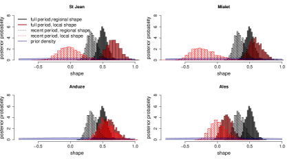
Scales

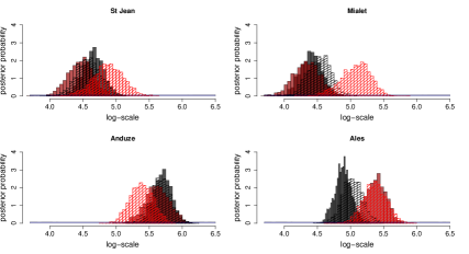
Figure 5. Prior and posterior distributions of the shape parameter (upper panel) and of the logarithm of the scale parameter (lower panel) at the four locations, estimated with or without historical data, in a regional framework or not.

Figure 6 shows posterior mean estimates of the return levels at each location, together with credible intervals based on posterior $0.05-0.95$ quantiles, in the four inferential frameworks. The return levels appear to be very sensitive to model choice: overall, taking into account the whole period increases the estimated return levels. In terms of mean estimate, the effect of imposing a global shape parameter varies from one station to another, as expected. For those return levels, the posterior credibility intervals seem to depend more on the mean return levels than on the choice of a regional or local framework. This seems at odds with the previous findings of reduced intervals for marginal parameters. However, one must note that the width of return level credibility intervals depends not only on that of the parameters, but also on the value of the mean estimates. Larger parameter estimates involve larger uncertainty in terms of return levels.

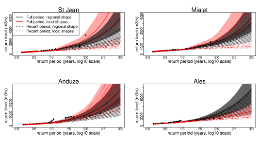
Figure 6. Return level plots at each location using four inferential frameworks with $90\%$ posterior quantiles. Dotted lines and hatched areas: data from he recent period only; Solid lines and shaded area: Full data set; Black lines and Grey area: Regional analysis, global shape parameter; Red lines and shaded red area: local shape parameters. Black (resp. Red) points: observed data plotted at the corresponding empirical return period using the whole (resp. recent) data set.

In addition to uni-variate quantities of interest such as marginal parameters or return level curves, having estimated the dependence structure gives access to multivariate quantities. Figure 7 shows the posterior mean estimates of the angular density. Since the four-variate version of the angular distribution cannot be easily represented, the bivariate marginal versions of the angular distribution are displayed instead. Here, the unit simplex (which was the diagonal blue segment in Figure 4) is represented by the horizontal axis, so that $H$ is a distribution function on $[0,1]$. As could be expected in view of Figure 3, extremes are rather strongly dependent. Moreover, the posterior distribution is overall well concentrated around the mean estimate.

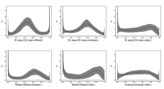
Figure 7. Posterior predictive bi-variate angular densities (black lines) with posterior $0.05-0.95$ quantiles (Grey areas).

The predictive angular distribution allows to estimate conditional probabilities of exceedance of high thresholds. As an example, figure 8 displays, for the six pairs $1\leq j<i\leq 4$, the posterior estimates of the conditional tail distribution functions $P(Y_{i}^{\vee}>y|Y_{j}^{\vee}>v_{j})$ at location $i$, conditioned upon an excess of the threshold $v_{j}$ at another location $j$. The predictive tail functions in the DM model concur with the empirical estimates for moderate values of $y$. For larger values, the empirical error grows and no empirical estimate exists outside the observed domain. However, the DM estimates are still defined and the size of the error region remains comparatively small.

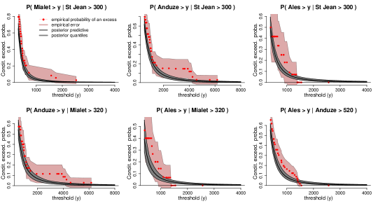
Figure 8. Conditional tail distributions. Black line and Grey area: posterior mean estimate and posterior $90\%$ credible intervals (posterior quantiles); red points: empirical tail function computed at the recorded points above threshold; pale red area: $90\%$ Gaussian confidence intervals around the empirical estimates.

Finally, one commonly used measure of dependence at asymptotically high levels between pairs of locations is defined by (Coles et al.,, 1999):

$$\boldsymbol{\chi}_{i,j}=\lim_{x\to\infty}\frac{P(X_{i}>x,X_{j}>x)}{P(X_{j}>x)}=\lim_{x\to\infty}P(X_{i}>x\left|X_{j}>x\right.)\,,$$

where $X_{i}$, $X_{j}$ are the Fréchet-transformed variables at locations $i$ and $j$. Since $X_{i}$ and $X_{j}$ are identically distributed, $\boldsymbol{\chi}_{i,j}=\boldsymbol{\chi}_{j,i}$. From its definition, $\boldsymbol{\chi}_{i,j}$ is comprised between $0$ and $1$; small values indicate weak dependence at high levels whereas values close to $1$ are characteristic of strong dependence. In the extreme case $\boldsymbol{\chi}=0$, the variables are asymptotically independent. In the case of Dirichlet mixtures, $\boldsymbol{\chi}_{i,j}$ has an explicit expression formed of incomplete Beta functions (Boldi and Davison,, 2007, eq. (9)). Figure 9 shows posterior box-plots of $\boldsymbol{\chi}$ for the six pairs. The strength of the dependence and the amount of uncertainty varies from one pair to another, but mean estimates are overall large (greater than $0.4$), indicating strong asymptotic dependence.

Figure 9. Dependence measure $\boldsymbol{\chi}_{i,j}$ for the six pairs of locations: Posterior box-plot.

In order to verify the consistency of those results with observed data, empirical quantities $P(X_{i}>x|X_{j}>x)$ have been computed and are displayed in Figure 10. More precisely, it is easy to see that

$$P(X_{i}>x|X_{j}>x)=P(Y_{i}^{\vee}>(F_{i}^{\chi})^{-1}\circ F_{j}^{\chi}(y)|Y_{j}^{\vee}>y)\,,$$

where $F_{i}^{\chi},F_{j}^{\chi}$ are the marginal cdf for location $i$ and $j$, and the $Y_{j}^{\vee},\,Y_{i}^{\vee}$’s are the observed data (cluster maxima). In Figure 10, the conditioning thresholds $y$ are the observed values of the conditioning variable $Y_{j}^{\vee}$ above the initial threshold $v_{j}$, of which the estimated return period (abscissa of the red points) is taken as its mean estimate using the marginal parameter components of the posterior sample. For each such $y$, $(F_{i}^{\chi})^{-1}\circ F_{j}^{\chi}(y)$ is estimated by its posterior mean value, again computed from the marginal posterior sample. Then, the conditional probability of an excess by $Y_{i}^{\vee}$ (Y-axis value of the red points) is computed empirically. In theory, as the return period increases, the red points should come closer to the horizontal black line, which is the mean estimate of $\boldsymbol{\chi}$ computed in the Dirichlet mixture dependence model, as in Figure 9. Note that in the Dirichlet model, the limiting value $\boldsymbol{\chi}$ is already reached at finite levels because the conditional probability of an excess on the Fréchet scale, $P(X_{i}>x|X_{j}>x)$, is constant in $x$. On the contrary, in an asymptoticallly independent model, the conditional exceeedance probability whould be decreasing towards zero. Results in Figure 10 are comforting: the mean values of $\boldsymbol{\chi}$ obtained from the Dirichet model are within the error regions of the empirical estimates. The latter are very large, compared to the posterior quantiles from the Dirichlet mixture, which illustrates the usefulness of an extreme value model for computing conditional probabilities of an excess.

This result has implications for computing the return periods of joint excesses of high thresholds. Consider, for example, the 10 years marginal return levels at two stations, $(q_{1},q_{2})$. If the excesses above these threhsolds were assumed to be independent, taking into account short term temporal dependence (the mean cluster size is $\tau=1.248$), the return period for the joint excess $(Y_{1}^{\vee}>q_{1},Y_{2}^{\vee}>q_{2})$ would be $10^{2}*(365/\tau)=29247.8$ years. On the contrary, accounting for spatial dependence, for example between the two first stations (St Jean and Mialet), yields an estimated return period for a joint excess of $10/\hat{\boldsymbol{\chi}}_{1,2}=10/0.645=15.5$ years.

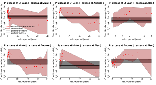
Figure 10. Observed conditional probability of exceedance of equally scaled thresholds. Red points: empirical estimates of conditional excesses; pale red regions, empirical standard error; horizontal black line and gray area, posterior mean and $0.05-0.95$ quantiles of the theoretical value in the DM model.

5. Discussion

This section lists the limitations of the model used in this paper and discusses directions for improvement.

5.1. Impact of systematic rating curve errors

The use of historical data allows extending the period of record and hence the availability of extreme flood events. However, historical data are also usually much more uncertain than recent systematic data, for two reasons: (i) the precision of historical water stages is limited; (ii) the transformation of these stage values into discharge values is generally based on a rating curve derived using a hydraulic model, which may induce large systematic errors.

The model used in the present paper ignores systematic errors (ii). This is because we focused on multivariate aspects through the use of the DM model to describe intersite dependence. However, systematic errors may have a non-negligible impact on marginal quantile estimates, as discussed by Neppel et al., (2010). Moreover, in a multivariate context, the impact of systematic errors on the estimation of the dependence structure is unclear at this stage and requires further evaluation. Future work will therefore aim at incorporating an explicit treatment of systematic errors, using models such as those discussed by Reis and Stedinger, (2005) or Neppel et al., (2010).

5.2. Comparing several models for intersite dependence

The DM model used in this paper to describe intersite dependence is a valid dependence model according to multivariate extreme value theory (MEVT). Many alternative approaches, not necessarily MEVT-compatible, have been proposed in the hydrological literature on regional estimation methods. Such approaches include simply ignoring dependence (e.g. Dalrymple,, 1960), the concept of ’equivalent number of sites’ (Reed et al.,, 1999) or the use of copulas (e.g. Renard,, 2011). This raises the question of the influence of the approach used to describe dependence on the following estimates:

• Marginal estimates, typically quantile estimates at each site. While the impact of ignoring dependence altogether has been studied by several authors (Stedinger,, 1983; Hosking and Wallis,, 1988; Madsen and Rosbjerg,, 1997; Renard and Lang,, 2007), the impact of alternative dependence models is less clear. In particular, since marginal estimates do not directly use the dependence model, it remains to be established whether or not different dependence models (e.g. asymptotically dependent vs. asymptotically independent) yield significantly different results.

• Joint or conditional estimates, as illustrated in Figures 3, 8 and 10 for instance. The dependence model obviously plays a much more important role in this case.

Such comparison has not been attempted in this paper because the use of censored historical data makes the application of standard methods like copulas much more challenging.

5.3. The treatment of intersite dependence in a highly dimensional context

As illustrated in the case study, the DM model is applicable in moderate dimension d=4. However, such semi-parametric approach is not geared toward highly-dimensional contexts (e.g. spatial rainfall using dozens or hundreds of rain gauges, or gridded data sets). Practical approaches for highly-dimensional multivariate extremes have been mostly proposed in the context of block maxima, using the theory of max-stable processes (De Haan,, 1984; Smith,, 1990; Schlather,, 2002; Westra and Sisson,, 2011). Estimation procedures e.g. using composite likelihood methods exist for such processes (Padoan et al.,, 2010), along with descriptive tools e.g. to define and estimate extremal dependence coefficients such as the madogram (Cooley et al.,, 2006). However, the development of models adapted to peaks-over-threshold is still an area of active research in a highly-dimensional spatial context and full modeling (which would e.g allow simulation of joint excesses) remain elusive. Recent theoretical advances (Ferreira and de Haan,, 2012; Dombry and Ribatet,, 2013) give cause to hope for, and expect, future development of spatial peaks-over-threshold models.

6. Conclusion

This paper illustrates the use of a multivariate peaks-over-threshold model to combine regional estimation and historical floods. This model is based on a semi-parametric Dirichlet Mixture to describe intersite dependence, while Generalized Pareto distributions are used for margins. A data augmentation scheme is used to enable the inclusion of censored historical flood data. The model is applied to four catchments in Southern France where historical flood data are available.

The first objective of this case study was to assess the relative impact of regional and historical information on marginal quantile estimates at each site. The main results can be summarized as follows:

• Over the four considered versions of the model, the version ignoring historical floods and performing local estimation yields estimates that may strongly differ from the other versions. The three other versions (which either use historical floods or perform regional estimation or both) yield more consistent estimates. This illustrates the benefit of extending the at-site sample using either historical or regional information, or both.

• Compared with the most complete version of the model (which enables both historical floods and regional estimation), the version only implementing regional estimation (but ignoring historical floods) yields smaller estimates of the shape parameter, and hence smaller quantiles. This result is likely specific to this particular data set, for which many large floods have been recorded during the historical period.

• Compared with the most complete version of the model, the version using historical floods but implementing local estimation yields higher quantiles for three catchments but lower quantiles on the fourth.

• The uncertainty in parameter estimates generally decreases when more information (regional, historical or both) is included in the inference. However, this does not necessarily result in smaller uncertainty in quantile estimates. This is because this uncertainty does not only depends on the uncertainty in parameter estimates, but also on the value taken by the parameters. In particular, a precise but large shape parameter may result in more uncertain quantiles than a more imprecise but lower shape parameter.

The second objective was to investigate the nature of asymptotic dependence in this flood data set, by taking advantage of the existence of extremely high joint exceedances in the historical data. Results in terms of predictive angular density suggest the existence of such dependence between every pairs of catchments of asymmetrical nature: some pairs are more dependent than others at asymptotic levels. In addition, the Dirichlet Mixture model allows to compute bi-variate conditional probabilities of large threshold exceedances, which are poorly estimated with empirical methods. The limiting values of the conditional probabilities, theoretically obtained with increasing thresholds, are substantially non zero (they range between $0.4$ and $0.65$), which confirms the strength and the asymmetry of pairwise asymptotic dependence for this data set and induces multivariate return periods much shorter than they would be in the asymptotically independent case.

7. Acknowledgement

The first author would like to thank Anne-Laure Fougères and Philippe Naveau for their useful advice. Part of this work has been supported by the EU-FP7 ACQWA Project (www.acqwa.ch), by the PEPER-GIS project, by the ANR (MOPERA, McSim, StaRMIP) and by the MIRACCLE-GICC project.

References

- Beirlant et al., (2004) Beirlant, J., Goegebeur, Y., Segers, J., and Teugels, J. (2004). Statistics of extremes: Theory and applications. John Wiley & Sons: New York.
- Boldi and Davison, (2007) Boldi, M.-O. and Davison, A. C. (2007). A mixture model for multivariate extremes. Journal of the Royal Statistical Society: Series B (Statistical Methodology), 69(2):217–229.
- Coles, (2001) Coles, S. (2001). An introduction to statistical modeling of extreme values. Springer Verlag.
- Coles et al., (1999) Coles, S., Heffernan, J., and Tawn, J. A. (1999). Dependence measures for extreme value analyses. Extremes, 2:339–365.
- Coles and Tawn, (1991) Coles, S. and Tawn, J. (1991). Modeling extreme multivariate events. JR Statist. Soc. B, 53:377–392.
- Cooley et al., (2006) Cooley, D., Naveau, P., and Poncet, P. (2006). Variograms for spatial max-stable random fields. In Dependence in probability and statistics, pages 373–390. Springer.
- Dalrymple, (1960) Dalrymple, T. (1960). Flood frequency analyses. Water-supply paper 1543-A.
- Davison and Smith, (1990) Davison, A. and Smith, R. (1990). Models for exceedances over high thresholds. Journal of the Royal Statistical Society. Series B (Methodological), pages 393–442.
- De Haan, (1984) De Haan, L. (1984). A spectral representation for max-stable processes. The annals of probability, pages 1194–1204.
- De Haan and De Ronde, (1998) De Haan, L. and De Ronde, J. (1998). Sea and wind: Multivariate extremes at work. Extremes, 1:7–45.
- Dombry and Ribatet, (2013) Dombry, C. and Ribatet, M. (2013). Functional regular variations, pareto processes and peaks over threshold.
- Ferreira and de Haan, (2012) Ferreira, A. and de Haan, L. (2012). The generalized pareto process; with a view towards application and simulation. arXiv preprint arXiv:1203.2551v2.
- Ferro and Segers, (2003) Ferro, C. and Segers, J. (2003). Inference for clusters of extreme values. Journal of the Royal Statistical Society: Series B (Statistical Methodology), 65(2):545–556.
- Gaume et al., (2010) Gaume, E., Gaal, L., Viglione, A., Szolgay, J., Kohnova, S., and Bloschl, G. (2010). Bayesian mcmc approach to regional flood frequency analyses involving extraordinary flood events at ungauged sites. Journal of Hydrology, 394:101–117.
- Gelman and Rubin, (1992) Gelman, A. and Rubin, D. (1992). Inference from iterative simulation using multiple sequences. Statistical science, pages 457–472.
- Gumbel, (1960) Gumbel, E. (1960). Distributions des valeurs extrêmes en plusieurs dimensions. Publ. Inst. Statist. Univ. Paris, 9:171–173.
- Heidelberger and Welch, (1983) Heidelberger, P. and Welch, P. (1983). Simulation run length control in the presence of an initial transient. Operations Research, pages 1109–1144.
- Hosking, (1985) Hosking, J. (1985). Maximum-likelihood estimation of the parameters of the generalized extreme-value distribution. Applied Statistics, 34:301–310.
- Hosking and Wallis, (1987) Hosking, J. and Wallis, J. R. (1987). Parameter and quantile estimation for the generalized pareto distribution. Technometrics, 29(3):339–349.
- Hosking and Wallis, (1988) Hosking, J. and Wallis, J. R. (1988). The effect of intersite dependence on regional flood frequency analysis. Water Resources Research, 24:588–600.
- Hosking and Wallis, (1997) Hosking, J. and Wallis, J. R. (1997). Regional Frequency Analysis: an approach based on L-Moments. Cambridge University Press, Cambridge, UK.
- Jin and Stedinger, (1989) Jin, M. and Stedinger, J. R. (1989). Flood frequency analysis with regional and historical information. Water Resources Research, 25(5):925–936.
- Joe et al., (1992) Joe, H., Smith, R. L., and Weissman, I. (1992). Bivariate threshold methods for extremes. Journal of the Royal Statistical Society. Series B (Methodological), pages 171–183.
- Katz et al., (2002) Katz, R. W., Parlange, M. B., and Naveau, P. (2002). Statistics of extremes in hydrology. Advances in water resources, 25(8):1287–1304.
- Lang et al., (1999) Lang, M., Ouarda, T., and Bobee, B. (1999). Towards operational guidelines for over-threshold modeling. Journal of Hydrology, 225:103–117.
- Leadbetter, (1983) Leadbetter, M. (1983). Extremes and local dependence in stationary sequences. Probability Theory and Related Fields, 65(2):291–306.
- Ledford and Tawn, (1996) Ledford, A. and Tawn, J. (1996). Statistics for near independence in multivariate extreme values. Biometrika, 83(1):169–187.
- (28) Madsen, H., Pearson, C. P., and Rosbjerg, D. (1997a). Comparison of annual maximum series and partial duration series methods for modeling extreme hydrologic events .2. regional modeling. Water Resources Research, 33(4):759–769.
- (29) Madsen, H., Rasmussen, P. F., and Rosbjerg, D. (1997b). Comparison of annual maximum series and partial duration series methods for modeling extreme hydrologic events .1. at-site modeling. Water Resources Research, 33(4):747–757.
- Madsen and Rosbjerg, (1997) Madsen, H. and Rosbjerg, D. (1997). The partial duration series method in regional index-flood modeling. Water Resources Research, 33(4):737–746.
- Nadarajah, (2001) Nadarajah, S. (2001). Multivariate declustering techniques. Environmetrics, 12(4):357–365.
- Naulet et al., (2005) Naulet, R., Lang, M., Ouarda, T. B., Coeur, D., Bobée, B., Recking, A., and Moussay, D. (2005). Flood frequency analysis on the ardèche river using french documentary sources from the last two centuries. Journal of Hydrology, 313(1):58–78.
- Neppel et al., (2010) Neppel, L., Renard, B., Lang, M., Ayral, P., Coeur, D., Gaume, E., Jacob, N., Payrastre, O., Pobanz, K., and Vinet, F. (2010). Flood frequency analysis using historical data: accounting for random and systematic errors. Hydrological Sciences Journal–Journal des Sciences Hydrologiques, 55(2):192–208.
- O’Connel et al., (2002) O’Connel, D., Ostenaa, D., Levish, D., and Klinger, R. (2002). Bayesian flood frequency analysis with paleohydrologic bound data. Water Resources Research, 38(5).
- Padoan et al., (2010) Padoan, S. A., Ribatet, M., and Sisson, S. A. (2010). Likelihood-based inference for max-stable processes. Journal of the American Statistical Association, 105(489).
- Parent and Bernier, (2003) Parent, E. and Bernier, J. (2003). Bayesian pot modeling for historical data. Journal of hydrology, 274:95–108.
- Payrastre et al., (2011) Payrastre, O., Gaume, E., and Andrieu, H. (2011). Usefulness of historical information for flood frequency analyses: Developments based on a case study. Water Resources Research, 47.
- Reed et al., (1999) Reed, D. W., Faulkner, D. S., and Stewart, E. J. (1999). The forgex method of rainfall growth estimation - ii: Description. Hydrology and Earth System Sciences, 3(2):197–203.
- Reis and Stedinger, (2005) Reis, D. and Stedinger, J. R. (2005). Bayesian mcmc flood frequency analysis with historical information. Journal of Hydrology, 313(1-2):97–116.
- Renard, (2011) Renard, B. (2011). A bayesian hierarchical approach to regional frequency analysis. Water Resources Research, 47.
- Renard and Lang, (2007) Renard, B. and Lang, M. (2007). Use of a gaussian copula for multivariate extreme value analysis: some case studies in hydrology. Advances in Water Resources, 30(4):897–912.
- Resnick, (1987) Resnick, S. (1987). Extreme values, regular variation, and point processes, volume 4 of Applied Probability. A Series of the Applied Probability Trust. Springer-Verlag, New York.
- Resnick, (2007) Resnick, S. (2007). Heavy-Tail Phenomena: Probabilistic and Statistical Modeling. Springer Series in Operations Research and Financial Engineering.
- Ribereau et al., (2011) Ribereau, P., Naveau, P., and Guillou, A. (2011). A note of caution when interpreting parameters of the distribution of excesses. Advances in Water Resources, 34(10):1215–1221.
- Sabourin, (2014) Sabourin, A. (2014). Semi-parametric modeling of excesses above high multivariate thresholds with censored data. submitted.
- Sabourin and Naveau, (2013) Sabourin, A. and Naveau, P. (2013). Bayesian dirichlet mixture model for multivariate extremes: A re-parametrization. Computational Statistics & Data Analysis, DOI 10.1016/j.csda.2013.04.021.
- Schlather, (2002) Schlather, M. (2002). Models for stationary max-stable random fields. Extremes, 5(1):33–44.
- Smith, (1994) Smith, R. (1994). Multivariate threshold methods. Extreme Value Theory and Applications, 1:225–248.
- Smith et al., (1997) Smith, R., Tawn, J., and Coles, S. (1997). Markov chain models for threshold exceedances. Biometrika, 84(2):249–268.
- Smith, (1990) Smith, R. L. (1990). Max-stable processes and spatial extremes. Unpublished manuscript, Univer.
- Stedinger, (1983) Stedinger, J. R. (1983). Estimating a regional flood frequency distribution. Water Resources Research, 19:503–510.
- Stedinger and Cohn, (1986) Stedinger, J. R. and Cohn, T. A. (1986). Flood frequency-analysis with historical and paleoflood information. Water Resources Research, 22(5):785–793.
- Stephenson, (2003) Stephenson, A. (2003). Simulating multivariate extreme value distributions of logistic type. Extremes, 6(1):49–59.
- Stephenson, (2009) Stephenson, A. (2009). High-dimensional parametric modelling of multivariate extreme events. Australian & New Zealand Journal of Statistics, 51(1):77–88.
- Tanner and Wong, (1987) Tanner, M. and Wong, W. (1987). The calculation of posterior distributions by data augmentation. Journal of the American Statistical Association, 82(398):528–540.
- Tasker and Stedinger, (1987) Tasker, G. D. and Stedinger, J. R. (1987). Regional regression of flood characteristics employing historical information. Journal of Hydrology, 96:255–264.
- Tasker and Stedinger, (1989) Tasker, G. D. and Stedinger, J. R. (1989). An operational gls model for hydrologic regression. Journal of Hydrology, 111:361:375.
- Van Dyk and Meng, (2001) Van Dyk, D. and Meng, X. (2001). The art of data augmentation. Journal of Computational and Graphical Statistics, 10(1):1–50.
- Westra and Sisson, (2011) Westra, S. and Sisson, S. A. (2011). Detection of non-stationarity in precipitation extremes using a max-stable process model. Journal of Hydrology, 406(1):119–128.