Approximation of Eigenfunctions in Kernel-based Spaces

Abstract

Kernel-based methods in Numerical Analysis have the advantage of yielding optimal recovery processes in the ”native” Hilbert space $\mathcal{H}$ in which they are reproducing. Continuous kernels on compact domains have an expansion into eigenfunctions that are both $L_{2}$-orthonormal and orthogonal in $\mathcal{H}$ (Mercer expansion). This paper examines the corresponding eigenspaces and proves that they have optimality properties among all other subspaces of $\mathcal{H}$. These results have strong connections to $n$-widths in Approximation Theory, and they establish that errors of optimal approximations are closely related to the decay of the eigenvalues.

Though the eigenspaces and eigenvalues are not readily available, they can be well approximated using the standard $n$-dimensional subspaces spanned by translates of the kernel with respect to $n$ nodes or centers. We give error bounds for the numerical approximation of the eigensystem via such subspaces. A series of examples shows that our numerical technique via a greedy point selection strategy allows to calculate the eigensystems with good accuracy.

Keywords: Mercer kernels, radial basis functions, eigenfunctions, eigenvalues, $n$-widths, optimal subspaces, greedy methods
2000 MSC: 41Axx, 41A46, 41A58, 42Cxx, 42C15, 42A82, 45P05, 46E22, 47A70, 65D05, 65F15, 65R10, 65T99

1 Introduction

We start with a few background facts about kernel-based methods. Details can be retrieved from the monographs [2, 27, 7] and the surveys [1, 25]. Let $\Omega\subset\mathbb{R}^{d}$ be a nonempty set, and let $K:\Omega\times\Omega\to\mathbb{R}$ be a positive definite and symmetric kernel on $\Omega$. Associated with $K$ there is a unique native space $\mathcal{H}(\Omega)$, that is a separable Hilbert space of functions $f:\Omega\to\mathbb{R}$ where K is the reproducing kernel. This means that $K(\cdot,x)$ is the Riesz representer of the evaluation functional $\delta_{x}$, i.e.,

$$f(x)=(f,K(\cdot,x)),\;\;\hbox{ for all }x\in\Omega,\;f\in\mathcal{H}(\Omega)$$ (1)

where we use the notation $(\cdot,\cdot)$, without subscript, to denote here and in the following the inner product of $\mathcal{H}(\Omega)$. Also the converse holds: any Hilbert space on $\Omega$ where the evaluation functionals $\delta_{x}$ are continuous for any $x\in\Omega$ is the native space of a unique kernel.

One way to construct the native space is as follows. First one considers the space $\mathcal{H}_{0}(\Omega)=\text{span}\{K(\cdot,x),x\in\Omega\}$ and then equips it with the positive definite and symmetric bilinear form

$$\left(\sum_{j}c_{j}K(\cdot,x_{j}),\sum_{i}d_{i}K(\cdot,x_{i})\right):=\sum_{j,i}c_{j}d_{i}K(x_{j},x_{i}).$$

The native space $\mathcal{H}(\Omega)$ then is the closure of $\mathcal{H}_{0}(\Omega)$ with respect to the inner product defined by this form.

Given a finite set $X_{n}=\{x_{1},\dots,x_{n}\}\subset\Omega$ of distinct points, the interpolant $s_{f,X_{n}}$ of a function $f\in\mathcal{H}(\Omega)$ on $X_{n}$ is uniquely defined, since the kernel matrix

$$A=[K(x_{i},x_{j})]_{i,j=1}^{n}$$

is positive definite, the kernel being positive definite. Letting $V(X_{n})\subset\mathcal{H}(\Omega)$ be the subspace spanned by the kernel translates $K(\cdot,x_{1})$, $\dots$, $K(\cdot,x_{n})$, the interpolant $s_{f,X_{n}}$ is the projection of $f$ into $V(X_{n})$ with respect to $(\cdot,\cdot)$.

The usual way to study the approximation error is to consider the Power Function $P_{n}(x)$ of $X_{n}$ at $x$, that is the $\mathcal{H}(\Omega)$-norm of the pointwise error functional $f\mapsto f(x)-s_{f,X_{n}}(x)$ at $x$, but we will consider also other measurements of the interpolation error, and other projectors.

We make the additional assumptions that $\Omega$ is a compact set in $\mathbb{R}^{d}$ and the kernel is continuous on $\Omega\times\Omega$. This ensures that the native space has a continuous embedding into $L_{2}(\Omega)$. Indeed, using the reproducing property (1) we have

$$\|f\|_{L_{2}}\leq\left(\int_{\Omega}K(x,x)dx\right)^{1/2}\|f\|\;\;\hbox{ for all }f\in\mathcal{H}(\Omega)$$

where the integral of the kernel is finite. This allows to define a compact and self-adjoint integral operator $T:L_{2}(\Omega)\to L_{2}(\Omega)$ which will be crucial for our goals. For $f\in L_{2}(\Omega)$ we define

$$Tf(x)=\int_{\Omega}K(x,y)f(y)dy,\;\;x\in\Omega.$$ (2)

It can be shown that the range $T(L_{2}(\Omega))$ of $T$ is dense in $\mathcal{H}(\Omega)$, and

$$(f,g)_{L_{2}}=(f,Tg)\text{ for all }f\in\mathcal{H}(\Omega),\;g\in L_{2}(\Omega).$$ (3)

Remark 1.

The operator $T$ can be defined using any positive and finite measure $\mu$ with full support on $\Omega$ (see [26]) and the same properties still hold, but we will concentrate here on the Lebesgue measure.

The following theorem (see e.g. [20, Ch. 5]) applies to our situation, and provides a way to represent the kernel as an expansion (or Hilbert - Schmidt or Mercer) kernel (see e.g. [23, 22]).

Theorem 2 (Mercer).

If $K$ is a continuous and positive definite kernel on a compact set $\Omega$, the operator $T$ has a countable set of positive eigenvalues $\lambda_{1}\geq\lambda_{2}\geq\dots>0$ and eigenfunctions $\{\varphi_{j}\}_{j\in\mathbb{N}}$ with $T\varphi_{j}=\lambda_{j}\varphi_{j}$. The eigenfunctions are orthonormal in $L_{2}(\Omega)$ and orthogonal in $\mathcal{H}(\Omega)$ with $\|\varphi_{j}\|=\lambda_{j}^{-1}$. Moreover, the kernel can be decomposed as

$$K(x,y)=\sum_{j=1}^{\infty}\lambda_{j}\ \varphi_{j}(x)\ \varphi_{j}(y)\;\;\;x,y\in\Omega,$$ (4)

where the sum is absolutely and uniformly convergent.

From now on we will call $\{\sqrt{\lambda_{j}}\varphi_{j}\}_{j\in\mathbb{N}}$ the eigenbasis, and use the notation $E_{n}=\text{span}\{\sqrt{\lambda_{j}}\varphi_{j},j=1,\dots,n\}$.

We recall that it is also possible to go the other way round and define a positive definite and continuous kernel starting from a given sequence of functions $\{\varphi_{j}\}_{j}$ and weights $\{\lambda_{j}\}_{j}$, provided some mild conditions of summability and linear independence. See [23] for a detailed discussion about this construction, and note that eigenfunction expansions play a central role in the RBF-QR technique dealt with in various papers [8, 6] recently. Furthermore, eigenexpansion techniques are a central tool when working with kernels on spheres and Riemannian manifolds [5, 12, 16, 9].

In this paper we shall study the eigenbasis in detail and compare the eigenspaces to other $n$-dimensional subspaces of $\mathcal{H}(\Omega)$. General finite dimensional subspaces and their associated $L_{2}(\Omega)$- and $\mathcal{H}(\Omega)$- projectors are treated in Section 2. In particular, the approximation error is bounded in terms of generalized Power Functions that turn out to be very useful for the rest of the paper. The determination of error-optimal $n$-dimensional subspaces is the core of Section 3, and is treated there by $n$-widths, proving that eigenspaces are optimal under various circumstances. In addition to the case of Kolmogorov $n$-width as treated in [23], we prove that eigenspaces minimize the $L_{2}(\Omega)$ norm of the Power Function.

In Section 4 we move towards numerical calculation of eigenbases by focusing on (possibly finite-dimensional) closed subspaces. In particular, we want to use subspaces $V(X_{n})$ spanned by kernel translates $K(\cdot,x_{1})$, $\dots$, $K(\cdot,x_{n})$ for point sets $X_{n}$ to calculate approximations to the eigenbasis. By means of Power Functions we can bound the error committed by working with finite dimensional subspaces.

Section 5 focuses on the decay of eigenvalues. We recall the fact that increased smoothness of the kernel leads to faster decay of eigenvalues. We prove that using point-based subspaces $V(X_{n})$ we can approximate the first $n$ eigenvalues with an error connected to the decay of $\lambda_{n}$.

Section 6 describes the numerical algorithms used for the examples in Section 7. In particular, we use a greedy method for selecting sets $X_{n}$ of $n$ points out of $N$ given points such that eigenvalue calculations in $V(X_{n})$ are stable and efficient.

Finally, Section 7 shows that our algorithm allows to approximate the eigenvalues for Sobolev spaces in a way that recovers the true decay rates, and by results of Section 5 we have bounds on the committed error. For Brownian bridge kernels the eigenvalues are known, and our algorithm approximates them very satisfactorily.

2 Projectors

As mentioned in the introduction, the interpolation problem in $\mathcal{H}(\Omega)$ is well defined, and the interpolation operator is a $\mathcal{H}(\Omega)$-projector into the spaces generated by translates of the kernel. But we want to look also at fully general subspaces $V_{n}$ of $\mathcal{H}(\Omega)$, generated by any set of $n$ basis functions, and at other linear approximation processes defined on such spaces, e.g. approximations in the $L_{2}(\Omega)$ norm.

For instance, we consider the two projectors

$$\begin{array}[]{rcll}\Pi_{L_{2},V_{n}}f&=&\sum_{j=1}^{n}(f,w_{j})_{L_{2}}w_{j},&f\in\mathcal{H}(\Omega),\\ \Pi_{\mathcal{H},V_{n}}f&=&\sum_{j=1}^{n}(f,v_{j})v_{j},&f\in\mathcal{H}(\Omega),\end{array}$$

where the $w_{j}$ and $v_{j}$ are $L_{2}(\Omega)$- and $\mathcal{H}(\Omega)$- orthonormal basis functions of $V_{n}$, respectively. The first projector is defined on all of $L_{2}(\Omega)$ and can be analyzed on all intermediate spaces. We want to see how these projectors are connected.

The two projectors do not coincide in general, but there is a special case. For the sake of clarity we present here the proof of the following Lemma, even if it relies on a result that is proven in Section 4.

Lemma 3.

If the projectors coincide on $\mathcal{H}(\Omega)$ for an $n$-dimensional space $V_{n}$, then $V_{n}$ is spanned by $n$ eigenfunctions. The converse also holds.

Proof.

We start with the converse. For each fixed $\varphi_{j}$, thanks to (3), we have

$$(f,\varphi_{j})_{L_{2}}={\lambda_{j}}(f,\varphi_{j})\text{ for all }f\in\mathcal{H}(\Omega).$$

Then

$$\Pi_{L_{2},V_{n}}f= \sum_{j=1}^{n}(f,\varphi_{j})_{L_{2}}\varphi_{j}=\sum_{j=1}^{n}{\lambda_{j}}(f,\varphi_{j})\varphi_{j}$$

$$= \sum_{j=1}^{n}(f,\sqrt{\lambda_{j}}\varphi_{j})\sqrt{\lambda_{j}}\varphi_{j}=\Pi_{\mathcal{H},V_{n}}f.$$

Assume now that the projectors coincide on $\mathcal{H}(\Omega)$. We can choose a basis $\{v_{j}\}_{j}$ of $V_{n}$ which is $L_{2}(\Omega)$-orthonormal and $\mathcal{H}(\Omega)$-orthogonal (see Lemma 10), with $\|v_{j}\|^{2}=1/\sigma_{j}$. Since $\Pi_{L_{2},V_{n}}f=\Pi_{\mathcal{H},V_{n}}f$ for any $f\in\mathcal{H}(\Omega)$, necessarily

$$(f,v_{j})_{L_{2}}={\sigma_{j}}(f,v_{j})\text{ for all }f\in\mathcal{H}(\Omega)\text{ and }j=1,\dots,n,$$

and in particular for $f=K(\cdot,x)$, $x\in\Omega$. Consequently, $\{v_{j}\}_{j}$ and $\{\sigma_{j}\}_{j}$ are eigenfunctions / eigenvalues of $T$. ∎

We are now interested in an error analysis of the approximation by functions from these general subspaces, and we want to allow both of the above projectors.

Definition 4.

For a normed linear space $H$ of functions on $\Omega$ and a linear operator $\Pi$ on $H$ such that all the functionals $\delta_{x}-\delta_{x}\circ\Pi$ are continuous for some norm $\|\cdot\|_{H}$, the generalized Power Function in $x\in\Omega$ is the norm of the error functional at $x$, i.e.,

$$P_{\Pi,\|.\|_{H}}(x):=\sup_{\|f\|_{H}\leq 1}|f(x)-(\Pi f)(x)|.$$ (5)

The definition fits our situation, because we are free to take $\Pi=\Pi_{\mathcal{H},V_{n}}$ with $\|.\|_{H}=\|.\|$, the normed linear space $H$ being $\mathcal{H}(\Omega)$.

In the following, when no confusion is possible, we will use the simplified notation $P_{V_{n},\mathcal{H}}$ or just $P_{V_{n}}$ to denote the Power Function of $\Pi_{\mathcal{H},V_{n}}$ with respect to $\|\cdot\|$.

To look at the relation between generalized Power Functions, subspaces and bases we start with the following lemma.

Lemma 5.

If a separable Hilbert space $H$ of functions on $\Omega$ has continuous point evaluation, then each $H$-orthonormal basis $\{v_{j}\}_{j}$ satisfies

$$\sum_{j}v_{j}^{2}(x)<\infty.$$

Conversely, the above condition ensures that all point evaluation functionals are continuous.

Proof.

The formula

$$f=\displaystyle{\sum_{j}(f,v_{j})_{H}v_{j}}$$

holds in the sense of limits in $H$. If point evaluations are continuous, we can write

$$f(x)=\displaystyle{\sum_{j}(f,v_{j})_{H}v_{j}(x)\text{ for all }x\in\Omega}$$

in the sense of limits in $\mathbb{R}$. Since the sequence $\{(f,v_{j})_{H}\}_{j}$ is in $\ell_{2}$ and can be an arbitrary element of that space, the sequence $\{v_{j}(x)\}_{j}$ must be in $\ell_{2}$, because the above expression is a continuous linear functional on $\ell_{2}$.

For the converse, observe that for any $n\in\mathbb{N}$, $x\in\Omega$ and $\sum_{j=1}^{n}c_{j}^{2}\leq 1$ the term $\sum_{j=1}^{n}c_{j}v_{j}(x)$ is bounded above by $\sum_{j}v_{j}^{2}(x)$, which is finite for any $x\in\Omega$. Hence, for any $x\in\Omega$, $\sup_{\|f\|_{H}\leq 1}|f(x)|$ is uniformly bounded for $f\in H$. ∎

Lemma 6.

For projectors $\Pi_{V_{n}}$ within separable Hilbert spaces $H$ of functions on some domain $\Omega$ onto finite-dimensional subspaces $V_{n}$ generated by $H$-orthonormal functions $v_{1},\ldots,v_{n}$ that are completed, we have

$$P^{2}_{\Pi_{V_{n}},\|.\|_{H}}(x)=\sum_{k>n}v_{k}^{2}(x)$$

provided that all point evaluation functionals are continuous.

Proof.

The pointwise error at $x$ is

$$f(x)-\Pi_{V_{n}}f(x) =\sum_{k>n}(f,v_{k})_{H}v_{k}(x),$$

and, thanks to the previous Lemma, we can safely bound its norm as

$$|f(x)-\Pi_{V_{n}}f(x)|^{2} \leq\sum_{k>n}(f,v_{k})_{H}^{2}\sum_{j>n}v_{j}^{2}(x)$$

$$=\|f-\Pi_{V_{n}}f\|_{H}^{2}\sum_{j>n}v_{j}^{2}(x)\leq\|f\|_{H}^{2}\sum_{j>n}v_{j}^{2}(x),$$

with equality if $f\in V_{n}^{\perp}$. ∎

This framework includes also the usual Power Function.

Lemma 7.

Let $X_{n}$ be a set of $n$ points in a compact domain $\Omega$, and let $V(X_{n})$ be spanned by the $X_{n}$-translates of $K$. Then the above notion of $P_{V(X_{n})}$ coincides with the standard notion of the interpolatory Power Function wrt. $X_{n}$.

The proof follows from the fact that the interpolation operator coincides with the projector $\Pi_{\mathcal{H},V(X_{n})}$ and the Power Function is in both cases defined as the norm of the pointwise error functional.

3 Minimal error subspaces

In this section we present the main results of this paper. Our goal is to analyze the behavior of the approximation error, considered from different points of view, depending on the $n$-dimensional subspace $V_{n}$. Roughly speaking, we will see that it is possible to exactly characterize the $n$-dimensional subspaces of minimal error, both considering the $L_{2}(\Omega)$ norm of the error and the the $L_{2}(\Omega)$ norm of the pointwise error.

The way this problem is addressed in Approximation Theory is the study of widths (see e.g. the comprehensive monograph [19], and in particular Chapter 4 for the theory in Hilbert spaces).

We will concentrate first on the $n$-width of Kolmogorov. The Kolmogorov $n$-width $d_{n}(A;H)$ of a subset $A$ in an Hilbert space $H$ is defined as

$$d_{n}(A;H):=\inf_{\stackrel{{\scriptstyle V_{n}\subset H}}{{\dim(V_{n})=n}}}\;\;\;\sup_{f\in A}\;\;\;\inf_{v\in V_{n}}\|f-v_{n}\|_{H}.$$

It measures how $n$-dimensional subspaces of $H$ can approximate a given subset $A$. If the infimum is attained by a subspace, this is called an optimal subspace. The interest is in characterizing optimal subspaces and to compute or estimate the asymptotic behavior of the width, usually letting $A$ to be the unit ball $S(H)$ of $H$.

The first result that introduces and studies $n$-widths for native spaces was presented in [23]. The authors consider the $n$-width $d_{n}(S(\mathcal{H}(\Omega));L_{2}(\Omega))$, simply $d_{n}$ in the following, and prove that

$$d_{n}=\inf_{\stackrel{{\scriptstyle V_{n}\subset L_{2}}}{{\dim(V_{n})=n}}}\;\;\;\sup_{f\in S(\mathcal{H})}\|f-\Pi_{L_{2},V_{n}}f\|_{L_{2}}=\sqrt{\lambda_{n+1}},$$

and the unique optimal subspace is $E_{n}$.

This result is the first that exactly highlights the importance of analyzing the expansion of the operator $T$ to better understand the process of approximation in $\mathcal{H}(\Omega)$. In the following we will try to deepen this connection. Our main concern will be to replace the $L_{2}(\Omega)$ projector $\Pi_{L_{2},V_{n}}$ by the $\mathcal{H}(\Omega)$ projector $\Pi_{\mathcal{H},V_{n}}$, while still keeping the $L_{2}(\Omega)$ norm to measure the error. The $\mathcal{H}(\Omega)$ projector is closer to the standard interpolation projector, and it differs from the $L_{2}(\Omega)$ projector unless the space $V_{n}$ is an eigenspace, see Lemma 3.

We consider the $L_{2}(\Omega)$ norm of the error functional in $\mathcal{H}(\Omega)$ for the projection $\Pi_{\mathcal{H},V_{n}}$ into a subspace $V_{n}\subset\mathcal{H}(\Omega)$, i.e.,

$$\sup_{\|f\|_{\mathcal{H}}\leq 1}\|f-\Pi_{\mathcal{H},V_{n}}f\|_{L_{2}}$$

and we look for the subspace which minimizes this quantity. In other words, following the definition of the Kolmogorov $n$-width, we can define

$$\kappa_{n}:=\inf_{\stackrel{{\scriptstyle V_{n}\subset\mathcal{H}}}{{\dim(V_{n})=n}}}\;\;\;\sup_{f\in S(\mathcal{H})}\|f-\Pi_{\mathcal{H},V_{n}}f\|_{L_{2}}.$$

We recall in the next Theorem that $\kappa_{n}$ is equivalent to $d_{n}$, i.e., the best approximation in $L_{2}(\Omega)$ of $S(\mathcal{H}(\Omega))$ with respect to $\|\cdot\|_{L_{2}}$ can be achieved using $\mathcal{H}(\Omega)$ itself and the projector $\Pi_{\mathcal{H},V_{n}}$. The result can be found in [17].

Theorem 8.

For any $n>0$ we have

$$\kappa_{n}=\sqrt{\lambda_{n+1}},$$

and the unique optimal subspace is $E_{n}$.

Proof.

Since $\mathcal{H}(\Omega)\subset L_{2}(\Omega)$ and since $\Pi_{L_{2},V_{n}}f$ is the best approximation from $V_{n}$ of $f\in\mathcal{H}(\Omega)$ wrt. $\|\cdot\|_{L_{2}}$, we have

$$d_{n} =\inf_{\stackrel{{\scriptstyle V_{n}\subset L_{2}}}{{\dim(V_{n})=n}}}\;\;\;\sup_{f\in S(\mathcal{H})}\|f-\Pi_{L_{2},V_{n}}f\|_{L_{2}}$$

$$\leqslant\inf_{\stackrel{{\scriptstyle V_{n}\subset\mathcal{H}}}{{\dim(V_{n})=n}}}\;\;\;\sup_{f\in S(\mathcal{H})}\|f-\Pi_{L_{2},V_{n}}f\|_{L_{2}}$$

$$\leqslant\inf_{\stackrel{{\scriptstyle V_{n}\subset\mathcal{H}}}{{\dim(V_{n})=n}}}\;\;\;\sup_{f\in S(\mathcal{H})}\|f-\Pi_{\mathcal{H},V_{n}}f\|_{L_{2}}=\kappa_{n}.$$

On the other hand, since $\Pi_{L_{2},E_{n}}=\Pi_{\mathcal{H},E_{n}}$ on $\mathcal{H}(\Omega)$ (Lemma 3),

$$\kappa_{n} \leqslant\sup_{f\in S(\mathcal{H})}\|f-\Pi_{\mathcal{H},E_{n}}f\|_{L_{2}}$$

$$=\sup_{f\in S(\mathcal{H})}\|f-\Pi_{L_{2},E_{n}}f\|_{L_{2}}=d_{n},$$

since $E_{n}$ is optimal for $d_{n}$. Hence $\kappa_{n}=d_{n}=\sqrt{\lambda_{n+1}}$. ∎

We now move to another way of studying the approximation error. Instead of directly considering the $L_{2}(\Omega)$ norm of approximants, we first take the norm of the pointwise error of the $\Pi_{\mathcal{H},E_{n}}$ projector and then minimize its $L_{2}(\Omega)$ norm over $\Omega$. This means to find a subspace which minimizes the $L_{2}(\Omega)$ norm $\|P_{V_{n}}\|_{L_{2}}$ of the Power Function $P_{V_{n}}$ among all $n$-dimensional subspaces $V_{n}\subset\mathcal{H}(\Omega)$. Using the definition of the generalized Power Function, we can rephrase the problem in the fashion of the previous results by defining

$$p_{n}:=\inf_{\stackrel{{\scriptstyle V_{n}\subset\mathcal{H}}}{{\dim(V_{n})=n}}}\;\;\;\left\|\sup_{f\in S(\mathcal{H})}|f(\cdot)-\Pi_{\mathcal{H},V_{n}}f(\cdot)|\right\|_{L_{2}}.$$

In the following Theorem, mimicking [10, Theorem 1], we prove that, also in this case, the optimal $n$-dimensional subset is $E_{n}$, and $p_{n}$ can be expressed in terms of the eigenvalues.

Theorem 9.

For any $n>0$ we have

$$p_{n}=\sqrt{\sum_{j>n}\lambda_{j}},$$

and the unique optimal subspace is $E_{n}$.

Proof.

For a subset $V_{n}$ we can consider a $\mathcal{H}(\Omega)$-orthonormal basis $\{v_{k}\}_{k=1}^{n}$ and complete it to an orthonormal basis $\{v_{k}\}_{k\in\mathbb{N}}$ of $\mathcal{H}(\Omega)$. We can move from the eigenbasis to this basis using a matrix $A=(a_{ij})$ as

$$v_{k}=\sum_{j=1}^{\infty}a_{jk}\sqrt{\lambda_{j}}\varphi_{j},$$ (6)

where $\sum_{j=1}^{\infty}a_{jk}^{2}=\sum_{k=1}^{\infty}a_{jk}^{2}=1$. Hence, the power function of $V_{n}$ is

$$P_{V_{n}}(x)^{2} =\sum_{k>n}v(x)^{2}=\sum_{k>n}\left(\sum_{j=1}^{\infty}a_{jk}\sqrt{\lambda_{j}}\varphi_{j}(x)\right)^{2}$$

$$=\sum_{i,j=1}^{\infty}\sqrt{\lambda_{i}}\varphi_{i}(x)\sqrt{\lambda_{j}}\varphi_{j}(x)\sum_{k>n}a_{ik}a_{jk},$$

and, defining $q_{j}=\sum_{k=1}^{n}a_{jk}^{2}$, we can compute its norm as

$$\|P_{V_{n}}\|_{L_{2}}^{2}= \int_{\Omega}\sum_{k>n}\left(\sum_{j=1}^{\infty}a_{jk}\sqrt{\lambda_{j}}\varphi_{j}(x)\right)^{2}dx$$

$$= \sum_{k>n}\sum_{j=1}^{\infty}a_{jk}^{2}\lambda_{j}=\sum_{j=1}^{\infty}\lambda_{j}-\sum_{j=1}^{\infty}q_{j}\lambda_{j}.$$

Now we need to prove that $\sum_{j=1}^{\infty}q_{j}\lambda_{j}\leqslant\sum_{j=1}^{n}\lambda_{j}$.

Let $m=\lceil\sum_{j}q_{j}\rceil\leq n$. We split the cumulative sum over the $q_{j}$ into integer ranges

$$i-1<\sum_{j=1}^{j_{i}}q_{j}\leqslant i,\;1\leqslant i\leq m.$$

Then $j_{m}$ can be infinite, but $j_{m-1}$ is finite, and since $0\leq q_{j}\leq 1$ we get stepwise

$$\begin{array}[]{rcl}0<\sum_{j=j_{i-1}+1}^{j_{i}}q_{j}&\leqslant&1,\\ j_{i}-j_{i-1}&\geq&1,\\ j_{i}&\geq&i,\\ j_{i}\geq j_{i-1}+1&\geq&i\\ \end{array}$$

for $1\leq i\leq m$, using $j_{0}=0$. Since the sequence of the eigenvalues is non negative and non increasing, this implies

$$\sum_{j=1}^{\infty}q_{j}\lambda_{j} \leq \sum_{i=1}^{m-1}q_{j_{i-1}+1}\lambda_{j_{i-1}+1}+\lambda_{j_{m-1}+1}\sum_{j=j_{m-1}+1}^{j_{m}}q_{j}$$

$$\leq \sum_{i=1}^{m}\lambda_{j_{i-1}+1}\leq\sum_{i=1}^{m}\lambda_{i}\leq\sum_{i=1}^{n}\lambda_{i}.$$

If we take $V_{n}=E_{n}$ and $\{\sqrt{\lambda_{j}}\varphi_{j}\}_{j=1}^{n}$ as its basis, the matrix $A$ in (6) is the infinite identity matrix. Thus equality holds in the last inequality. ∎

4 Restriction to closed subspaces

The previous results motivate the interest for the knowledge and study of the eigenbasis. But from a practical point of view there is some limitation: the eigenbasis cannot be computed in general, and it can not be used for truly scattered data approximation, since there exists at least a set $X_{n}\subset\Omega$ such that the collocation matrix of $E_{n}$ on $X_{n}$ is singular (by the Mairhuber-Curtis Theorem, see e.g. [27, Theorem 2.3]).

To overcome this problem we consider instead subspaces of $\mathcal{H}(\Omega)$ of the form $V_{N}=V(X_{N})=\text{span}\{K(\cdot,x):x\in X_{N}\}$, where $X_{N}=\{x_{1},\dots,x_{N}\}$ is a possibly large but finite set of points in $\Omega$. The basic idea is to replace $\mathcal{H}(\Omega)$ by $V(X_{N})$ in order to get a good numerical approximation to the true eigenbasis with respect to $\mathcal{H}(\Omega)$.

To this end, we repeat the constructions of the previous section for a finite-dimensional native space, i.e., the problem of finding, for $n<N$, an $n$-dimensional subset $V_{n}$ which minimizes the error, in some norm, among all the subspaces of $V(X_{N})$ of dimension $n$, and that can now be exactly computed.

One could expect that the optimal subset for this restricted problem is the projection of $E_{n}$ into $V(X_{n})$. In fact, as we will see, this is not the case, but the optimal subspace will still approximate the true eigenspaces in a near-optimal sense.

The analysis of such point-based subspaces can be carried out by looking at general closed subspaces of the native space. It can be proven (see [14, Th. 1]) that, if $V$ is a closed subspace of $\mathcal{H}(\Omega)$, it is the native space on $\Omega$ of the kernel $K_{V}(x,y)=\Pi^{x}_{\mathcal{H},V}\Pi^{y}_{\mathcal{H},V}K(x,y)$, with inner product given by the restriction of the one of $\mathcal{H}(\Omega)$. The restricted operator $T_{V}:L_{2}(\Omega)\to L_{2}(\Omega)$ defined as

$$T_{V}f(x)=\int_{\Omega}K_{V}(x,y)f(y)dy,\;\;x\in\Omega,$$ (7)

maps $L_{2}(\Omega)$ into $V$. Then Theorem 2 applied to this operator gives the eigenbasis for $V$ and $T_{V}$ on $\Omega$ and the corresponding eigenvalues, which will be denoted as $\{\varphi_{j,V}\}_{j}$, $\{\lambda_{j,V}\}_{j}$. They can be finitely or infinitely many, depending on the dimension of $V$. We will use the notation $E_{n,V}=\text{span}\{\sqrt{\lambda_{j,V}}\varphi_{j,V},\ j=1,\dots,n\}$ if $n\leq\dim(V)$.

This immediately proves the following Lemma that was already used in Section 2.

Lemma 10.

Any closed subspace $V$ of the native space has a unique basis which is $\mathcal{H}(\Omega)$-orthogonal and $L_{2}(\Omega)$-orthonormal.

Uniqueness is understood here like stating uniqueness of the eigenvalue expansion of the integral operator defined by the kernel, i.e., the eigenspaces are unique.

Before analyzing the relation between the approximation in $V$ and in $\mathcal{H}(\Omega)$ we establish a connection between the corresponding kernels and Power Functions.

Lemma 11.

If $V\subset\mathcal{H}(\Omega)$ is closed,

$$P_{V,\mathcal{H}}(x)^{2}=K(x,x)-K_{V}(x,x)\;\;\text{ for all }x\in\Omega.$$ (8)

Moreover, if $U\subset V\subset\mathcal{H}(\Omega)$ are closed, the Power Functions are related as

$$P_{U,\mathcal{H}}(x)^{2}=P_{U,V}(x)^{2}+P_{V,\mathcal{H}}(x)^{2}\;\;\text{ for all }x\in\Omega.$$

Proof.

The Power Function is the norm of the error functional. For $f\in\mathcal{H}(\Omega)$, $\|f\|\leq 1$, and $x\in\Omega$ we have

$$|f(x)-\Pi_{\mathcal{H},V}f(x)|=|(f,K(\cdot,x)-K_{V}(\cdot,x)|$$

$$\leq\|f\|\|K(\cdot,x)-K_{V}(\cdot,x)\|\leq\sqrt{K(x,x)-K_{V}(x,x)},$$

with equality if $f$ is the normalized difference of the kernels. This proves (8), and the relation between the Power Functions easily follows. ∎

Since $V$ is a native space itself, the results of the previous section hold also for $V$. We can then define in $V$ the analogous notions of $d_{n}$, $\kappa_{n}$ and $p_{n}$, and by Theorems 8, 9 we know that they are all minimized by $E_{n,V}$, with values $\sqrt{\lambda_{n+1,V}}$, $\sqrt{\lambda_{n+1,V}}$, and $\sqrt{\sum_{j>n}\lambda_{j,V}}$, respectively.

These results deal with the best approximation of the unit ball $S(V)$, but allow also to face the problem of the constrained optimization in the case of $p_{n}$, i.e., the minimization of the error of approximation of $S(\mathcal{H}(\Omega))$ using only subspaces of $V$. Indeed, thanks to Lemma 8, we know that for any $V_{n}\subset V$ and for any $x\in\Omega$, the squared power functions of $\mathcal{H}(\Omega)$ and of $V$ differ by an additive constant. This means that the minimality of $E_{n,V}$ does not change if we consider the standard power function on $\mathcal{H}(\Omega)$. Moreover,

$$\int_{\Omega}P_{E_{n},\mathcal{H}(\Omega)}^{2}(x)dx= \int_{\Omega}P_{E_{n},V}^{2}(x)dx+\int_{\Omega}P_{V,\mathcal{H}(\Omega)}^{2}(x)dx$$

$$=\sum_{j=1}^{m}\lambda_{j,V}-\sum_{j=1}^{n}\lambda_{j,V}+\sum_{j=1}^{\infty}\lambda_{j}-\sum_{j=1}^{m}\lambda_{j,V}$$

$$=\sum_{j=1}^{\infty}\lambda_{j}-\sum_{j=1}^{n}\lambda_{j,V}.$$

This proves the following corollary of Theorem 9.

Corollary 12.

Let $V\subset\mathcal{H}(\Omega)$ be a closed subspace of $\mathcal{H}(\Omega)$, and let $n\leqslant\dim(V)$. For any $n$-dimensional subspace $V_{n}\subseteq V$ we have

$$\|P_{V_{n}}\|_{L_{2}}\geqslant\sqrt{\sum_{j=1}^{\infty}\lambda_{j}-\sum_{j=1}^{n}\lambda_{j,V}},$$

and $E_{n,V}$ is the unique optimal subspace. In particular

$$\|P_{V}\|_{L_{2}}=\sqrt{\sum_{j=1}^{\infty}\lambda_{j}-\sum_{j=1}^{\dim{V}}\lambda_{j,V}}.$$

This corollary has two consequences. At one hand, if we want to have a small Power Function, we need to choose a subspace $V$ which provides a good approximation of the true eigenvalues. On the other hand, when dealing with certain point based subspaces, we can control the decay of the Power Function depending on the number of points we are using, and this bound will provide a bound also on the convergence of the discrete eigenvalues to the true one. The last fact will be discussed in more detail in Section 5.

We remark that there is a relation between $E_{n}$ and $E_{n,V}$: as mentioned before, the optimal subspace $E_{n,V}$ is not the projection of $E_{n}$ into $V$, but is near to be its optimal approximation from $V$. To see this, observe that the operator $T_{V}$ is the projection of $T$ into $V$. In fact, given $K_{V}(x,y)=\sum_{j}\lambda_{j,V}\varphi_{j,V}(x)\varphi_{j,V}(y)$, we have for any $f\in L_{2}(\Omega)$

$$T_{V}f(x) =\int_{\Omega}K_{V}(x,y)f(y)dy=\sum_{j}\sqrt{\lambda_{j,V}}\varphi_{j,V}(x)(\sqrt{\lambda_{j,V}}\varphi_{j,V},f)_{L_{2}}$$

$$=\sum_{j}\sqrt{\lambda_{j,V}}\varphi_{j,V}(x)(\sqrt{\lambda_{j,V}}\varphi_{j,V},Tf)_{L_{2}}=\Pi_{\mathcal{H},V}Tf(x).$$

This means that the couples $(\lambda_{j,V},\varphi_{j,V})$ are precisely the Bubnov - Galerkin approximations (see e.g. [13, Sec. 18.4]) of the solutions $(\lambda_{j},\varphi_{j})$ of the eigenvalue problem for the restricted operator $T:\mathcal{H}(\Omega)\to\mathcal{H}(\Omega)$ (which is still a compact, positive and self-adjoint operator). We can then use the well known estimates on the convergence of the Bubnov - Galerkin method to express the distance between $E_{n}$ and $E_{n,V}$.

The following Proposition collects convergence results which follow from [13, Th. 18.5, Th. 18.6].

Proposition 13.

Let $V_{1}\subset V_{2}\subset\dots\subset V_{n}\subset\dots$ be a sequence of closed subspaces which become dense in $\mathcal{H}(\Omega)$. For $1\leqslant j\leqslant\dim{V_{n}}$ we have

1. $\lambda_{j,V_{n}}\leqslant\lambda_{j,V_{n+1}}\leqslant\lambda_{j}$,

2. Let $r\in\mathbb{N}$ be the multiplicity of $\lambda_{j}$ and
   $F_{j,n}=\{f\in V_{n}:T_{V_{n}}f=\lambda_{i,V_{n}}f\text{ and }\lim_{n\to\infty}\lambda_{i,V_{n}}=\lambda_{j}\}$. For $n$ sufficiently large, $\dim F_{j,n}=r$ and there exists $c_{j,n}>1/\lambda_{j},\ c_{j,n}\rightarrow_{n}1/\lambda_{j}$ s.t.

   $$\|\varphi_{j}-\Pi_{\mathcal{H},F_{j,n}}\varphi_{j}\|\leqslant c_{j,n}\lambda_{j}\|\varphi_{j}-\Pi_{\mathcal{H},V_{n}}\varphi_{j}\|.$$ (9)

Equation (9) proves in particular that $E_{n,V}$ is an asymptotically optimal approximation of $E_{n}$. Indeed, under the assumptions of the last Proposition, we have

$$\|\varphi_{j}-\Pi_{\mathcal{H},V_{n}}\varphi_{j}\|\leq\|\varphi_{j}-\Pi_{\mathcal{H},F_{j,n}}\varphi_{j}\|\leqslant c\|\varphi_{j}-\Pi_{\mathcal{H},V_{n}}\varphi_{j}\|,$$ (10)

with $c\to 1$ as $m\to\infty$.

Remark 14.

To conclude this section we point out that, in addition to the point based sets, there is another remarkable way to produce closed subspaces of the native space. Namely, if $\Omega_{1}\subset\Omega$ is any Lipschitz subdomain of $\Omega$, $\mathcal{H}(\Omega_{1})$ is a closed subset of $\mathcal{H}(\Omega)$. This implies that the eigenvalues are decreasing with respect to the inclusion of the base domain (as can by proven also by the min/max characterization of the eigenvalues).

5 Asymptotic decay of the eigenvalues

We established a relation between the approximation error and the eigenvalues of $T$. This allows to use the well known bounds on the approximation error to give corresponding bounds on the decay of the eigenvalues. These results were already presented in [23], but we include them here for completeness and add some extensions.

We consider a set of asymptotically uniformly distributed points $X_{n}$, such that the fill distance $h_{n}$ behaves like

$$h_{n}:=\sup_{x\in\Omega}\min_{x_{j}\in X_{n}}\|x-x_{j}\|\leq cn^{-1/d},$$

where $c$ is independent of $n$.

If the kernel is translational invariant and Fourier transformable on $\mathbb{R}^{d}$ and $\Omega$ is bounded and with a smooth enough boundary, there are standard error estimates for the error between $f\in\mathcal{H}(\Omega)$ and its interpolant $s_{f,X_{n}}$ on the points $X_{n}$ (see [21]).

For kernels $k(x-y):=K(x,y)$ with finite smoothness, we have that $\hat{k}(\omega)\sim(1+\|w\|)^{-\beta-d}$ for $\|w\|\to\infty$, and

$$\|f-s_{f,X_{n}}\|_{\infty}\leq ch_{n}^{\beta/2}\|f\|,\;\hbox{ for all }f\in\mathcal{H}(\Omega),$$ (11)

while for infinitely smooth kernels we have

$$\|f-s_{f,X_{n}}\|_{\infty}\leq c\exp(-c/h_{n})\|f\|,\;\hbox{ for all }f\in\mathcal{H}(\Omega).$$

Both bounds are in fact bounds on the $L_{\infty}(\Omega)$ norm of the Power Function. If instead one considers directly the $L_{2}(\Omega)$ error, for kernels with finite smoothness the estimate can be improved as follows:

$$\|f-s_{f,X_{n}}\|_{L_{2}}\leq ch_{n}^{(\beta+d)/2}\|f\|,\;\hbox{ for all }f\in\mathcal{H}(\Omega).$$

This immediately leads to the following theorem.

Theorem 15.

Under the above assumptions on $K$ and $\Omega$, the eigenvalues decay at least like

$$\sqrt{\lambda_{n+1}}<c_{1}n^{-(\beta+d)/2d}$$

for a kernel with smoothness $\beta$, and at least like

$$\sqrt{\lambda_{n+1}}<c_{2}\exp(-c_{3}n^{1/d}),$$

for kernels with unlimited smoothness. The constants $c_{1},c_{2},c_{3}$ are independent of $n$, but dependent on $K$, $\Omega$, and the space dimension.

It is important to notice that the asymptotics of the eigenvalues is known for the kernels of limited smoothness, and on $\mathbb{R}^{d}$. If the kernel is of order $\beta$, its native space on $\mathbb{R}^{d}$ is norm equivalent to the Sobolev space $H^{(\beta+d)/2}$. In these spaces the $n$-width, and hence the eigenvalues, decay like $\Theta(n^{-\frac{\beta+d}{2d}})$ (see [11]). This means that in Sobolev spaces one can recover (asymptotically) the best order of approximation using kernel spaces.

This can be done also with point based spaces. The following statement follows from Corollary 12, applying the same ideas as before. Observe that, in this case, we need to consider the bound (11).

Corollary 16.

Under the above assumptions on $K$ and $\Omega$, we have

$$0\leq\lambda_{j}-\lambda_{j,V(X_{n})}<c_{1}n^{-\beta/d},\;\;1\leq j\leq n,$$

for a kernel with smoothness $\beta$, and at least like

$$0\leq\lambda_{j}-\lambda_{j,V(X_{n})}<c_{2}\exp(-c_{3}n^{1/d}),\;\;1\leq j\leq n,$$

for kernels with unlimited smoothness. The constants $c_{1},c_{2},c_{3}$ are independent of $n$, but dependent on $K$, $\Omega$, and the space dimension.

This Corollary and the previous Theorem proves that, using point based sets with properly chosen points, one can achieve at the same time a fast decay of the true eigenvalues and a fast convergence of the discrete ones.

Both results in this section raise some questions about the converse implication. From Theorem 15 we know that the smoothness of the kernel guarantees a fast decay of the eigenvalues. But we can also start from a given expansion to construct a kernel. Is it possible to conclude smoothness of the kernel from fast decay of the eigenvalues?

Corollary 16 tells us that uniformly distributed point based sets provide a good approximation of the eigenvalues. We will see in Section 6 and 7 that one can numerically construct point based sets whose eigenvalues are close to the true ones. Is it possible to prove that these sets are necessarily asymptotically uniformly distributed?

6 Algorithms

If we consider a closed subspace $V_{N}=V(X_{N})$ spanned by translates of the kernel on a set $X_{N}$ of $N$ points in $\Omega$, it is possible to explicitly construct $E_{n,V_{N}}$, $n\leq N$.

The number $N$ of points should be large enough to simulate $L_{2}(\Omega)$ inner products by discrete formulas. The first method we present aims at a direct construction of the eigenspaces and gives some insight on the structure of the basis, but it is numerically not convenient since it involves the computation of two Gramians. For stability and computability reasons, we shall then focus on lower-dimensional subspaces of $V(X_{N})$. There are various ways to construct these, and we present two. We will see in Section 7 that these approximation are very effective.

From now on we will use the subscript $N$ in place of $V(X_{N})$ to simplify the notation, keeping in mind that there is an underlying set of points $X_{N}\subset\Omega$ and the corresponding subspace $V(X_{N})$.

6.1 Direct construction

We use at first the fact that the eigenbasis is the unique set of $N$ functions in $V(X_{N})$ which is orthonormal in $L_{2}(\Omega)$ and orthogonal in $\mathcal{H}(\Omega)$, where uniqueness is understood in the sense of uniqueness of the eigendecomposition of the integral operator (7).

Given any couple of inner products $(\cdot,\cdot)_{a}$ and $(\cdot,\cdot)_{b}$ on $V(X_{N})$, it is always possible to build a basis $\{v_{j}\}_{j=1}^{N}$ of $V(X_{N})$ which is $b$-orthonormal and $a$-orthogonal with norms $\{\sigma_{j}\}_{j=1}^{N}$. Let

$$A= [(K(\cdot,x_{i}),K(\cdot,x_{j}))_{a}]_{i,j=1}^{N},$$

$$B= [(K(\cdot,x_{i}),K(\cdot,x_{j}))_{b}]_{i,j=1}^{N}$$

be the Gramians with respect to the two inner products of the standard basis $K(\cdot,x_{1})$, $\dots$, $K(\cdot,x_{N})$ of $K$ translates. Following the notation of [18], to construct the basis we need to construct an invertible matrix $C_{V}$ of change of basis to express this new basis with respect to the standard basis. To have the right orthogonality, we need $C_{V}^{T}AC_{V}=\Sigma$ and $C_{V}^{T}BC_{V}=I$, where $\Sigma$ is the diagonal matrix having on the diagonal the $a$-norms of the new basis. This means to simultaneously diagonalize the two Gramians, and since they are symmetric and positive definite this is always possible, e.g. in the following way:

• $B=LL^{T}$ be a Cholesky decomposition,

• define $C=L^{-1}AL^{-T}$ (which is symmetric and positive definite),

• let $C=U\Gamma U^{T}$ be a SVD decomposition,

• define $C_{V}=L^{-T}U$.

Observe that, for practical use, it is more convenient to swap the role of $A$ and $B$. In this way we construct the basis $\{\sqrt{\lambda_{j,N}}\varphi_{j,N}\}_{j=1}^{N}$, which is $\mathcal{H}(\Omega)$-orthonormal hence more suitable for approximation purposes, and, moreover, we obtain directly the eigenvalues of order $N$ as $\Sigma=\text{diag}(\lambda_{j,N},j=1,\dots,N)$.

In both ways we are just computing a generalized diagonalization of the pencil $(A,B)$, up to a proper scaling of the diagonals. In our case $A$ is the usual kernel matrix, while $B_{ij}=(K(\cdot,x_{i}),K(\cdot,x_{j}))_{L_{2}}$. Thus, provided we know $B$, we can explicitly construct the basis. This can be done, for a general kernel, using a large set of points to approximate the $L_{2}(\Omega)$ inner product.

Numerical experiments (see Section 7) suggest that this construction of the eigenspaces is highly unstable also in simple cases, since it requires to solve an high dimensional matrix eigenvalue problem. Another way to face the problem consists of greedy procedures as considered next.

6.2 Greedy approximation

Instead of directly constructing the subspace $E_{n,N}$ via $N\times N$ matrix eigenvalue problems as described before, we can first select $n$ points in $X_{N}$ such that working on these points is more stable than working with the full original matrix, and then solve the problem in $V(X_{n})$. The selection of the set $X_{n}$ is performed with a greedy construction of the Newton basis (see [15, 4]).

First we show how to construct the eigenspaces via the Newton basis. Assume that $v_{1},\ldots,v_{n}$ is the Newton basis for $V(X_{n})$. Then

$$T_{n}f(x)=\sum_{i=1}^{n}v_{i}(x)\sum_{j=1}^{n}(v_{i},v_{j})_{L_{2}}(f,v_{j})$$

and if $\lambda_{j,n}$ is an eigenvalue with eigenfunction $\varphi_{j,n}$ then $T_{n}\varphi_{j,n}=\lambda_{j,n}\varphi_{j,n}$ implies

$$\lambda_{j,n}(\varphi_{j,n},v_{i})=\sum_{k=1}^{n}(v_{i},v_{k})_{L_{2}}(\varphi_{j,n},v_{k}).$$

Thus the coefficients of the eigenbasis with respect to the Newton basis are the eigenvectors of the $L_{2}(\Omega)$ Gramian of the Newton basis. Experimentally, the Newton basis is nearly $L_{2}(\Omega)$ orthogonal. Thus the above procedure should have a nice Gramian matrix, provided that the $L_{2}(\Omega)$ inner products that are near zero can be calculated without loss of accuracy.

To select the points we use two similar greedy strategies, based on maximization of $L_{\infty}(\Omega)$ and $L_{2}(\Omega)$ norms of the Power Function. The first point is chosen as

$$x_{1}=\operatorname*{arg\,max}_{x\in X_{N}}\left\|\frac{K(\cdot,x)}{\sqrt{K(x,x)}}\right\|_{L_{\infty}}\;\text{ or }\;x_{1}=\operatorname*{arg\,max}_{x\in X_{N}}\left\|\frac{K(\cdot,x)}{\sqrt{K(x,x)}}\right\|_{L_{2}}.$$

Denoting by $X_{i}$ the already chosen points, the $(i+1)$-th point is selected as

$$x_{i+1}=\operatorname*{arg\,max}_{x\in X_{N}\setminus X_{i}}\|v_{i+1}\|_{L_{\infty}}^{2}\;\text{ or }\;x_{i+1}=\operatorname*{arg\,max}_{x\in X_{N}\setminus X_{i}}\|v_{i+1}\|_{L_{2}}^{2}.$$

The point sets selected by the two strategies are different, but we will see in the next section that they provide similar results in terms of approximation of the eigenspaces.

7 Experiments

7.1 Sobolev kernels

In this section we consider the Matérn kernels of order $\beta=0,1,2,3$, whose native spaces on $\mathbb{R}^{d}$ are norm equivalent to the Sobolev spaces $H^{(\beta+d)/2}$.

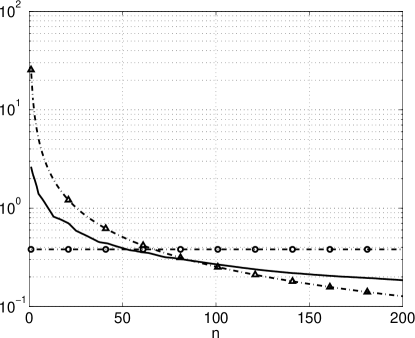
In these spaces the asymptotic behavior of the Kolmogorov width, hence of the eigenvalues, is known as recalled in Section 5. We assume here that the same bounds hold in a bounded domain (the unit disk), and we want to compare it with the discrete eigevalues of point based sets, which can be computed with one of the methods of the previous section.

To this aim, we start from a grid of equally spaced points in $[-1,1]^{2}$ restricted to the unit disk, so that the number of points inside the disk is $m\approx 10^{4}$. We use this grid both for point selection and to approximate the $L_{2}(\Omega)$ inner products as weighted pointwise products, i.e.,

$$(f,g)_{L_{2}}\approx\frac{\pi}{m}\sum_{j=1}^{m}f(x_{j})g(x_{j}).$$

We select $n=200$ points by the greedy $L_{\infty}(\Omega)$ maximization of the Power Function in the unit disk.

The eigenvalues are then computed with the method of Section 6.2, i.e, as eigenvalues of the $L_{2}(\Omega)$ Gramian of the Newton basis.

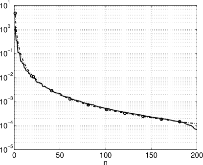
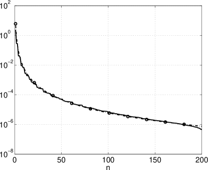
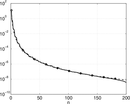
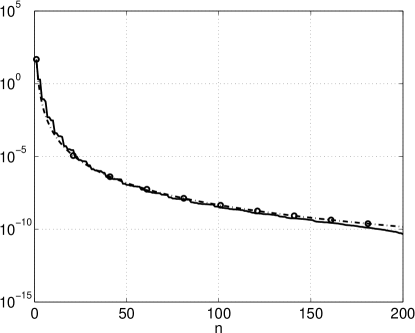
The results are shown in Figure 1. As expected, for any order under consideration there exist a positive constant $c$ such that the discrete eigenvalues decay with the same rate of the Sobolev best approximation.

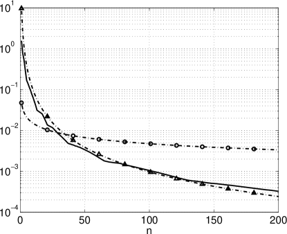
Moreover, we expect that the discrete eigenvalues converge to the true ones with a rate that can also be controlled by $\beta$. Indeed, according to Corollary 16, we have

$$0\leq\lambda_{j}-\lambda_{j,V(X_{n})}<c_{1}n^{-\beta/d},\;\;1\leq j\leq n.$$

To verify this, we instead look at the decay of

$$\sum_{j=0}^{\infty}\lambda_{j}-\sum_{j=0}^{n}\lambda_{j,V(X_{n})}.$$

since we can exactly compute the first term. Indeed, since the kernels are radial, we have

$$\sum_{j=1}^{\infty}\lambda_{j}=\int_{\Omega}K(x,x)dx=\pi K(0,0).$$

Results are presented in Figure 2. From the experiments it seems that we can improve the convergence speed somewhat, and in fact obtain a rate of order $(\beta+d/2)/d$ instead of $\beta/d$. This may be another instance of the “gap of $d/2$” already observed in [24]. Sometimes, observed convergence rates are by $d/2$ better than proven ones.

Figure 1: Decay of the discrete eigenvalues of the Matern kernels (solid line) compared with the theoretical decay rate $n^{-(\beta+d)/d}$ in the corresponding Sobolev spaces (circles). The theoretical bounds are scaled with a positive coefficient. From top left to bottom right: $\beta=0,1,2,3$.

Figure 2: Difference between the sum of the real eigenalues and the discrete ones (solid line), for the Matern kernels, compared with the theoretical decay rate $n^{-\beta/d}$ in the corresponding Sobolev spaces (circles) and with $n^{-(\beta+d/2)/d}$ (triangles). The theoretical bounds are scaled with a positive coefficient. From top left to bottom right: $\beta=0,1,2,3$.

7.2 Brownian bridge kernels

In this section we experiment with the iterated Brownian bridge kernels (see [3]). This family of kernels is useful for our purposes because the exact eigenbasis is explicitly known and the smoothness of the kernel can be controlled using a parameter.

The kernels are defined, for $\beta\in\mathbb{N}\setminus\{0\}$, $\varepsilon\geqslant 0$ and $x,y\in[0,1]$, as

$$K_{\beta,\varepsilon}(x,y)=\sum_{j=1}^{\infty}\lambda_{j}(\varepsilon,\beta)\varphi_{j}(x)\varphi_{j}(y),$$ (12)

where

$$\lambda_{j}(\varepsilon,\beta)=\left(j^{2}\pi^{2}+\varepsilon^{2}\right)^{-\beta},\quad\varphi_{j}(x)=\sin(j\pi x).$$

The kernel has $2\beta-2$ smooth derivatives.

For $\beta=1$ and $\varepsilon=0$, the kernel has the form $K_{1,0}(x,y)=\min(x,y)-xy$, but a general closed form is not known. In the following tests we will compute it using a truncation of the series (12) at a sufficiently large index. For simplicity, we will consider for now only $\varepsilon=0,1$.

Thanks to the knowledge of the explicit expansion, we can also compute the $L_{2}(\Omega)$ - Gramian of $K_{\beta,\varepsilon}$ by squaring the eigenvalues in (12), i.e.,

$$K_{\beta,\varepsilon}^{(2)}(x,y)=(K_{\beta,\varepsilon}(x,\cdot)K_{\beta,\varepsilon}(\cdot,y))_{L_{2}}=\sum_{j=1}^{\infty}\lambda_{j}(\varepsilon,2\beta)\varphi_{j}(x)\varphi_{j}(y),$$ (13)

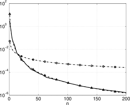
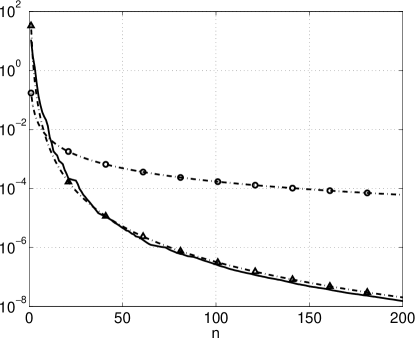
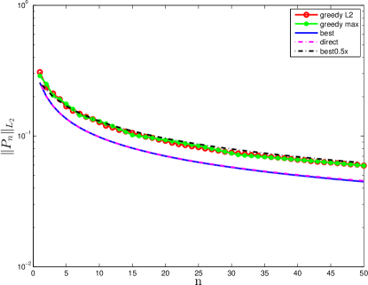
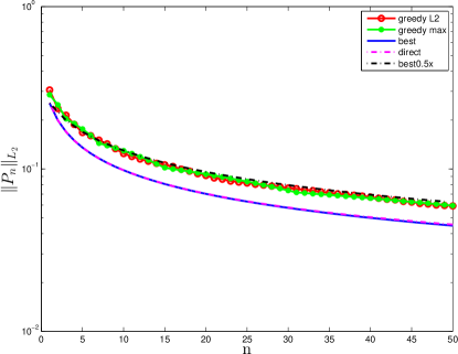
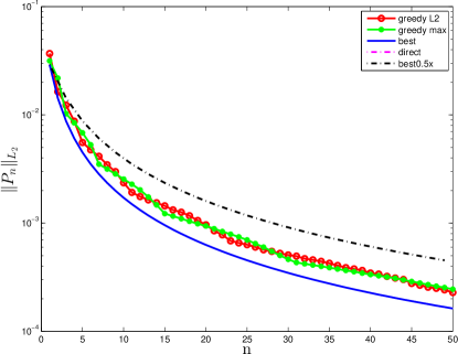
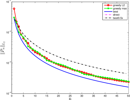
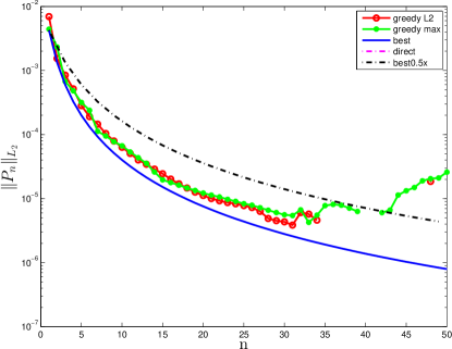
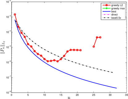
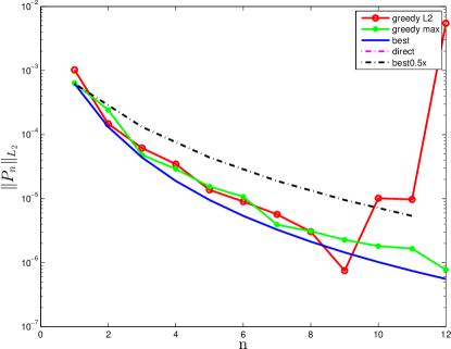
First, we want to compare the optimal decay of the power function with the one obtained by starting from a set of points $X_{N}$, both in the direct and in the greedy way. We take $N=500$ randomly distributed points in $(0,1)$ and we construct an approximation of the eigenspace $E_{n,V_{m}}$ for $n=50$.

To speed up the algorithm, for the greedy selection we approximate the $L_{2}(\Omega)$ inner product with the discrete one on $X_{N}$. This step, of course, introduces an error in the selection of the points. Nevertheless, in order to evaluate properly the performance of the algorithm, after the construction the Newton basis we compute the $L_{2}(\Omega)$ Gramian exactly, i.e., using (13).

The results for $\beta=1,\dots,4$ and $\varepsilon=0,1$ are shown in Figure 3. Lines not present in the plots mean that the corresponding power function is negative, because of numerical instability.

First, notice that the direct method is sufficiently stable only for $\beta=1$, but in this case it is able to nearly reproduce the optimal rate of decay. The greedy algorithms, on the other hand, are feasible for all the choices of the parameters, and they have a convergence between $\|P_{E_{n,m}}\|_{L_{2}}$ and $\|P_{E_{2n,m}}\|_{L_{2}}$. As the kernel becomes smoother their performance is better, but they become unstable. Observe also that the two greedy selections of the points behave essentially in the same way, even if the first one is not designed to minimize any $L_{2}(\Omega)$ norm.

Unlike for the smoothness parameter $\beta$, the dependence of the performance of the algorithm on $\varepsilon$ is not clear, except in the case $\beta=4$, where $\epsilon=1$ gives a better stability.

Figure 3: Decay of the power functions described in Section 7.2 for different parameters (from left to right: $\varepsilon=0,1$; from top to bottom: $\beta=1,2,3,4$).

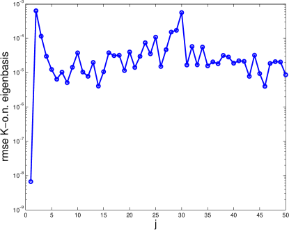
Finally, we test the convergence of the approximate eigencouples to the exact ones.

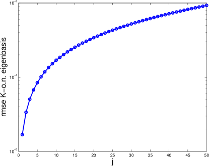
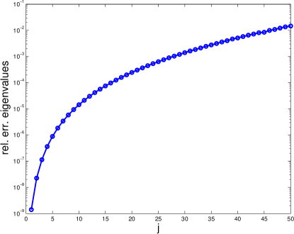
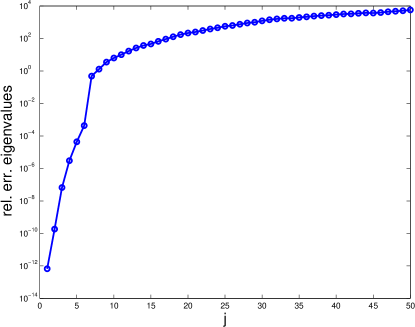
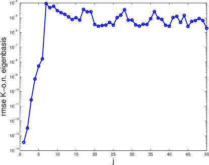
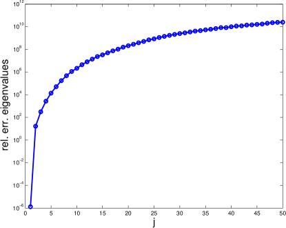
Since the method becomes unstable, we use here a smaller set of $N=100$ randomly distributed points in $(0,1)$ and we check the approximation for the first $n=50$ eigenelements. Figure 4 displays the results for $\beta=1,2,3,4$ and $\varepsilon=0$. Since the eigenbasis is defined up to a change of sign, we can expect to approximate $|\sqrt{\lambda_{j}}\varphi_{j}|$, $1\leqslant j\leqslant n$.

As expected from Proposition 13, both for the eigenvalues and the eigenfunctions the convergence is faster for smoother kernels and for the smaller indices $j$.

Also in this example the approximation becomes unstable for $\beta=4$.

Figure 4: Approximation of the eigenvalues (left) and the eigenbasis (right), for $\beta=1,2,3$ (from top to bottom), $\varepsilon=0$ and for $1\leqslant j\leqslant n$, $n=50$, as discussed in Section 7.2

References

- [1] M. Buhmann. Radial basis functions. Acta Numerica, 10:1–38, 2000.
- [2] M. Buhmann. Radial Basis Functions, Theory and Implementations. Cambridge University Press, 2003.
- [3] R. Cavoretto, G. Fasshauer, and M. McCourt. An introduction to the hilbert-schmidt svd using iterated brownian bridge kernels. Numerical Algorithms, pages 1–30, 2014.
- [4] S. De Marchi, R. Schaback, and H. Wendland. Near-optimal data-independent point locations for radial basis function interpolation. Adv. Comput. Math., 23(3):317–330, 2005.
- [5] N. Dyn, F. Narcowich, and J. Ward. Variational principles and sobolev–type estimates for generalized interpolation on a riemannian manifold. Constructive Approximation, 15(2):174–208, 1999.
- [6] G. E. Fasshauer and M. J. McCourt. Stable evaluation of Gaussian radial basis function interpolants. SIAM J. Sci. Comput., 34(2):A737–A762, 2012.
- [7] G. F. Fasshauer. Meshfree Approximation Methods with MATLAB, volume 6 of Interdisciplinary Mathematical Sciences. World Scientific Publishers, Singapore, 2007.
- [8] B. Fornberg, E. Larsson, and N. Flyer. Stable computations with Gaussian radial basis functions. SIAM J. Sci. Comput., 33(2):869–892, 2011.
- [9] B. Fornberg and C. Piret. A stable algorithm for flat radial basis functions on a sphere. SIAM J. Sci. Comput., 30:60–80, 2007.
- [10] R. Ismagilov. On n-dimensional diameters of compacts in a hilbert space. Functional Analysis and Its Applications, 2(2):125–132, 1968.
- [11] J. W. Jerome. On -widths in Sobolev spaces and applications to elliptic boundary value problems. J. Math. Anal. Appl., 29:201–215, 1970.
- [12] K. Jetter, J. Stöckler, and J. Ward. Error estimates for scattered data interpolation on spheres. Mathematics of Computation, 68:733–747, 1999.
- [13] M. A. Krasnosel′skiĭ, G. M. Vaĭnikko, P. P. Zabreĭko, Y. B. Rutitskii, and V. Y. Stetsenko. Approximate Solution of Operator Equations. Wolters-Noordhoff Publishing, Groningen, 1972. Translated from the Russian by D. Louvish.
- [14] M. Mouattamid and R. Schaback. Recursive kernels. Anal. Theory Appl., 25(4):301–316, 2009.
- [15] S. Müller and R. Schaback. A Newton basis for kernel spaces. J. Approx. Theory, 161(2):645–655, 2009.
- [16] F. J. Narcowich, R. Schaback, and J. D. Ward. Approximations in Sobolev spaces by kernel expansions. J. Approx. Theory, 114(1):70–83, 2002.
- [17] E. Novak and H. Woźniakowski. Tractability of multivariate problems. Vol. 1: Linear information, volume 6 of EMS Tracts in Mathematics. European Mathematical Society (EMS), Zürich, 2008.
- [18] M. Pazouki and R. Schaback. Bases for kernel-based spaces. Journal of Computational and Applied Mathematics, 236(4):575–588, 2011.
- [19] A. Pinkus. -Widths in Approximation Theory, volume 7 of Ergebnisse der Mathematik und ihrer Grenzgebiete (3) [Results in Mathematics and Related Areas (3)]. Springer-Verlag, Berlin, 1985.
- [20] W. Pogorzelski. Integral Equations and Their Applications. Vol. I. Translated from the Polish by Jacques J. Schorr-Con, A. Kacner and Z. Olesiak. International Series of Monographs in Pure and Applied Mathematics, Vol. 88. Pergamon Press, Oxford, 1966.
- [21] R. Schaback. Error estimates and condition numbers for radial basis function interpolation. Adv. Comput. Math., 3(3):251–264, 1995.
- [22] R. Schaback. Native Hilbert spaces for radial basis functions I. In M. Buhmann, D. H. Mache, M. Felten, and M. Müller, editors, New Developments in Approximation Theory, number 132 in International Series of Numerical Mathematics, pages 255–282. Birkhäuser Verlag, 1999.
- [23] R. Schaback and H. Wendland. Approximation by positive definite kernels. In M. Buhmann and D. Mache, editors, Advanced Problems in Constructive Approximation, volume 142 of International Series in Numerical Mathematics, pages 203–221, 2002.
- [24] R. Schaback and H. Wendland. Inverse and saturation theorems for radial basis function interpolation. Math. Comp., 71(238):669–681 (electronic), 2002.
- [25] R. Schaback and H. Wendland. Kernel techniques: from machine learning to meshless methods. Acta Numerica, 15:543–639, 2006.
- [26] H. Sun and Q. Wu. Application of integral operator for regularized least-square regression. Math. Comput. Modelling, 49(1-2):276–285, 2009.
- [27] H. Wendland. Scattered Data Approximation, volume 17 of Cambridge Monographs on Applied and Computational Mathematics. Cambridge University Press, Cambridge, 2005.