Towards a new determination of the QCD Lambda parameter from running couplings in the three-flavour theory

Abstract:

We review our new strategy and current status towards a high precision computation of the Lambda parameter from three-flavour simulations in QCD. To reach this goal we combine specific advantages of the Schrödinger functional and gradient flow couplings.

1 Introduction

In our understanding of the Standard Model the strong coupling $\overline{g}(\mu)$ plays an essential rôle as its parametric uncertainty is one of the dominant sources of uncertainty in Higgs decays for instance. Using lattice gauge theory we are in the fortunate position to study QCD for any number of dynamical flavours $N_{\rm f}$. In contrast to any experimental data analysis in high energy physics, we are able to employ non-perturbative definitions of the strong coupling by means of any suitable lattice observable $O_{\rm lat}$, such that [1]

$$\overline{g}^{2}(\mu) =\lim_{a\to 0}{\rm c}_{O}(a,\mu)\cdot O_{\rm lat}(a,\mu)\;.$$ (1)

The normalization factor ${\rm c}_{O}(a,\mu)$ guarantees $\overline{g}^{2}=g_{0}^{2}+{\rm O}(g_{0}^{4})$ at leading order in lattice perturbation theory. Any lattice observable fulfilling eq. (1) defines a renormalization scheme with a different scale-dependent renormalized coupling. As in QCD conformal symmetry of the massless Lagrangian is broken on the quantum level, one can define a renormalization group (RG) invariant, the $\Lambda$-parameter,

$$\Lambda \equiv\mu\big{[}{b_{0}\overline{g}^{2}(\mu)}\big{]}^{-{b_{1}}/({2b_{0}^{2}})}\,{\rm e}^{-1/({2b_{0}\overline{g}^{2}(\mu)})}\exp\bigg{\{}\!\!-\!\!\int_{0}^{\overline{g}^{\vphantom{A}}(\mu)}\!{\rm d}g\bigg{[}\dfrac{1}{\beta(g)}+\dfrac{1}{b_{0}g^{3}}-\dfrac{b_{1}}{b_{0}^{2}g}\bigg{]}\bigg{\}}\;.$$ (2)

This definition holds for any $\mu$, and its value is trivially scheme-dependent in the sense that the ratio $\Lambda_{1}/\Lambda_{2}$ for two different schemes can be computed exactly. It has become standard to quote $\overline{g}^{2}$ at the electroweak scale given by the $Z$-boson mass, $\mu=M_{Z}$, in the intrinsically perturbative $\overline{\rm MS}$ scheme.

A fully non-perturbative computation of the $\Lambda$-parameter through lattice computations proceeds in the following way. One chooses an appropriate definition of a renormalized coupling (1) in a finite-volume renormalization scheme which interlinks the energy scale and the finite size of the system, $\mu\propto L^{-1}$. Starting at a high energy scale where perturbation theory is applicable without doubt, say at $\mu_{\rm PT}\sim M_{Z}\sim 100\;{\rm GeV}$, one iteratively applies a finite-size rescaling technique by computing the change of the renormalized coupling from a change of energy scales (or $L$) by factors of $s=2$ for instance. After $N$ steps one arrives at some hadronic scale $\mu_{\rm had}=\mu_{\rm PT}/s^{N}\equiv L_{\rm max}^{-1}$, where a connection to large volume (LV) lattice simulations can be established. This allows to determine $\Lambda$ in terms of some experimentally known hadronic observable, $f_{\rm had}$, used to set the overall energy scale in the LV simulations, and thus in physical units. For $\Lambda_{\overline{\rm MS}}$ this strategy decomposes as follows:

$$\Lambda_{\overline{\rm MS}} =\left[f_{\rm had}\right]_{\rm exp}\times\left[\frac{\Lambda_{\overline{\rm MS}}}{\Lambda}\right]_{\rm exact}\times\frac{\Lambda}{f_{\rm had}} \frac{\Lambda}{f_{\rm had}} =\frac{L_{\rm max}\Lambda}{L_{\rm max}f_{\rm had}}\;.$$ with (3)

The total error on $\Lambda$ is composed of that from the LV scale setting $(L_{\rm max}f_{\rm had})$ and the determination of $L_{\rm max}\Lambda$ from the non-perturbative running in the intermediate, finite-volume scheme. While for $N_{\rm f}=2$ [2] the error of $L_{\rm max}f_{\rm had}\equiv L_{1}f_{\rm K}=0.315(8)(2)$ contributed about $\tfrac{2}{5}$ to the total error of 6% on ${\Lambda}/{f_{\rm had}}$, it will become negligible in the near future due to new developments [3]. The current world average(s) for $\alpha^{(5)}_{\rm s}(M_{Z})$ are $0.1183(12)$ from PDG [4] using experiments only, and $0.1184(12)$ from the average of present lattice determinations [1]. This 1% error translates into an error of about 6% in $\Lambda_{\overline{\rm MS}}^{(5)}$. For our new estimate of $\Lambda^{(N_{\rm f}=3)}/f_{\rm had}$, to be derived from LV lattices within the current CLS effort [5], it is thus worthwhile to aim for an accuracy of about 4% or better.

2 Why choose a new strategy?

We have seen that by mainly controlling the accuracy of the non-perturbative RG running, we can improve the determination of $\Lambda$. In the past, the Schrödinger functional (SF) coupling $\overline{g}_{\rm SF}$ [6] has been the most useful definition of a finite-volume renormalization scheme compatible with the strategy behind eq. (3). A more recent development that can be used along the same lines, is given by one of the many running coupling definitions employing the Yang–Mills gradient flow (GF) [7], $\overline{g}_{\rm GF}$ in short. Initially introduced in [8] it has been studied in a finite-volume setup in [9, 10, 11]. Especially, the apparently much better noise-to-signal ratio of $\overline{g}_{\rm GF}$ raises hope to significantly increase the accuracy in the RG running. To what extent this statement complies with the renormalization group running covering two orders of magnitude in energy scales, we will see below. First we start with a general comparison of SF and GF couplings, both defined with Dirichlet boundary conditions in time. A short summary is given in table 1.

topic	SF coupling	GF coupling	remark
Definition	$\overline{g}^{2}_{\rm SF}(L)=k\langle\tfrac{\partial\Gamma}{\partial\eta}\rangle^{-1}_{\eta=0}$	$\overline{g}^{2}_{\rm GF}(L)=\langle t^{2}E\rangle/\mathcal{N}$
SF boundary field	$\neq 0$	$=0$
PT matching $\sim$ 64 GeV	2-loop	tree-level	GF @ higher energies
typical # meas.	O(100 000)	O(1000)	$\Delta\overline{g}^{2}_{\tiny\rm SF}\!\simeq\!\Delta\overline{g}^{2}_{\rm GF}$
($\tau_{\rm int}$, $\mathcal{V}$, …)			$L\approx\!0.4\,{\rm fm}$
cutoff effects	mild	rather large (so far)
	2-loop improvement	tree-level improvement
	$\Rightarrow{L}/{a}=6\ldots 12$	$\Rightarrow{L}/{a}=8\ldots 16$	controlled $a\to 0$
$\Delta\overline{g}^{2}/\overline{g}^{2}$	$\sim\overline{g}^{2}$	const.	for fixed #meas.
$\Rightarrow\Delta L/L$	const.	$\sim\text{const}/\overline{g}^{2}$

Table 1: General comparison of gradient flow and SF running coupling schemes.

The SF coupling, $\overline{g}_{\rm SF}(L)$, is defined as the response to a variation of the (QCD) action about a non-vanishing Yang–Mills background field imposed through boundary conditions at Euclidean time $x_{0}=0,T$ $(T=L)$ [12]. As such it is entirely sensitive to the physical extent $L$. The coupling $\overline{g}_{\rm GF}(L)$ on the other hand is also sensitive to short distances since it is given by the Yang–Mills energy density defined with vanishing background field at finite gradient flow time $t=(cL)^{2}/8$ for some fixed constant $c\in[0.25,0.5]$ [10]. While for both definitions the tree-level normalization ${\rm c}_{O}(a,\mu)$ is known for different lattice actions [12, 10, 11], cutoff effects are mild for $\overline{g}_{\rm SF}$ but large for $\overline{g}_{\rm GF}$. Additionally, for the SF coupling perturbative improvement is known up to 2-loop order but unknown for the GF coupling. Both facts together with additional details such as the respective integrated autocorrelation time, statistical variance and so on, influence the precision of the continuum limit of the lattice step-scaling function $\Sigma$,

$$\sigma(u) =\lim_{a\to 0}\Sigma(u,a/L)\;, \Sigma(u,a/L) =\left.\overline{g}^{2}(2L)\right|_{\overline{g}^{2}(L)=u,Lm=0}\;.$$ (4)

It has to be computed numerically at chosen values of $u_{n}\equiv\overline{g}^{2}(L_{n})$, $n\in\{1,\ldots,N\}$ in order to cover the energy range under consideration. From past experience we expect that lattice sizes $L/a<12$ are sufficient to control the continuum extrapolation of $\Sigma_{\rm SF}(u,a/L)$. On the other hand lattices with $L/a>8$ are needed to achieve an equivalent accuracy in the computation of $\Sigma_{\rm GF}(u,a/L)$. At a fixed volume with $L\approx 0.4\,{\rm fm}$, and choosing $c\equiv\sqrt{8t}/L=0.3$ such that $\overline{g}_{\rm SF}^{2}(L)\simeq\overline{g}_{\rm GF}^{2}(L)$, a numerical study has shown that in order to achieve the same accuracy in both couplings one needs 100 times more measurements of $\overline{g}_{\rm SF}^{2}$.

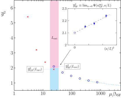
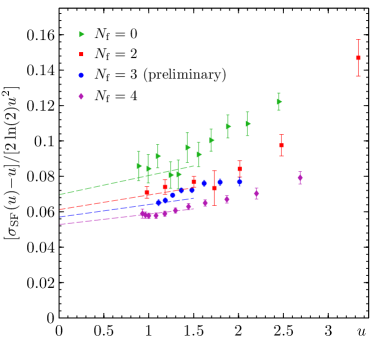
Figure 1: (Left) Sketch of our proposed strategy to non-perturbatively switch running coupling schemes at an intermediate energy scale $\mu_{\rm swi}=1/L_{\rm swi}$. (Right) Data of SF step-scaling functions for different dynamical flavour content, $N_{\rm f}=0,2,3,4$ [12, 14, 15], and its leading asymptotic form $b_{0}+{\rm O}(u)$ (dashed lines).

Finally, the two couplings show a very different leading scaling behaviour of the relative error $R_{\overline{g}^{2}}\equiv\Delta\overline{g}^{2}/\overline{g}^{2}$ which directly translates via the RG into $R_{L}\equiv\Delta L/L=-\Delta\overline{g}^{2}\big{/}2\overline{g}\beta(\overline{g})$. Considering only the dominant contribution, $\beta(\overline{g})\simeq-b_{0}\overline{g}^{3}$, this results into an error of $R_{L}=R_{\overline{g}^{2}}\big{/}2b_{0}\overline{g}^{2}$, with $(2b_{0})^{-1}\approx 9$ in three-flavour QCD. With a behaviour of $R_{\overline{g}^{2}_{\rm SF}}\sim\overline{g}^{2}$ and $R_{\overline{g}^{2}_{\rm GF}}\sim\text{const}$, a relative scale uncertainty of $\Delta L/L\sim\text{const}$ follows for the SF coupling and $\Delta L/L\sim 1/\overline{g}^{2}$ for GF couplings at a fixed number of independent measurements.

Every step in the finite-size scaling method contributes to the total error budget of the RG running, giving as first rough estimate

$$\left(\frac{\Delta[L_{\rm max}\Lambda]}{L_{\rm max}\Lambda}\right)^{2} \simeq\sum_{n=1}^{N}\left(\frac{\Delta L}{L}\Big{|}_{u_{n}}\right)^{2}\;, u_{n} =\sigma^{-1}(u_{n-1})\;, u_{0} =\overline{g}^{2}(L_{\rm max})\;.$$ (5)

From this point of view it should be clear that at constant effort, the SF coupling accumulates approximately the same error in each step while the GF coupling definition shows an error that is steadily growing towards the high energy regime. Of course, if computational costs are irrelevant this problem could be solved by brute force calculations. So far we have discussed both schemes under the aspect of statistical accuracy only, but there are more points to be taken into account, for instance the matching to PT at high energies. For $\overline{g}_{\rm SF}$ the matching coefficients in $\overline{g}^{2}_{s}=\overline{g}^{2}_{s^{\prime}}+\sum^{\ell}_{k=1}\chi^{(k)}\overline{g}^{2k+2}_{s^{\prime}}$ are known up to $\ell=2$ loop order [17] while no coefficient is known for $\overline{g}_{\rm GF}$ so far. Even with a given 1-loop coefficient, $\overline{g}_{\rm GF}$ still has to be matched at higher energies to control this step equally well, and thus increases the costs and statistical error in the RG running. Additional points will be elucidated in more detail in a forthcoming publication.

Having the global aspect of our strategy in mind we have to conclude that the GF coupling scheme is advantageous at hadronic scales while the SF coupling scheme still is to be favoured at high energy scales.

3 Changing the standard strategy

From the facts presented in the previous section the optimised way to improve the computation of $\Lambda$ seems to be to combine both schemes. As depicted in the left panel of Fig. 1, one computes the running of the chosen gradient flow coupling at low energies up to an energy scale of $\mu_{\rm swi}=1/L_{\rm swi}\equiv s^{K}/L_{\rm max}$:

$$u^{\rm GF}_{k} =\overline{g}_{\rm GF}^{2}(L_{\rm max}/s^{k})\;,\quad k\in\{0,1,\ldots,K\}\;, u^{\rm GF}_{0} =\overline{g}_{\rm GF}^{2}(L_{\rm max})\;,$$

$$\sigma_{\rm GF}\left(\overline{g}_{\rm GF}^{2}(L/s)\right) =\overline{g}_{\rm GF}^{2}(L)\;, u^{\rm GF}_{\rm swi} =\overline{g}_{\rm GF}^{2}(L_{\rm max}/s^{K})\;.$$ (6)

At the scheme-switching scale $L_{\rm swi}$ one has to set up additional simulations defined through a line of constant physics, $(\overline{g}_{\rm GF}^{2}(L_{\rm swi}),L_{\rm swi}m)=(u^{\rm GF}_{\rm swi},0)$, in order to compute the SF coupling via

$$u^{\rm SF}_{\rm swi} =\lim_{a\to 0}\Psi(u,a/L)\;, \Psi(u,a/L) =\left.\overline{g}_{\rm SF}^{2}(L)\right|_{u=u^{\rm GF}_{\rm swi},L_{\rm swi}m=0}\;,$$ (7)

as accurately as possible. From here on one continues in the new scheme

$$u^{\rm SF}_{m} =\overline{g}_{\rm SF}^{2}(L_{\rm swi}/s^{m})\;,\quad m\in\{0,1,\ldots,M\}\;, u^{\rm SF}_{0} =\overline{g}_{\rm SF}^{2}(L_{\rm swi})\;,$$

$$\sigma_{\rm SF}\left(\overline{g}_{\rm SF}^{2}(L/s)\right) =\overline{g}_{\rm SF}^{2}(L)\;, u^{\rm SF}_{\rm PT} =\overline{g}_{\rm SF}^{2}(L_{\rm swi}/s^{M})\;,$$ (8)

with $M=N-K$ if the same scale difference is to be covered as originally anticipated by $\mu_{\rm PT}^{-1}=L_{\rm max}/s^{N}$, and where ultimately the connection to the perturbative running can be safely established. We remark that we could have started our discussion also at high energies, i.e., reversing the strategy and interchanging SF and GF in eq. (7). In fact, carrying out both procedures might help to increase control over this non-perturbative scheme-switching step.

4 Present status

For various practical reasons we have started with the running of the SF coupling from high to intermediate energies, reaching couplings as large as $u^{\rm SF}=2$ within our new strategy. We are working in a massless renormalization scheme with $N_{\rm f}=3$ quark flavours and thus need to tune to vanishing PCAC quark mass, $Lm=0$, for plaquette gauge action and non-perturbatively ${\rm O}(a)$ improved Wilson quarks. This has been done for lattice sizes $L/a=4,\dots,16$ and bare gauge couplings $6\leq\beta\equiv 6/g_{0}^{2}\leq 9$. To minimise tuning efforts in subsequent projects, we have done this more precisely than in the past, allowing us to smoothly parameterise the critical line $m_{\rm crit}(g_{0}^{2},a/L)$ on the considered lattice sizes for $0\leq g_{0}^{2}\leq 1$. Employing the perturbative 2-loop formula for $m_{\rm crit}(g_{0}^{2},a/L)$, we use the fit ansatz

$$am_{\rm crit}(g_{0}^{2},a/L) =[am_{\rm crit}(g_{0}^{2},a/L)]_{\text{2-lp}}+k_{1}(a/L)\cdot g_{0}^{6}+k_{2}(a/L)\cdot g_{0}^{8}+k_{3}(a/L)\cdot g_{0}^{10}$$ (9)

to describe our data, c.f. left panel of Fig. 2. The difference between a direct fit for each $L/a$ and global fits with varying coefficient functions $k_{1},k_{2},k_{3}$ serves as a quality criteria for our interpolating function. We know that for the accuracy we are aiming at, any additional uncertainty from a tuning to a line of constant physics becomes negligible, if $|Lm|<0.005$ is satisfied. Our final estimates fulfill $|Lm|<0.001$.

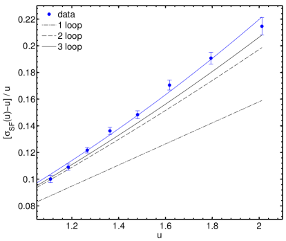
Figure 2: (Left) Data and interpolating functions for critical line $m_{\rm crit}(g_{0}^{2},a/L)$ along constant $L/a$. (Right) Non-perturbative continuum step-scaling function $\sigma_{\rm SF}(u)$ vs. perturbative evaluation.

To compute the SF step-scaling function $\sigma_{\rm SF}(u)$ we aim for simulations with $1.1\leq u^{\rm SF}\leq 2$, uniformly distributed in $1/u^{\rm SF}$. For $L/a\in\{4,6,8\}$ we use 8 different $\beta$ values but simulate only three for $L/a\in\{10,12\}$ in order to minimise computational costs in the finite-size rescaling step $L\to 2L$. Along the lines of [16, 15] we interpolate our data for $\overline{g}_{\rm SF}^{2}(\beta,L/a)$ and $\overline{g}_{\rm SF}^{2}(\beta,2L/a)$. The computation of the two-loop improved lattice step-scaling function $\Sigma_{\rm SF}^{(2)}(u^{\rm SF},a/L)$ [17] thus requires $\overline{g}_{\rm SF}^{2}(\beta,L/a)$ to be fixed at certain values of $u^{\rm SF}$ in line with (8). The continuum limit is taken individually at each value of $u^{\rm SF}_{m}$ with full error propagation. The coarsest lattice only serves the purpose of estimating the size of cutoff effects but is never taken into account in the analysis. Furthermore, data for $2L/a=20$ is still missing and cannot be included at present. The plot provided in Fig. 3 thus shows a (preliminary) continuum limit of $\Sigma_{\rm SF}^{(2)}(u,a/L)$ using a local fit ansatz with linear scaling in $(a/L)^{2}$ towards the continuum. This gives the largest error on $\sigma_{\rm SF}(u)$ which will be improved after studying appropriate global fit ansätze in more detail. With the data at hand we use the standard interpolation

$$\sigma(u) =u+s_{0}u^{2}+s_{1}u^{3}+s_{2}^{\rm fit}u^{4}+s_{3}^{\rm fit}u^{5}\;, s_{0} =2\ln(2)b_{0}\;, s_{1} =s_{0}^{2}+2\ln(2)b_{1}\;,$$ (10)

with parameters $s_{2}^{\rm fit},s_{3}^{\rm fit}$ and $s_{0}$, $s_{1}$ taken from perturbation theory. In Fig. 2 we plot the data points and interpolating fit function of $\sigma_{\rm SF}(u)$ together with their known perturbative behaviour and remark that the important information lies in the well-defined error of the former. To look at our current results from a global perspective, we compare it in Fig. 1 (right panel) to previous determinations of $\sigma_{\rm SF}$ for $N_{\rm f}=0,2,4$. For a better discrimination we plot $[\sigma_{\rm SF}(u)-u]/[2\ln(2)u^{2}]$ such that the axis intercept corresponds to $b_{0}$. This figure provides a beautiful demonstration of our current understanding of asymptotic freedom at the non-perturbative level.

5 Conclusions & Outlook

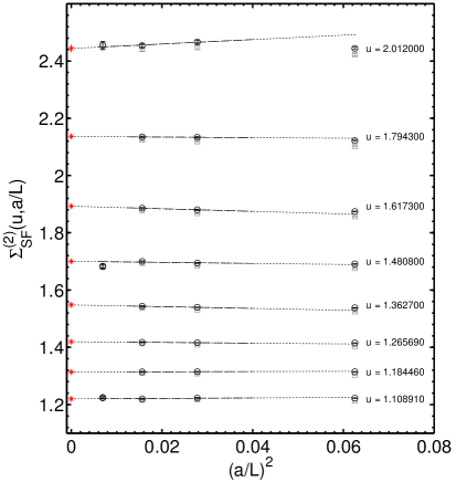
Figure 3: Local (preliminary) continuum extrapolations of $\Sigma_{\rm SF}^{(2)}(u^{\rm SF},a/L)$ using $L/a\geq 6$ lattices.

We have presented an extension to the ALPHA-strategy towards future high precision computations of the Lambda parameter. It still keeps all systematic errors under control by following a traditional finite-size scaling approach to non-perturbatively connect low- and high-energy regimes. The gain in precision is achieved by exploiting complementary properties of the SF and gradient flow coupling together with a non-perturbative scheme switch at intermediate energies. While the SF part of the computations has been finished we are now working on the computation of the gradient flow step-scaling function and the non-perturbative scheme-switching step.

References

- [1] S. Aoki et al., Eur.Phys.J. C74 (2014) 2890, 1310.8555.
- [2] ALPHA, P. Fritzsch et al., Nucl.Phys. B865 (2012) 397, 1205.5380.
- [3] M. Dalla Brida and S. Sint, PoS LATTICE2014 (2014) 280.
- [4] Particle Data Group, J. Beringer et al., Phys.Rev. D86 (2012) 010001, and 2013 partial update for the 2014 edition.
- [5] M. Bruno et al., (2014), 1411.3982.
- [6] M. Lüscher et al., Nucl.Phys. B384 (1992) 168, hep-lat/9207009.
- [7] R. Narayanan and H. Neuberger, JHEP 0603 (2006) 064, hep-th/0601210.
- [8] M. Lüscher, JHEP 1008 (2010) 071, 1006.4518.
- [9] Z. Fodor et al., JHEP 1211 (2012) 007, 1208.1051.
- [10] P. Fritzsch and A. Ramos, JHEP 1310 (2013) 008, 1301.4388.
- [11] A. Ramos, (2014), 1409.1445.
- [12] M. Lüscher et al., Nucl.Phys. B413 (1994) 481, hep-lat/9309005.
- [13] A. Ramos and S. Sint, PoS LATTICE2014 (2014) 329.
- [14] ALPHA, M. Della Morte et al., Nucl.Phys. B713 (2005) 378, hep-lat/0411025.
- [15] ALPHA, F. Tekin, R. Sommer and U. Wolff, Nucl.Phys. B840 (2010) 114, 1006.0672.
- [16] T. Appelquist, G. Fleming and E. Neil, Phys. Rev. D 79 (2009).
- [17] ALPHA, A. Bode, P. Weisz and U. Wolff, Nucl.Phys. B576 (2000) 517, hep-lat/9911018, [Erratum-ibid. B 600 (2001) 453], [Erratum-ibid. B 608 (2001) 481].