Electron-phonon interaction in a spin-orbit coupled quantum wire with a gap

Abstract

Interaction between electron and acoustic phonon in an in-plane magnetic field induced gapped quantum wire with Rashba spin-orbit interaction is studied. We calculate acoustic phonon limited resistivity ($\rho$) and phonon-drag thermopower ($S_{g}$) due to two well known mechanisms of electron-phonon interaction namely, deformation potential (DP) and piezoelectric (PE) scattering. In the so called Bloch-Gruneisen temperature limit both $\rho$ and $S_{g}$ depend on temperature ($T$) in a power law fashion i.e. $\rho$ or $S_{g}\sim T^{\nu_{T}}$. For resistivity, $\nu_{T}$ takes the value $5$ and $3$ due to DP and PE scattering respectively. On the other hand, $\nu_{T}$ is $4$ and $2$ due to DP and PE scattering, respectively for phonon-drag thermopower. Additionally, we find numerically that $\nu_{T}$ depends on Rashba parameter ($\alpha$) and electron density ($n$). The dependence of $\nu_{T}$ on $\alpha$ becomes more prominent at lower density. We also study the variations of $\rho$ and $S_{g}$ with carrier density in the Bloch-Gruneisen regime. Through a numerical analysis a similar power law dependence $\rho$ or $S_{g}\sim n^{-\nu_{n}}$ is established in which the effective exponent $\nu_{n}$ undergoes a smooth transition from a low density behavior to a high density behavior. At a higher density regime, $\nu_{n}$ matches excellently with the value obtained from theoretical arguments. Approximate analytical expressions for both resistivity and phonon-drag thermopower in the Bloch-Gruneisen regime are given.

I Introduction

Due to the promising applications in the area of quantum information processinginform and device technology,device spin dependent phenomenaspin1 ; spin2 ; spin3 in low dimensional structures have been of major interest in scientific communities for several years. The main route of spin related phenomena is the well known spin-orbit interaction (SOI). In semiconductor structures, SOI originates due to the inversion symmetry breaking either in the bulk or at the hetero-interface. Band bending in heterostructure gives rise to an electric field to produce an asymmetric confining potential which itself is responsible for generating a SOI of Rashba type.rashba The strength of Rashba SOI is proportional to the magnitude of the electric field generated and hence is tunabletune1 ; tune2 with the aid of an external gate voltage. Another kind of SOI, usually termed as Dresselhaus SOI,Dressh originates due to the breaking of inversion symmetry in the bulk crystal. In general the strengthstrng_RD of the Dresselhaus SOI is smaller than that of Rashba SOI in heterostructure. The case of equal strength of both SOIs is of particular importance for future scope of developing non-ballistic spin field effect transistor.NBspin_FET

In a quantum well, restriction of carrier’s motion by an additional confinement in a particular direction essentially leads to the formation of a quantum wire (QW). The width of QW is of the order of the Fermi wave length in order to allow ballistic transport.BLT_QW Semiconductor QW with SOI is considered as a building block for a better implementationspinFT of spin-field effect transistor.Datta_Das An in-plane magnetic field along the wire direction lifts the $k=0$ degeneracy in a spin-orbit coupled QW and as a result a gap is induced in the energy spectrum. Immense interests have been grown on the gapped spin-orbit coupled QW because of several proposals of asymmetric spin filtering,helix1 controlling impuritiesmag_imp by a magnetic field, topological superconducting phase,topo_ph1 ; topo_ph2 ; topo_ph3 helical stateshelix1 ; topo_ph2 ; helix2 ; helix3 etc. Recently, magnetic field induced spin-orbit gap in an one dimensional hole gas has been realized experimentally.helix3

In the present study we mainly focus on various consequences of electron-phonon interaction in a spin-orbit coupled gapped QW by calculating phonon limited resistivity and phonon-drag thermopower in the Bloch-Gruneisen (BG) regime. In the BG regime, the resistivity differs abruptly from its equipartition behavior. An upper bound of the BG regime can be defined by the characteristic temperature $T_{BG}=2\hbar v_{s}k_{F}/k_{B}$, where $v_{s}$ is the sound velocity and $k_{F}$ is the Fermi wave vector. Below $T_{BG}$ the acoustic phonon energy is comparable with the thermal energy. Due to the smallness of Fermi surface in semiconductor structures, acoustic phonon with wave vector $q\simeq 2k_{F}$ can not be excited appreciably which in turn leads to a complicated temperature dependence of resistivity below $T_{BG}$. The existence of the BG regime in semiconductor quantum well has been confirmed experimentally.BG_obs Another important quantity that can be used to probe the electron-phonon interaction in semiconductor nanostructure is the phonon-drag contribution to the thermoelectric power. A number studies have been performed to understand the behavior of phonon limited mobilityph_mob1 ; ph_mob2 ; ph_mob3 ; ph_mob1d1 ; ph_mob1d2 ; ph_mob1d3 ; ph_mob1d4 ; ph_mob1d5 and phonon-drag thermopowerphdrg1 ; phdrg2 ; phdrg3 ; phdrg4 ; phdrg5 in quantum well and wire for several years. Recently, acoustic phonon limited resistivitytutul1 and phonon-drag thermopowertutul2 in a Rashba spin-orbit coupled two dimensional electron gas have been studied. It is revealed through a numerical analysis that the effective exponents of the temperature dependence of both resistivity and thermopower depend significantly on the strength of the Rashba SOI.

In BG regime, we find analytically that both resistivity and phonon-drag thermopower in a spin-orbit coupled gapped QW maintains a power law dependence with temperature i.e. $\rho$ or $S_{g}\sim T^{\nu_{T}}$. The effective exponent $\nu_{T}$ is $5$ and $3$ due to deformation potential (DP) and piezoelectric (PE) scattering, respectively in the case of phonon limited resistivity. For phonon-drag thermopower $\nu_{T}$ becomes $4$ and $2$ due to DP and PE scattering, respectively. The exponent $\nu_{T}$ has also been extracted numerically which clearly undergoes a transition from BG regime to equipartition limit. At a relatively higher density, $\nu_{T}$ is in excellent agreement with the analytical results. Temperature variation of $\nu_{T}$ for different Rashba parameter ($\alpha$) at a fixed density has also been shown. The effect of $\alpha$ on the temperature dependence of $\nu_{T}$ becomes less prominent as one approaches towards higher density. Additionally, the dependence of both $\rho$ and $S_{g}$ on carrier density has been shown in which both quantities undergo a transition from a relatively low to a higher density behavior.

We organize this paper in the following way. In section II we present all the theoretical details. Numerical results and discussions have been reported in section III. We summarize our work in section IV.

II Theory

II.1 Physical system

We consider a semiconductor QW of radius $R$ in which electrons are free to move in the $z$- direction. Rashba SOI in a QW essentially breaks the spin-degeneracyzulicke by shifting the non-degenerate subbands laterally along the wave vector. But the spectrum is still degenerate at $k=0$. An external magnetic field ${\bf B}=B\hat{z}$ along the wire direction can be used to lift this degeneracy further by inducing a gap $\Delta$ in the energy spectrum.helix1 ; privman ; meden Now the single particle Hamiltonian describing a gapped QW with Rashba SOI is written as

$$H=\Big{(}\frac{p^{2}}{2m^{\ast}}+V({\bf r})\Big{)}\sigma_{0}+\frac{\alpha}{\hbar}\sigma_{y}p+\Delta\sigma_{z},$$ (1)

where $p=\hbar k$ is the electron momentum in the $z$- direction, $m^{\ast}$ is effective mass of electron, $\sigma_{0}$ is the unit matrix, $\sigma_{i}$’s are the Pauli spin matrices, and $\alpha$ is the strength of RSOI. Also $\Delta=g^{\ast}\mu_{B}B/2$ is the Zeeman energy with $g^{\ast}$ and $\mu_{B}$ as the effective Lande $g$- factor and Bohr magneton, respectively. Finally, $V({\bf r})$ is the confining potential in the transverse direction ${\bf r}\equiv(x,y)$.

The wire is assumed to be thin enough so that only the lowest subband in the transverse direction is occupied by electrons. By diagonalizing Eq. (1), the eigen energies corresponding to the present physical system can be found in the following form

$$\epsilon_{k}^{\lambda}=\frac{\hbar^{2}k^{2}}{2m^{\ast}}+\lambda\sqrt{\alpha^{2}k^{2}+\Delta^{2}},$$ (2)

where $\lambda=\pm$ describes the branch index. Note that the energy is measured from the bottom of the lowest sub-band energy $\varepsilon_{10}=\hbar^{2}k_{10}^{2}/(2m^{\ast})$ with $k_{10}$ as the sub-band wave vector.

The eigen functions corresponding to the $+$ and $-$ branches are respectively given by

$$\Psi^{+}(r,z)=\frac{e^{ikz}}{\sqrt{2\pi}}\begin{pmatrix}\cos{\frac{\phi_{k}}{2}}\\ i\sin{\frac{\phi_{k}}{2}}\end{pmatrix}\Phi_{10}(r),$$ (3)

and

$$\Psi^{-}(r,z)=\frac{e^{ikz}}{\sqrt{2\pi}}\begin{pmatrix}\sin{\frac{\phi_{k}}{2}}\\ -i\cos{\frac{\phi_{k}}{2}}\end{pmatrix}\Phi_{10}(r),$$ (4)

where $\tan{\phi_{k}}=\alpha k/\Delta$. The lowest subband wave function for $r\leq R$ is given by $\Phi_{10}(r)=J_{0}(k_{10}r)/\{\sqrt{\pi R^{2}}J_{1}(k_{10}R)\}$ with $J_{\nu}(x)$ as the Bessel function of order $\nu$. It is important to mention that $k_{10}R$ is the first zero of $J_{0}(k_{10}R)$. Out side the quantum wire $\Phi_{10}(r)$ vanishes.

At a fixed energy namely, Fermi energy $\epsilon_{F}$, one can have the following expression for the Fermi wave vectors

$$k_{F}^{\lambda}=\Bigg{\{}\bigg{(}-\lambda k_{\alpha}+\sqrt{k_{\alpha}^{2}+\frac{2m^{\ast}\epsilon_{F}}{\hbar^{2}}+\frac{\Delta^{2}}{\alpha^{2}}}\bigg{)}^{2}-\frac{\Delta^{2}}{\alpha^{2}}\Bigg{\}}^{\frac{1}{2}},$$ (5)

where $k_{\alpha}=m^{\ast}\alpha/\hbar^{2}$. In the $B\rightarrow 0$ limit, Eq. (5) reduces to the known forms of the Fermi wave vectors of a Rashba spin-orbit coupled quantum wire.

The velocity corresponding to the energy spectrum given in Eq. (2) is calculated as

$$v_{k}^{\lambda}=\frac{\hbar k}{m^{\ast}}+\lambda\frac{\alpha^{2}k}{\hbar\sqrt{\alpha^{2}k^{2}+\Delta^{2}}}.$$ (6)

II.2 Phonon limited resistivity

In this section we shall calculate resistivity due to the electron-phonon interaction using Boltzmann transport theory. We restrict ourselves to consider only the longitudinal and transverse acoustic phonon modes. Using Drude’s formula, the resistivity is simply written as

$$\rho=\frac{m^{\ast}}{ne^{2}}\Big{\langle}\frac{1}{\tau}\Big{\rangle},$$ (7)

where $\langle 1/\tau\rangle$ is the inverse relaxation time (IRT) averaged over energy and $n$ is the density of electron.

The energy averaged IRT for a specific energy branch $\lambda$ is given by

$$\Big{\langle}\frac{1}{\tau^{\lambda}}\Big{\rangle}=\frac{2}{k_{B}T}\int d\epsilon_{k}^{\lambda}f(\epsilon_{k}^{\lambda})\{1-f(\epsilon_{k}^{\lambda})\}\frac{1}{\tau(\epsilon_{k}^{\lambda})},$$ (8)

where $f(\epsilon_{k}^{\lambda})=[1+e^{\beta(\epsilon_{k}^{\lambda}-\epsilon_{F})}]^{-1}$ is the Fermi-Dirac distribution function with $\beta=(k_{B}T)^{-1}$. Here $2$- factor appears to consider the $k<0$ contribution since the energy spectrum is symmetric about $k=0$.

According to the Boltzmann transport theory, the IRT can be found in the following semi-classical form

$$\frac{1}{\tau(\epsilon_{k}^{\lambda})}=\sum_{k^{\prime},\lambda^{\prime}}\Big{(}1-\frac{k^{\prime}}{k}\Big{)}W_{k,k^{\prime}}^{\lambda,\lambda^{\prime}}\frac{1-f(\epsilon_{k^{\prime}}^{\lambda^{\prime}})}{1-f(\epsilon_{k}^{\lambda})}.$$ (9)

The transition probability from an initial state $|k,\lambda\rangle$ to a final state $|k^{\prime},\lambda^{\prime}\rangle$ is given by the Fermi’s Golden rule as

$$W_{k,k^{\prime}}^{\lambda,\lambda^{\prime}}=\frac{2\pi}{\hbar}\sum_{\bf Q}|C_{Q}|^{2}|F(q_{\bot})|^{2}|\xi_{k,k^{\prime}}^{\lambda,\lambda^{\prime}}|^{2}\Big{\{}N_{Q}\delta\big{(}\epsilon_{k^{\prime}}^{\lambda^{\prime}}-\epsilon_{k}^{\lambda}-\hbar\omega_{Q}\big{)}\delta_{k^{\prime},k+q}+\big{(}N_{Q}+1\big{)}\delta\big{(}\epsilon_{k^{\prime}}^{\lambda^{\prime}}-\epsilon_{k}^{\lambda}+\hbar\omega_{Q}\big{)}\delta_{k^{\prime},k-q}\Big{\}},$$ (10)

where ${\bf Q}=(q_{\bot},q)$ is the phonon wave vector with $q_{\bot}=(q_{x},q_{y})$ and $q=q_{z}$, $N_{Q}=[e^{\beta\hbar\omega_{Q}}-1]^{-1}$ is the phonon distribution function, $C_{Q}$ is the matrix element corresponding to the electron-phonon interaction, $F(q_{\bot})$ is the form factor arising due to the transverse confinement. The first and second terms in the braces of Eq. (10) correspond to the absorption and emission of acoustic phonons, respectively. Finally, the overlap integral $|\xi_{k,k^{\prime}}^{\lambda,\lambda^{\prime}}|^{2}$ coming from the spinor part of the wave function is given by

$$|\xi_{k,k^{\prime}}^{\lambda,\lambda^{\prime}}|^{2}=\frac{1+\lambda\lambda^{\prime}\cos(\phi_{k^{\prime}}-\phi_{k})}{2}.$$ (11)

The square of the electron-phonon matrix elements corresponding to DP and PE scatterings are respectively given by

$$|C_{Q}|^{2}=\frac{D^{2}\hbar Q}{2\rho_{m}v_{sl}},$$ (12)

$$|C_{Q,l(t)}|^{2}=\frac{(eh_{14})^{2}\hbar}{2\rho_{m}v_{sl(t)}}\frac{A_{l(t)}}{Q},$$ (13)

where $D$ is deformation potential strength, $h_{14}$ is the relevant PE tensor component, $\rho_{m}$ is the mass density, and $v_{sl(t)}$ is the longitudinal (transverse) component of sound velocity. The anisotropic factors are given by $A_{l}=9q^{2}q_{\bot}^{4}/(2Q^{6})$ and $A_{t}=(8q^{4}q_{\bot}^{2}+q_{\bot}^{6})/(4Q^{6})$.

Finally, the square of the form factor is defined as

$$|F(q_{\bot})|^{2}=\Big{|}\int\Phi_{10}^{\ast}({\bf r})e^{i{\bf q_{\bot}}\cdot{\bf r}}\Phi_{10}({\bf r})d{\bf r}\Big{|}^{2}.$$ (14)

In literature, it is assumedLee ; Fishman that the electron density is sufficiently high near the axis of the wire and vanishes everywhere and consequently one replaces $|\Phi_{10}({\bf r})|^{2}\sim 1/(\pi R_{0}^{2})$, where $R_{0}<R$ defines some confinement region. So in this approximation the square of the form factor can be readily obtained in the following exact form as $|F(q_{\bot})|^{2}=4\{J_{1}(q_{\bot}R_{0})/(q_{\bot}R_{0})\}^{2}$. In the rest of the paper we will be using this expression of the form factor.

Let us now discuss the possibility of intra and inter-branch scatterings. Generally, at low temperature intra-branch scatterings are dominant. To occur inter-branch scattering large momentum transfer is needed. Since in the BG regime $q\ll k_{F}$ so the possibility of inter-branch scatterings are ruled out. In a spin-orbit coupled QW without the gap, the inter-branch scattering is strictly forbidden as readily understood from Eq. (11) since $\cos(\phi_{k}-\phi_{k^{\prime}})$ becomes unity as $B\rightarrow 0$. But for $B\neq 0$ inter-branch scattering are possible. We have checked numerically that the inter-branch contribution is very small in comparison with the intra-branch one. So henceforth we will consider only the intra-branch scattering.

Now, the summation over $k^{\prime}$ in Eq. (9) can be performed with the aid of $\delta_{k^{\prime},k\pm q}$ given in Eq. (10). In the BG regime, phonon energy is comparable with the thermal energy but much less than the Fermi energy i.e. $\hbar\omega_{Q}\simeq k_{B}T\ll\epsilon_{F}$. So one can safely make the following approximation $f(\epsilon_{k})\{1-f(\epsilon_{k}\pm\hbar\omega_{Q})\}\simeq\hbar\omega_{Q}(N_{Q}+1/2\pm 1/2)\delta(\epsilon_{k}-\epsilon_{F})$, where $+$ and $-$ signs correspond to the absorption and emission of acoustic phonons, respectively. Using the above mentioned simplification and approximation one can find the energy averaged IRT in the following form

$$\Big{\langle}\frac{1}{\tau^{\lambda}}\Big{\rangle} = \frac{4\pi}{k_{B}T}\sum_{{\bf Q}}|C_{Q}|^{2}|F(q_{\bot})|^{2}\frac{q\omega_{Q}}{k_{F}^{\lambda}}N_{Q}(N_{Q}+1)$$ (15)

$$\times \Bigg{\{}|\xi_{k_{F},k_{F}-q}^{\lambda,\lambda}|^{2}\delta\big{(}\epsilon_{k_{F}-q}^{\lambda}-\epsilon_{k_{F}}^{\lambda}+\hbar\omega_{Q}\big{)}$$

$$- |\xi_{k_{F},k_{F}+q}^{\lambda,\lambda}|^{2}\delta\big{(}\epsilon_{k_{F}+q}^{\lambda}-\epsilon_{k_{F}}^{\lambda}-\hbar\omega_{Q}\big{)}\Bigg{\}}.$$

The summation over ${\bf Q}$ in Eq. (15) can be transformed into an integration over $q$ and $q_{\bot}$ as $\sum_{\bf Q}\rightarrow(1/4\pi^{2})\int q_{\bot}dq_{\bot}dq$. At very low temperature (BG regime) phonon states with wave vector $q\ll k_{F}$ are populated. The delta functions given in Eq. (15) can be approximated in the following form as (see Appendix A for details)

$$\delta(\epsilon_{k_{F}\pm q}^{\lambda}-\epsilon_{k_{F}}^{\lambda}\mp\hbar\omega_{Q}) \simeq \frac{m^{\ast}}{\hbar^{2}\tilde{k}_{F}^{\lambda}}\bigg{\{}1\mp\frac{m^{\ast}v_{s}}{\hbar\tilde{k}_{F}^{\lambda^{2}}}\tilde{g}_{\alpha}^{\lambda}q_{\bot}\bigg{\}}$$ (16)

$$\times \delta\Big{(}q-\frac{m^{\ast}v_{s}}{\hbar\tilde{k}_{F}^{\lambda}}q_{\bot}\Big{)},$$

where $\tilde{k}_{F}^{\lambda}=k_{F}^{\lambda}(1+2\lambda\varepsilon_{\alpha}/\varepsilon_{k_{F}^{\lambda}})$ with $\varepsilon_{k_{F}^{\lambda}}=\sqrt{\alpha^{2}k_{F}^{\lambda^{2}}+\Delta^{2}}$, $\varepsilon_{\alpha}=m^{\ast}\alpha^{2}/(2\hbar^{2})$ and $\tilde{g}_{\alpha}^{\lambda}=1+2\lambda\tilde{\varepsilon}_{\alpha}/\varepsilon_{k_{F}^{\lambda}}$ with $\tilde{\varepsilon}_{\alpha}=m^{\ast}\tilde{\alpha}^{2}/(2\hbar^{2})$. Here $\tilde{\alpha}$ is defined as $\tilde{\alpha}=\alpha\Delta/\varepsilon_{k_{F}^{\lambda}}$.

Now inserting Eq. (16) into Eq. (15) and putting the expressions for $|\xi_{k_{F},k_{F}\pm q}^{\lambda,\lambda}|^{2}$ we have

$$\Big{\langle}\frac{1}{\tau^{\lambda}}\Big{\rangle} = \frac{m^{\ast}v_{s}}{\pi\hbar^{2}k_{B}T}\frac{1}{k_{F}^{\lambda}\tilde{k}_{F}^{\lambda}}\int dqdq_{\bot}|C_{Q}|^{2}|F(q_{\bot})|^{2}qq_{\bot}Q$$ (17)

$$\times N_{Q}(N_{Q}+1)\delta\Big{(}q-\frac{m^{\ast}v_{s}}{\hbar\tilde{k}_{F}^{\lambda}}q_{\bot}\Big{)}\Bigg{\{}\frac{\cos{\phi_{k_{F}}^{-}}-\cos{\phi_{k_{F}}^{+}}}{2}$$

$$+ \frac{m^{\ast}v_{s}}{\hbar\tilde{k}_{F}^{\lambda^{2}}}\tilde{g}_{\alpha}^{\lambda}q_{\bot}\Big{[}1+\frac{\cos{\phi_{k_{F}}^{-}}+\cos{\phi_{k_{F}}^{+}}}{2}\Big{]}\Bigg{\}},$$

where $\phi_{k_{F}}^{\pm}=\phi_{k_{F}}-\phi_{k_{F}\pm q}$.

II.3 Phonon-drag thermopower

In presence of a temperature gradient diffusion motion of electron takes place. As a result of electron-phonon interaction, phonon gains a finite heat flux which in turn drags electron along with it from the hot to the cold end. In this way a phonon-drag contribution to the thermoelectric power is generated. Phonon-drag thermopower is more fundamental quantity in probing electron-phonon strength experimentally.

To calculate phonon-drag thermopower two approaches named as $Q$ and $\Pi$-approach are mainly followed. In the rest we follow only the $Q$-approach. We now start with the following expressionphdrg1 for the phonon-drag thermopower

$$S_{g}^{\lambda} = \frac{e\tau_{p}}{\sigma Lk_{B}T^{2}}\sum_{\lambda^{\prime}}\sum_{{\bf k},{\bf k^{\prime}},{\bf Q}}\hbar\omega_{Q}f(\epsilon_{k}^{\lambda})\Big{[}1-f(\epsilon_{k^{\prime}}^{\lambda^{\prime}})\Big{]}$$ (18)

$$\times W_{Q,\rm Ab}^{\lambda\lambda^{\prime}}({\bf k},{\bf k^{\prime}})\Big{\{}\tau(\epsilon_{k}^{\lambda}){\bf v}_{k}^{\lambda}-\tau(\epsilon_{k^{\prime}}^{\lambda^{\prime}}){\bf v}_{k^{\prime}}^{\lambda^{\prime}}\Big{\}}\cdot{\bf v}_{p},$$

where $\tau_{p}$ is the phonon mean free time, $L$ is the length of the sample, $\sigma$ is the Drude conductivity, $\tau(\epsilon_{k})$ is electron’s momentum relaxation time, ${\bf v}_{k}^{\lambda}$ is the velocity of an electron as given in Eq. (6), ${\bf v}_{p}=v_{s}\hat{Q}$ is the velocity of phonon. Finally, $W_{Q,\rm Ab}^{\lambda\lambda^{\prime}}({\bf k},{\bf k^{\prime}})$ is the transition probability by which an electron makes a transition from an initial state $|{\bf k},\lambda\rangle$ to a final state $|{\bf k^{\prime}},\lambda^{\prime}\rangle$ with the absorption of an acoustic phonon.

The transition probability can be written as

$$W_{QAb}^{\lambda\lambda^{\prime}} = \frac{2\pi}{\hbar}|C_{Q}|^{2}|F(q_{\bot})|^{2}|\xi_{k,k^{\prime}}^{\lambda,\lambda^{\prime}}|^{2}N_{Q}\delta\Big{(}\epsilon_{k^{\prime}}^{\lambda^{\prime}}-\epsilon_{k}^{\lambda}-\hbar\omega_{Q}\Big{)}$$ (19)

$$\times \delta_{k^{\prime},{k+q}}.$$

In Eq. (18) summation over $k^{\prime}$ is readily done using $\delta_{k^{\prime},k+q}$ given in Eq. (19). Further a slow variation of $\tau(\epsilon_{k})$ over an energy scale $\sim\hbar\omega_{Q}$ is assumed. So one can use the approximation $\tau(\epsilon_{k}+\hbar\omega_{Q})\simeq\tau(\epsilon_{k})$.

The summation over ${\bf k}$ in Eq. (18) can be converted into an integral over $\epsilon_{k}$ by the following transformation

$$\sum_{\bf k}\rightarrow\frac{m^{\ast}L}{2\pi\hbar^{2}}\int\frac{1}{k^{\lambda}}\Bigg{(}1-\lambda\frac{k_{\alpha}}{\sqrt{k_{\alpha}^{2}+\frac{2m^{\ast}\epsilon_{k}}{\hbar^{2}}+\frac{\Delta^{2}}{\alpha^{2}}}}\Bigg{)}d\epsilon_{k},$$ (20)

where $k^{\lambda}$ can be obtained from Eq. (5).

Using Eq. (18-20) one can finally obtain the following expression for the phonon-drag thermopower for a specific branch $\lambda$ in the BG regime as

$$S_{g}^{\lambda} = -\frac{{m^{\ast}}^{3}l_{p}v_{s}}{4\pi^{2}ne\hbar^{3}k_{B}T^{2}}\frac{N_{F}^{\lambda}}{k_{F}^{\lambda}\tilde{k}_{F}^{\lambda}}\int dqdq_{\bot}|C_{Q}|^{2}|F(q_{\bot})|^{2}q_{\bot}$$ (21)

$$\times Q^{2}N_{Q}(N_{Q}+1)\Big{(}1-\frac{m^{\ast}v_{s}}{\hbar\tilde{k}_{F}^{\lambda^{2}}}\tilde{g}_{\alpha}^{\lambda}q_{\bot}\Big{)}\delta\Big{(}q-\frac{m^{\ast}v_{s}}{\hbar\tilde{k}_{F}^{\lambda}}q_{\bot}\Big{)}$$

$$\times |\xi_{k_{F},k_{F}+q}^{\lambda,\lambda}|^{2}\Big{[}{\bf v}_{k_{F}+q}^{\lambda}-{\bf v}_{k_{F}}^{\lambda}\Big{]}\cdot{\bf v}_{p},$$

where $N_{F}^{\lambda}=\Big{(}1-\lambda k_{\alpha}/\sqrt{k_{\alpha}^{2}+\frac{2m^{\ast}\epsilon_{F}}{\hbar^{2}}+\frac{\Delta^{2}}{\alpha^{2}}}\Big{)}$. Note that in deriving Eq. (21) we have used the approximation $f(\epsilon_{k})\{1-f(\epsilon_{k}+\hbar\omega_{Q})\}\simeq\hbar\omega_{Q}(N_{Q}+1)\delta(\epsilon_{k}-\epsilon_{F})$ as earlier.

II.4 Approximate analytical results in BG regime

We shall now derive some approximate analytical expressions for phonon limited resistivity and phonon-drag thermopower in the BG regime.

In the BG regime we have $q<<k_{F}$. In this limit one can use following approximation $\cos{\phi_{k_{F}}^{\pm}}\simeq 1$. Again phonon energy is comparable with the thermal energy in the BG regime i.e. $\hbar v_{s}q_{\bot}\sim k_{B}T$. So we have $q_{\bot}R_{0}=k_{B}TR_{0}/\hbar v_{s}$ which is much lower than unity and consequently one can approximatephdrg4 the form factor as $|F(q_{\bot})|^{2}\simeq 1$.

Under the above mentioned approximations, Eq. (17) takes the following form as

$$\Big{\langle}\frac{1}{\tau^{\lambda}}\Big{\rangle} \simeq \frac{2}{\pi\hbar k_{B}T}\Big{(}\frac{m^{\ast}v_{s}}{\hbar\tilde{k}_{F}^{\lambda}}\Big{)}^{3}\frac{\tilde{g}_{\alpha}^{\lambda}}{k_{F}^{\lambda}\tilde{k}_{F}^{\lambda}}$$ (22)

$$\times \int dq_{\bot}q_{\bot}^{4}|C_{q_{\bot}}|^{2}N_{q_{\bot}}(N_{q_{\bot}}+1).$$

Now inserting $|C_{q_{\bot}}|^{2}$ as given in Eq. (12-13) and using the standard integral $\int_{0}^{\infty}x^{p}e^{x}/(e^{x}-1)^{2}=\zeta(p)p!$ in Eq. (22) one can derive the following expressions for the energy averaged IRT corresponding to DP, longitudinal and transverse PE scatterings, respectively as

$$\Big{\langle}\frac{1}{\tau^{\lambda}}\Big{\rangle}_{\rm DP}\simeq\frac{D^{2}\tilde{g}_{\alpha}^{\lambda}5!\zeta(5)}{\pi\rho_{m}\hbar^{6}v_{sl}^{7}k_{F}^{\lambda}\tilde{k}_{F}^{\lambda}}\Big{(}\frac{m^{\ast}v_{sl}}{\hbar\tilde{k}_{F}^{\lambda}}\Big{)}^{3}(k_{B}T)^{5},$$ (23)

$$\Big{\langle}\frac{1}{\tau^{\lambda}}\Big{\rangle}_{\rm PE,l}\simeq\frac{9(eh_{14})^{2}\tilde{g}_{\alpha}^{\lambda}3!\zeta(3)}{2\pi\rho_{m}\hbar^{4}v_{sl}^{5}k_{F}^{\lambda}\tilde{k}_{F}^{\lambda}}\Big{(}\frac{m^{\ast}v_{sl}}{\hbar\tilde{k}_{F}^{\lambda}}\Big{)}^{5}(k_{B}T)^{3},$$ (24)

and

$$\Big{\langle}\frac{1}{\tau^{\lambda}}\Big{\rangle}_{\rm PE,t} \simeq \frac{(eh_{14})^{2}\tilde{g}_{\alpha}^{\lambda}3!\zeta(3)}{4\pi\rho_{m}\hbar^{4}v_{st}^{5}k_{F}^{\lambda}\tilde{k}_{F}^{\lambda}}\Big{(}\frac{m^{\ast}v_{st}}{\hbar\tilde{k}_{F}^{\lambda}}\Big{)}^{3}(k_{B}T)^{3}$$ (25)

$$\times \Big{\{}1+8\Big{(}\frac{m^{\ast}v_{st}}{\hbar\tilde{k}_{F}^{\lambda}}\Big{)}^{4}\Big{\}}.$$

In deriving approximate analytical results for phonon-drag thermopower we expand velocity in Eq. (6) and retain terms up to $q$ since $q\ll k_{F}$ in the BG regime. We find the approximate expression for the following quantity as

$$v_{k_{F}+q}^{\lambda}-v_{k_{F}}^{\lambda}=\Big{(}\frac{\hbar}{m^{\ast}}+\lambda\frac{\tilde{\alpha}^{3}}{\hbar\alpha\Delta}\Big{)}q.$$ (26)

Inserting Eq. (26) in Eq. (21) and doing the integration over $q$ we arrive at the following approximate result for the phonon-drag thermopower

$$S_{g}^{\lambda} \simeq -\frac{{m^{\ast}}^{2}l_{p}v_{s}N_{F}^{\lambda}}{4\pi^{2}ne\hbar^{2}k_{F}^{\lambda}k_{B}T^{2}}\Big{(}\frac{m^{\ast}v_{s}}{\hbar\tilde{k}_{F}^{\lambda}}\Big{)}^{3}\Big{(}\frac{\hbar}{m^{\ast}}+\lambda\frac{\tilde{\alpha}^{3}}{\hbar\alpha\Delta}\Big{)}$$ (27)

$$\times \int dq_{\bot}q_{\bot}^{4}|C_{q_{\bot}}|^{2}N_{q_{\bot}}(N_{q_{\bot}}+1).$$

After doing the integration over $q_{\bot}$ we finally obtain the following expressions for the phonon-drag thermopower due to DP, longitudinal, and transverse PE scatterings, respectively

$$S_{g}^{\lambda}\Big{|}_{\rm DP}\simeq-\frac{k_{B}}{e}\frac{D^{2}}{\hbar^{2}v_{sl}^{2}}\Big{(}\frac{m^{\ast}v_{sl}}{\hbar\tilde{k}_{F}^{\lambda}}\Big{)}^{3}P_{l}^{\lambda}5!\zeta(5)(k_{B}T)^{4},$$ (28)

$$S_{g}^{\lambda}\Big{|}_{\rm PE,l}\simeq-\frac{k_{B}}{e}\frac{9}{2}\Big{(}\frac{m^{\ast}v_{sl}}{\hbar\tilde{k}_{F}^{\lambda}}\Big{)}^{5}(eh_{14})^{2}P_{l}^{\lambda}3!\zeta(3)(k_{B}T)^{2},$$ (29)

and

$$S_{g}^{\lambda}\Big{|}_{\rm PE,t} \simeq -\frac{k_{B}}{e}\frac{1}{4}\frac{v_{st}}{v_{sl}}\Big{(}\frac{m^{\ast}v_{st}}{\hbar\tilde{k}_{F}^{\lambda}}\Big{)}^{3}\Big{\{}1+8\Big{(}\frac{m^{\ast}v_{st}}{\hbar\tilde{k}_{F}^{\lambda}}\Big{)}^{4}\Big{\}}$$ (30)

$$\times (eh_{14})^{2}P_{t}^{\lambda}3!\zeta(3)(k_{B}T)^{2}.$$

Here $P_{l(t)}^{\lambda}$ is defined as

$$P_{l(t)}^{\lambda}=\frac{m^{\ast^{2}}l_{p}N_{F}^{\lambda}}{8\pi^{2}n\rho_{m}\hbar^{5}v_{sl(t)}^{4}k_{F}^{\lambda}}\Big{(}\frac{\hbar}{m^{\ast}}+\lambda\frac{\tilde{\alpha}^{3}}{\hbar\alpha\Delta}\Big{)}.$$ (31)

Let us now provide here a systematic comparison between the results obtained for a QW (present case) and two-dimensional electron system (2DES) with Rashba SOI in BG regime. In this context, we calculate the following quantity $S_{g}\rho^{-1}$ for both quasi-2DES and QW. In the case of a quasi-2DES,tutul1 ; tutul2 using approximate analytical expressions for $\rho$ and $S_{g}$ in the BG regime, one can obtain the following result: $S_{g}\rho^{-1}\big{|}_{2d}\simeq-\Gamma k_{f0}^{2}\kappa_{2d}^{2}/T$ for DP and longitudinal PE scattering. Here, $\Gamma=el_{p}v_{sl}/(4\pi)$, $\kappa_{2d}=1-2k_{\alpha}^{2}/k_{f0}^{2}$ and finally, $k_{f0}$ is the Fermi wave vector obtained via $k_{f0}=\sqrt{2\pi n_{2d}}$ with $n_{2d}$ as the carrier concentration in 2D. The result corresponding to the transverse PE scattering is easily obtained by multiplying the above result by a factor of $v_{st}^{2}/v_{sl}^{2}$. Note that $\rho$ ($S_{g}$) represents the total resistivity (phonon-drag thermopower) which is obtained by summing up the contributions coming from individual energy branches. In the present case, with $B\neq 0$, the total resistivity or phonon-drag thermopower can not be obtained because of the complicated structure of $k_{F}^{\lambda}$ and other quantities as evident from Eqs. (23)-(25) and Eqs. (28)-(30). However, in the $B\rightarrow 0$ limit, total quantities can be obtained easily. In this limit, we obtain $S_{g}\rho^{-1}\big{|}_{1d}\simeq-\Gamma k_{F}^{0}\kappa_{1d}/(2T)$ due to DP and longitudinal PE scattering, where $\kappa_{1d}=1-(k_{\alpha}/k_{F}^{0})^{2}$ and $k_{F}^{0}=n\pi/2$ with $n$ as the electron density in 1D. Multiplying $S_{g}\rho^{-1}\big{|}_{1d}$ by $v_{st}^{2}/v_{sl}^{2}$, one can obtain the corresponding result for transverse PE case. However, the functional forms of $S_{g}\rho^{-1}\big{|}_{1d}$ and $S_{g}\rho^{-1}\big{|}_{2d}$ are different but in both cases we essentially obtain $S_{g}\rho^{-1}\sim T^{-1}$ which confirms Herring’s law.herring

III Results and Discussions

From Eqs. (23-25) and Eqs. (28-30) it is revealed that phonon limited resistivity and phonon-drag thermopower in the BG regime depends on temperature in a power law fashion i.e. we have $\rho$ or $S_{g}\sim T^{\nu_{T}}$. The effective exponent $\nu_{T}$ becomes $5$ and $3$ due to DP and PE scattering, respectively in the case of resistivity. On the other hand, for phonon-drag thermopower $\nu_{T}$ is $4$ and $2$ corresponding to DP and PE scattering, respectively. However, the integrals over $q_{\bot}$ in Eqs. (17) and (21) have been evaluated numerically for both DP and PE scattering mechanisms to the show the explicit temperature dependence of $\rho$ and $S_{g}$.

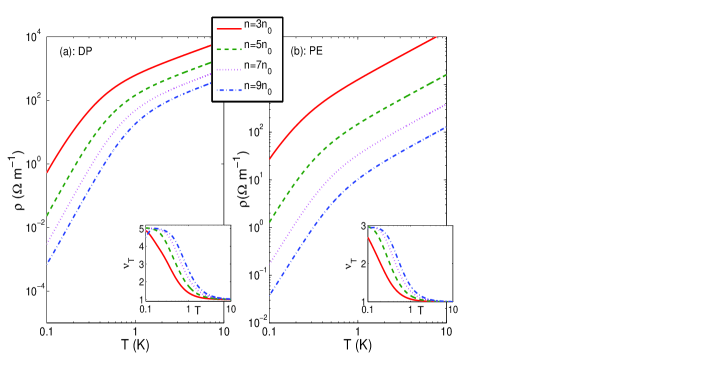
Figure 1: (Color online) The dependence of phonon limited resistivity on temperature is shown. Panel (a) and (b) represent DP and PE scattering contribution, respectively. Different values of density namely $n=3n_{0}$, $5n_{0}$, $7n_{0}$, and $9n_{0}$ are considered. The strength of RSOI is fixed to $\alpha=3\alpha_{0}$. The temperature variations of the exponent $\nu_{T}$ are shown in the insets of both panels.

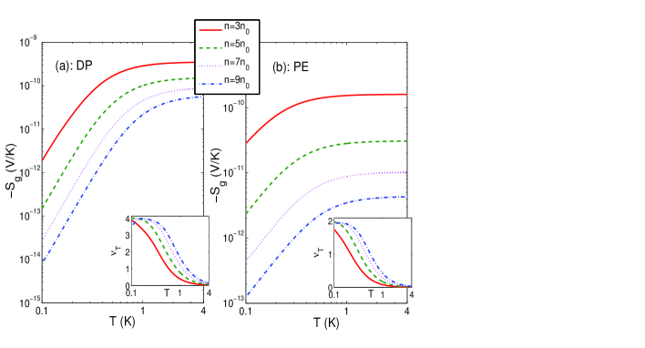
Figure 2: (Color online) Temperature dependence of phonon-drag thermopower due to DP and PE scatterings are shown. Different values of density namely $n=3n_{0}$, $5n_{0}$, $7n_{0}$, and $9n_{0}$ are considered. The strength of RSOI is fixed to $\alpha=3\alpha_{0}$. The temperature dependencies of the effective exponent of phonon-drag thermopower are shown in the insets of both panels.

For the numerical calculation following material parameters, appropriate for an InAs quantum wire, have been considered: $m^{\ast}=0.036m_{e}$ with free electron mass $m_{e}$, $g^{\ast}=-8$, $\rho_{m}=5.68\times 10^{3}$ Kg m^-3, $v_{sl}=4.41\times 10^{3}$ ms^-1, $v_{st}=2.35\times 10^{3}$ ms^-1, $D=-5.08$ eV, $h_{14}=3.5\times 10^{8}$ Vm^-1, $n_{0}=10^{7}$ m^-1, $R_{0}=10$ nm, and $\alpha_{0}=10^{-11}$ eVm. The value of the external magnetic field is taken to be $B=0.3$ T.

Fig. 1 shows the temperature variation of phonon limited resistivity for different densities namely $n=3n_{0},5n_{0},7n_{0}$ and $9n_{0}$. The value of Rashba parameter is considered as $\alpha=3\alpha_{0}$. Fig. 1 clearly demonstrates a crossover from the low temperature BG regime to high temperature equipartition regime (in which $\rho\sim T$). For both DP and PE scattering mechanisms $\rho$ decreases as $n$ increases. The resistivity due to PE scattering is higher in magnitude than DP scattering. The exponent $\nu_{T}$ of the temperature dependence of $\rho$ can be defined as $\nu_{T}=d{\rm{log}}\rho/d{\rm log}T$ which is extracted numerically and its variation with temperature has been shown in the insets of Fig. 1. It is clear that the temperature variation of $\nu_{T}$ depends on electron density. At lower density, namely $n=3n_{0}$ the exponent $\nu_{T}$ shows a clear deviation from the limiting case (i.e. $\nu_{T}=5$ due to DP and $\nu_{T}=3$ for PE scattering). As density increases the BG temperature regime becomes more stable. This numerically obtained BG regime is in excellent agreement with the approximated analytical results. As temperature increases $\nu_{T}$ approaches to its equipartition value i.e. $\nu_{T}=1$.

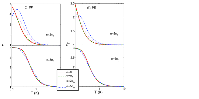
Figure 3: (Color online) The temperature variation of the effective exponent of resistivity i.e. $\nu_{T}=d{\rm log}\rho/d{\rm log}T$ for various values of $\alpha$, namely, $\alpha=0$, $\alpha_{0}$, $3\alpha_{0}$ and $5\alpha_{0}$ are shown. Left panel is considered for DP scattering in which upper and lower panel correspond to $n=2n_{0}$ and $6n_{0}$. Similarly right panel describes PE scattering for $n=2n_{0}$ and $6n_{0}$.

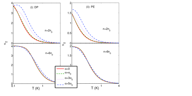
Figure 4: (Color online) The temperature variation of the effective exponent of phonon-drag thermopower i.e. $\nu_{T}=d{\rm log}S_{g}/d{\rm log}T$ for various values of $\alpha$, namely, $\alpha=0$, $\alpha_{0}$, $3\alpha_{0}$ and $5\alpha_{0}$ are shown. Left panel is considered for DP scattering in which upper and lower panel correspond to $n=2n_{0}$ and $6n_{0}$. Similarly right panel describes PE scattering for $n=2n_{0}$ and $6n_{0}$.

In Fig. 2 we show the temperature dependence of phonon-drag thermopower due to DP and PE scattering. $S_{g}$ decreases with the increase of density. In this case we also extract the exponent $\nu_{T}=d{\rm log}S_{g}/d{\rm log}T$ of the temperature dependence of $S_{g}$. Similar to the resistivity case the temperature dependence of $\nu_{T}$ also depends on the density as depicted in the insets. At higher density BG regime is obtained in which $S_{g}\sim T^{4}$ due to DP and $S_{g}\sim T^{2}$ due to PE scattering. The magnitude of $S_{g}$ due PE scattering is higher than that of DP scattering.

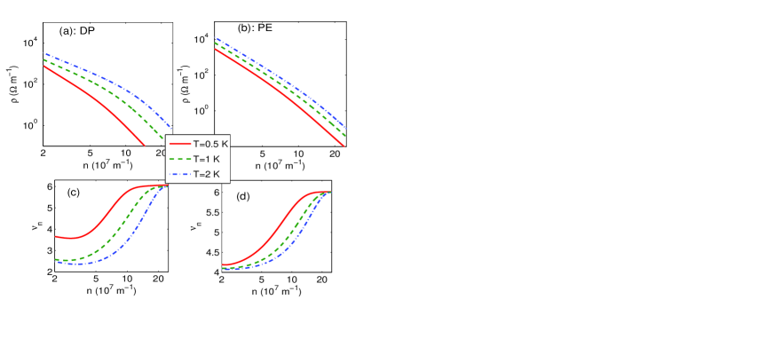
Figure 5: (Color online) The dependence of phonon limited resistivity on carrier density for different temperatures namely, $T=0.5$ K, $1$ K, and $2$ K are shown. We consider $\alpha=2\alpha_{0}$. Panels (a) and (b) are due to DP and PE scattering. In panels (c) and (d) we show the variation of the quantity $\nu_{n}=-d{\rm log}\rho/d{\rm log}n$ with $n$ due to DP and PE scattering respectively.

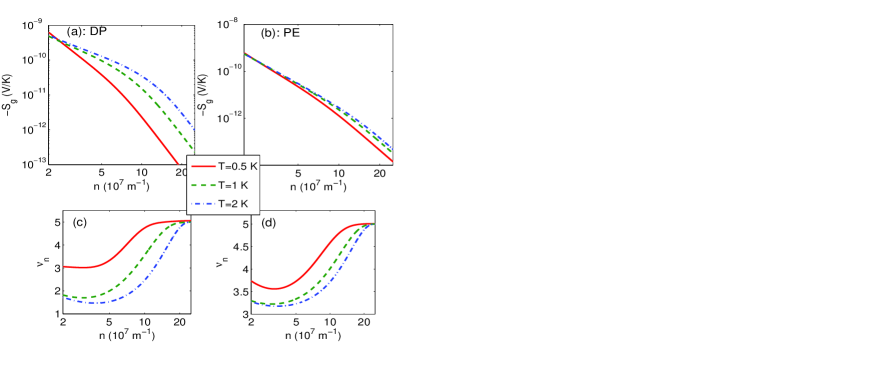
Figure 6: (Color online) The dependence of phonon-drag thermopower on carrier density for different temperatures namely, $T=0.5$ K, $1$ K, and $2$ K are shown. We consider $\alpha=2\alpha_{0}$. Panels (a) and (b) are due to DP and PE scattering. In panels (c) and (d) we show the variation of the quantity $\nu_{n}=-d{\rm log}S_{g}/d{\rm log}n$ with $n$ due to DP and PE scattering respectively.

Let us now discuss the following important point. The boundary of the BG regime is defined by the characteristic temperature $T_{BG}=2\hbar v_{s}k_{F}/k_{B}$. For a typical value of electron density, say $n=5n_{0}$ we have $T_{BG}\sim 6$ K. But it is obtained numerically that the BG regime exists for a small range of temperature below $1$ K.

The temperature dependence of $\nu_{T}$ not only depends on the density but also on the Rashba parameter $\alpha$. These facts are depicted in Figs. 3 and 4 in which the temperature dependencies of $\nu_{T}$ corresponding to $\rho$ and $S_{g}$ for different $\alpha$ are shown. When density is low the temperature variation depends significantly on $\alpha$. At a relatively higher density, the effect of $\alpha$ on this temperature dependence is not so prominent for both $\rho$ and $S_{g}$. Similar effect of $\alpha$ on the temperature dependence of $\rho$ or $S_{g}$ in a Rashba spin-orbit coupled two dimensional electron gas in BG regime has been addressed recently.tutul1 ; tutul2

In Figs. (5) and (6) we have shown how $\rho$ and $S_{g}$ depend on the electron density at a fixed temperature in BG regime. In Eqs. (23-25) and (28-30) one can notice that both IRT (and consequently $\rho$) and phonon-drag thermopower show a power law dependence with electron density through the Fermi wave vectors at a fixed temperature. So in general we can write $\rho$ or $S_{g}\sim n^{-\nu_{n}}$, where the exponent $\nu_{n}$ corresponding to $\rho$ and $S_{g}$ can be obtained by taking negative logarithmic differentiation of $\rho$ or $S_{g}$ with respect to $n$ i.e. $\nu_{n}=-d{\rm log}\rho(S_{g})/d{\rm log}n$. Let us now estimate $\nu_{n}$ from Eqs. (23-25) and (28-30). It is well known that the Fermi wave vector scales with density as $k_{F}^{0}\sim n$ in one dimension. In our case $k_{F}^{\lambda}$ depends on density in a complicated way as seen from Eq. (5). Nevertheless, we can find $k_{F}^{\lambda}\sim n$ since $k_{\alpha},\Delta/\alpha\ll 2m^{\ast}\epsilon_{F}/\hbar^{2}$. From Eqs. (23-25) one finds $\langle\tau^{-1}\rangle\sim n^{-5}$ and as a result we have $\rho\sim n^{-6}$. The phonon-drag thermopower depends on density as $S_{g}\sim n^{-5}$ as seen from Eqs. (28-30). However solving Eqs. (17) and (21) numerically we find that $\nu_{n}$ undergoes a crossover from a relatively lower density behavior to a higher density behavior for both $\rho$ and $S_{g}$. As density increases $\nu_{n}$ approaches towards the values obtained from asymptotic expressions i.e. $\nu_{n}=6$ for $\rho$ and $\nu_{n}=5$ for $S_{g}$. Note that at higher density same values of $\nu_{n}$ are obtained due to DP and PE scattering for both case of $\rho$ and $S_{g}$. But at lower densities $\nu_{n}$ differs significantly due to DP and PE scattering.

Although a gap $\Delta$ is considered in the energy spectrum but its magnitude is much smaller than that corresponding to the Rashba spin-splitting i.e. $\Delta\ll\alpha k_{F}$. The main purpose for considering $\Delta$ is to see whether inter-branch transitions are happening or not. But in the BG regime, the possibility of inter-branch scattering has been ruled out. So the qualitative results do not change significantly due to the presence of $\Delta$ in the energy spectrum.

IV Summary

In summary we have studied various features of acoustic phonon limited resistivity and phonon-drag thermopower in a Rashba spin-orbit coupled semiconductor QW with an in-plane magnetic field induced gap. Two mechanisms of electron-phonon interaction, namely, DP and PE scatterings are taken into consideration. In the BG regime a power law dependence of both resistivity and phonon-drag thermopower with temperature have been obtained analytically. We find the exponent ($\nu_{T}$) of the temperature dependence which takes the value $5$ and $3$ corresponding to the DP and PE scattering, respectively in the case of resistivity. $\nu_{T}$ becomes $4$ and $2$ in the case of phonon-drag thermopower due to DP and PE scattering, respectively. Through a numerical calculation, we have shown a transition in resistivity from BG to equipartition regime. Numerically, it is also found that $\nu_{T}$ depends on both density and Rashba parameter. At higher density $\nu_{T}$ matches well with that obtained from the analytical calculation for both $\rho$ and $S_{g}$ or in other words a BG regime is established at higher density. The effect of spin-orbit interaction on $\nu_{T}$ is found to be more prominent in low density regime. Finally the dependence of $\rho$ and $S_{g}$ on the carrier density are also discussed. An approximate analytical calculation shows that $\rho\sim n^{-6}$ and $S_{g}\sim n^{-5}$ in the BG regime. These dependence on $n$ have been confirmed through a numerical analysis at higher densities. The results obtained in the present case have also been compared with the corresponding results for spin-orbit coupled two-dimensional electron system and we obtain in both cases $S_{g}\rho^{-1}\sim T^{-1}$ which affirms Herring’s law.

Appendix A

In this Appendix we shall perform an explicit derivation of the term $\delta(\epsilon_{k_{F}\pm q}^{\lambda}-\epsilon_{k_{F}}^{\lambda}\mp\hbar\omega_{Q})$ as given in Eq. (16.)

From Eq. (2) one can write

$$\epsilon_{k_{F}+q}^{\lambda}=\frac{\hbar^{2}(k_{F}^{\lambda}+q)^{2}}{2m^{\ast}}+\lambda\sqrt{\alpha^{2}(k_{F}^{\lambda}+q)^{2}+\Delta^{2}}.$$ (32)

Now defining $\varepsilon_{k_{F}^{\lambda}}=\sqrt{(\alpha k_{F}^{\lambda})^{2}+\Delta^{2}}$ and assuming $q\ll k_{F}^{\lambda}$, the second term in Eq. (32) can be expanded up to $q^{2}$ as

$$\varepsilon_{{k_{F}^{\lambda}}+q}=\varepsilon_{k_{F}^{\lambda}}+\frac{\alpha^{2}k_{F}^{\lambda}q}{\varepsilon_{k_{F}^{\lambda}}}+\frac{\alpha^{2}q^{2}}{2\varepsilon_{k_{F}^{\lambda}}}\Big{(}1-\frac{\alpha^{2}k_{F}^{\lambda^{2}}}{\varepsilon_{k_{F}^{\lambda}}^{2}}\Big{)}.$$ (33)

We then have

$$\epsilon_{k_{F}+q}^{\lambda}-\epsilon_{k_{F}}^{\lambda}=\frac{\hbar^{2}}{2m^{\ast}}\tilde{g}_{\alpha}^{\lambda}\Big{(}q^{2}+2q\frac{\tilde{k}_{F}^{\lambda}}{\tilde{g}_{\alpha}^{\lambda}}\Big{)},$$ (34)

where $\tilde{g}_{\alpha}^{\lambda}$ and $\tilde{k}_{F}^{\lambda}$ are defined earlier.

Since we are dealing with the BG regime in which $q\ll k_{F}^{\lambda}$, the term $q^{2}$ in Eq. (34) can be neglected. So from the energy conservation $\epsilon_{k_{F}\pm q}^{\lambda}-\epsilon_{k_{F}}^{\lambda}\mp\hbar\omega_{Q}=0$, one can obtain $q=\big{(}m^{\ast}v_{s}/\hbar\tilde{k}_{F}^{\lambda}\big{)}Q$ with $Q=\sqrt{q_{\bot}^{2}+q^{2}}$. Since the coefficient $m^{\ast}v_{s}/(\hbar\tilde{k}_{F}^{\lambda})\ll 1$ and consequently we have $q\ll Q$ which in turn forces us to write the following expression

$$q=\frac{m^{\ast}v_{s}}{\hbar\tilde{k}_{F}^{\lambda}}q_{\bot}.$$ (35)

We now calculate the delta function corresponding to the absorption case which can be obtained in the following form

$$\delta(\epsilon_{k_{F}+q}^{\lambda} - \epsilon_{k_{F}}^{\lambda}-\hbar\omega_{Q})=\frac{2m^{\ast}}{\hbar^{2}\tilde{g}_{\alpha}^{\lambda}}\delta\Big{(}q^{2}+2q\frac{\tilde{k}_{F}^{\lambda}}{\tilde{g}_{\alpha}^{\lambda}}-\frac{2m^{\ast}v_{s}q_{\bot}}{\hbar\tilde{g}_{\alpha}^{\lambda}}\Big{)}$$ (36)

$$= \frac{2m^{\ast}}{\hbar^{2}\tilde{g}_{\alpha}^{\lambda}}\frac{1}{|q_{+}-q_{-}|}\Big{\{}\delta(q-q_{+})+\delta(q-q_{-})\Big{\}},$$

where $q_{\pm}=\Big{(}-\tilde{k}_{F}^{\lambda}+\sqrt{\tilde{k}_{F}^{\lambda^{2}}+C^{\lambda}q_{\bot}}\Big{)}/\tilde{g}_{\alpha}^{\lambda}$ with $C^{\lambda}=2m^{\ast}v_{s}\tilde{g}_{\alpha}^{\lambda}/\hbar$. With the approximation $q\ll k_{F}^{\lambda}$ one can find $q_{+}=m^{\ast}v_{s}q_{\bot}/(\hbar\tilde{k}_{F}^{\lambda})$ and $q_{-}=-2\tilde{k}_{F}^{\lambda}/\tilde{g}_{\alpha}^{\lambda}-m^{\ast}v_{s}q_{\bot}/(\hbar\tilde{k}_{F}^{\lambda})$. Since we are considering BG regime then one may ignore the term $\delta(q-q_{-})$ in Eq. (36). Exactly similar analysis can be done for emission case. Now it is straightforward to obtain Eq. (16) from Eq. (36).

References

- (1) D. D. Awschalom and M. E. Flatte, Nat. Phys. 3, 153 (2007).
- (2) S. A. Wolf, D. D. Awschalom, R. A. Buhrman, J. M. Daughton, S. von Molnar, M. L. Roukes, A. Y. Chtchelkanova, and D. M. Treger, Science 294, 1488 (2001).
- (3) R. Winkler, Spin-Orbit Coupling Effects in Two-Dimensional Electron and Hole Systems (Springer Verlag-2003).
- (4) I. Zutic, J. Fabian, and S. Das Sarma, Rev. Mod. Phys. 76, 323 (2004).
- (5) F. Fabian, A. Matos-Abiague, C. Ertler, P. Stano, and I. Zutic, Acta Physica Slovaca 57, 565 (2007).
- (6) Y. A. Bychkov and E. I. Rashba, J. Phys. C: Solid State Phys. 17, 6039 (1984).
- (7) J. Nitta, T. Akazaki, H. Takayanagi, and T. Enoki, Phys. Rev. Lett. 78, 1335 (1997).
- (8) T. Matsuyama, R. Kursten, C. Meibner, and U. Merkt Phys. Rev. B 61, 15588 (2000).
- (9) G. Dresselhaus, Phys. Rev. 100, 580 (1955).
- (10) S. D. Ganichev et. al., Phys. Rev. Lett. 92, 256601 (2004); S. Giglberger et. al., Phys. Rev. B 75, 035327 (2007).
- (11) J. Schliemann, J. C. Egues, and D. Loss, Phys. Rev. Lett. 90, 146801 (2003).
- (12) B. J. van Wees, H. van Houten, C. W. J. Beenakker, J. G. Williamson, L. P. Kouwenhoven, D. van der Marel, and C. T. Foxon, Phys. Rev. Lett. 60, 848 (1988).
- (13) F. Mireles and G. Kirczenow, Phys. Rev. B 64, 024426 (2001).
- (14) S. Datta and B. Das, Appl. Phys. Lett. 56, 665 (1990).
- (15) P. Streda and P. Seba, Phys. Rev. Lett. 90, 256601 (2003).
- (16) R. G. Pereira and E. Miranda, Phys. Rev. B 71, 085318 (2005).
- (17) R. M. Lutchyn, J. D. Sau, and S. Das Sarma, Phys. Rev. Lett. 105, 077001 (2010).
- (18) Y. Oreg, G. Refael, and F. von Oppen, Phys. Rev. Lett. 105, 177002 (2010).
- (19) L. Mao, M. Gong, E. Dumitrescu, S. Tewari, and C. Zhang, Phys. Rev. Lett. 108, 177001 (2012).
- (20) C. Kloeffel, M. Trif, and D. Loss, Phys. Rev. B 84, 195314 (2011).
- (21) C. H. L. Quay, T. L. Hughes, J. A. Sulpizio, L. N. Pfeiffer, K. W. Baldwin, K. W. West, D. Goldhaber-Gordon, and R. de Picciotto, Nat. Phys. 6, 336 (2010).
- (22) H. L. Stormer, L. N. Pfeiffer, K. W. Baldwin, and K. W. West, Phys. Rev. B 41, 1278 (1990).
- (23) P. J. Price, Ann. Phys. (NY) 133, 217 (1981); J. Vac. Sci. Technol. 19, 599 (1981); Surf. Sci. 113, 199 (1982); Surf. Sci. 143, 145 (1984); Solid State Commun. 51, 607 (1984).
- (24) B. K. Ridley, J. Phys. C: Solid State Phys. 15, 5899 (1982).
- (25) T. Kawamura and S. Das Sarma, Phys. Rev. B 45, 3612 (1992).
- (26) J. Lee and M. O. Vassell, J. Phys. C: Solid State Phys. 17, 2525 (1984).
- (27) G. Fishman, Phys. Rev. B 36, 7448 (1987).
- (28) U. Bockelmann and G. Bastard, Phys. Rev. B 42, 8947 (1990).
- (29) B. R. Nag and S. Gangopadhyay, Semicond. Sci. Technol. 10, 813 (1995).
- (30) V. Karpus and D. Lehmann, Semicond. Sci. Technol. 12, 781 (1997).
- (31) D. G. Cantrell and P. N. Butcher, J. Phys. C 19, L429 (1986); J. Phys. C 20, 1985 (1987); J. Phys. C 20, 1993 (1987).
- (32) S. S. Kubakaddi and P. N. Butcher, J. Phys.: Condens. Matter 1, 3939 (1989).
- (33) M. Tsaousidou and P. N. Butcher, Phys. Rev. B 56, R10044(R) (1997).
- (34) S. K. Lyo and D. Huang, Phys. Rev. B 66, 155307 (2002).
- (35) S. S. Kubakaddi, Phys. Rev. B 75, 075309 (2007).
- (36) T. Biswas and T. K. Ghosh, J. Phys.: Condens. Matter 25, 035301 (2013).
- (37) T. Biswas and T. K. Ghosh, J. Phys.: Condens. Matter 25, 265301 (2013); J. Phys.: Condens. Matter 25, 415301 (2013).
- (38) M. Governale and U. Zulicke, Solid State Commun. 131, 581 (2004).
- (39) Y. V. Pershin, J. A. Nesteroff, and V. Privman, Phys. Rev. B 69, 121306(R) (2004).
- (40) J. E. Birkholz and V. Meden, J. Phys.: Condens. Matter 20, 085226 (2008).
- (41) J. Lee and H. N. Spector, J. Appl. Phys. 57, 366 (1985).
- (42) G. Fishman, Phys. Rev. B 34, 2394 (1986).
- (43) C. Herring, Phys. Rev. 96, 1163 (1954).