Monopole and dipole estimation for multi-frequency sky maps by linear regression

We describe a simple but efficient method for deriving a consistent set of monopole and dipole corrections for multi-frequency sky map data sets, allowing robust parametric component separation with the same data set. The computational core of this method is linear regression between pairs of frequency maps, often called “T-T plots”. Individual contributions from monopole and dipole terms are determined by performing the regression locally in patches on the sky, while the degeneracy between different frequencies is lifted whenever the dominant foreground component exhibits a significant spatial spectral index variation. Based on this method, we present two different, but each internally consistent, sets of monopole and dipole coefficients for the 9-year WMAP, Planck 2013, SFD $100\thinspace\mu\textrm{m}$, Haslam 408 MHz and Reich & Reich 1420 MHz maps. The two sets have been derived with different analysis assumptions and data selection, and provides an estimate of residual systematic uncertainties. In general, our values are in good agreement with previously published results. Among the most notable results are a relative dipole between the WMAP and Planck experiments of 10–15$\thinspace\mu\textrm{K}$ (depending on frequency), an estimate of the 408 MHz map monopole of $8.9\pm 1.3\thinspace\textrm{K}$, and a non-zero dipole in the 1420 MHz map of $0.15\pm 0.03\thinspace\textrm{K}$ pointing towards Galactic coordinates $(l,b)=(308^{\circ},-36^{\circ})\pm 14^{\circ}$. These values represent the sum of any instrumental and data processing offsets, as well as any Galactic or extra-Galactic component that is spectrally uniform over the full sky.

1 Introduction

The cosmic microwave background (CMB) fluctuations consist of small variations with a root-mean-square (RMS) of $70\thinspace\mu\textrm{K}$ imprinted on top of a mean temperature of 2.73 K and a Doppler-induced dipole of $\sim$$3\thinspace\textrm{mK}$. These minute variations thus correspond to fractional fluctuations at the level of $\sim$$10^{-5}$ relative to the total signal. To minimize systematic uncertainties, modern CMB anisotropy experiments are therefore forced to employ some form of differential measuring technique, eliminating the large 2.73 K offset already at the instrument level. Both COBE-DMR (Smoot et al. 1992) and WMAP (Bennett et al. 2013) employed coupled differencing assemblies that only recorded temperature differences between two positions on the sky, while for Planck the instrumental offset is large and unknown, and cannot be used to constrain the monopole (Planck Coll. I 2013). However, while necessary for systematics suppression, this also implies that these experiments are intrinsically unable to measure the true absolute zero-point (or monopole) of their final maps. In addition, the dipole is also associated with a large relative uncertainty because of the large numerical value of the CMB Doppler dipole; a small relative error in the determination of the CMB dipole direction can induce a dipole error of many microkelvins in a CMB map. Typically, this will be strongly correlated among frequencies within a single experiment, though, and so informative priors can be imposed among frequency channels within a given experiment. For foreground-dominated frequency channels, instrumental systematics, such as gain fluctuations, may induce dipole errors.

Removing the monopole and dipole from CMB data sets does not constitute a major limitation in terms of CMB-based cosmological parameter analysis, since losing a handful harmonic modes out of many thousands only negligibly reduces the total amount of available information. However, it does have a significant indirect impact because of the presence of non-cosmological foreground contamination from Galactic and extra-Galactic sources. In order to obtain a clean image of the cosmological CMB fluctuations, this foreground contamination has to be removed from the raw sky maps through some form of component separation prior to power spectrum and parameter estimation. A wide range of such methods have been already been proposed (e.g., Planck Coll. XII 2013, and references therein), ranging from the simplest of template fitting and internal linear combination approaches through blind- or semi-blind image processing techniques to full-blown parametric Bayesian methods employing physical models. Except for the very simplest methods, all of these exploit the fact that all foreground frequency spectra are qualitatively different from the CMB spectrum. For instance, while the CMB spectrum is that of a perfect blackbody, thermal dust emission can be well approximated by that of a one- or two-component greybody. However, such relations clearly only hold if there are no arbitrary offsets between the different frequency maps. In other words, spurious monopole and dipole errors can bias any estimation algorithm that exploits frequency dependencies, and this can in turn lead to leakage between various components, and eventually contamination in the CMB estimate.

A number of methods have already been proposed in the literature for estimating monopoles, while fewer have addressed residual dipoles. One example of the former is the co-secant method adopted by the WMAP team (Bennett et al. 2003). In this case, the Galactic signal is approximated as plane-parallel in Galactic coordinates, with an amplitude falling roughly proportionally with the co-secant of the latitude. The major weakness of this method is that the Galaxy is neither plane-parallel nor follows a co-secant, and the method does also not account for residual dipole terms. A second approach was proposed by Eriksen et al. (2008), who include the monopole and dipole terms as additional free parameters within a global Bayesian parametric framework. The major weakness with this method is a large degeneracy between the monopole and dipole terms relative to the unknown zero-point of each foreground; it is possible to add a constant to each foreground amplitude, and then subtract a corresponding frequency-scaled offset from each monopole, leaving the net sum unchanged.

A third widely used method for setting the zero-level of radio maps is that of linear regression, or through so-called “T-T plots”. This method has a long and prominent history in radio astronomy (see, e.g., Turtle et al. 1962; Davies et al. 1996; Reich & Reich 1988; Reich et al. 2004; Wehus et al. 2013, and references therein), as it provides a highly robust estimate of the spectral index of a single signal component given observations at two different frequencies. When plotting the measured pixel values at one frequency as a function of the measured pixel values at the other frequency, the spectral index is given (up to a constant factor) by the slope of the resulting T-T plot, which is easily found by linear regression. The main virtue of this spectral index estimate is that it is completely insensitive to any constant offset in either of the two frequency maps, since these only affect the regression intercept, not the slope. Intuitively, offsets only shift the scatter plot horizontally or vertically, but they do not deform or rotate it.

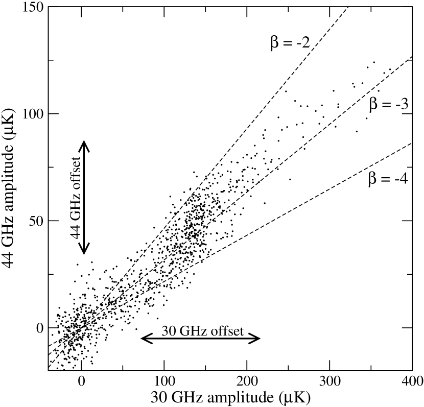
Figure 1: Schematic illustration of a single T–T plot evaluated for an ideal low-frequency Planck simulation (30 and 44 GHz). Each dot represents the observed values at two frequencies for a single pixel. The slope of the distribution is given by the spectral index of the signal component in the field, as indicated by the dashed lines. A constant offset in either frequency map simply translates the entire T–T plot either horizontally or vertically. For maps without spurious offsets, the best-fit straight line should pass through the origin; the fundamental idea of the algorithm presented in this paper is to ensure that this is the case for any sufficiently small patch of the sky.

In the following, we exploit the same idea to estimate both spurious monopoles and dipoles by noting that when the true values are correctly determined, the regression intercept has to be zero: If the foreground signal at one frequency is exactly zero, it also has to be exactly zero at the other frequency. This implies that a single T–T plot constrains both the spectral index of the component and the relative offsets of the two maps, $m_{1}$ and $m_{2}$, to $m_{1}=am_{2}+b$, where $a$ and $b$ are the slope and intercept of the T–T plot. The main goal of the present paper is to develop this simple idea into a complete and robust method for determining both monopoles and dipoles from a set of multi-frequency sky maps.

2 Method

Before describing the main method, we note that robust linear regression is in general difficult in the low signal-to-noise regime, as both the slope and intercept are associated with large uncertainties. We therefore adopt a two-step process in which we first use the main T–T plot method for high signal-to-noise frequency channels, followed by a direct template fit method for low signal-to-noise channels. The second stage, however, is both conceptually and implementationally straightforward and well established in the literature; the difficult task is to set the offsets correctly for the high signal-to-noise components, and this is our primary concern in the following.

2.1 Single region data model

We start by considering a basic data model consisting of a single signal component on the form

$$d_{\nu}(p)=F(\nu)s(p)+n_{\nu}(p)+m_{\nu},$$ (1)

where $d_{\nu}(p)$ denotes the observed sky map value at frequency $\nu$ and pixel $p$, $s$ represents the true sky signal (at some reference frequency, $\nu_{0}$), $F(\nu)$ denotes the (normalized) frequency spectrum of the sky signal (often called mixing matrix in the component separation literature), $n_{\nu}(p)$ is instrumental noise, and $m_{\nu}$ is the unknown spurious offset we want to estimate and remove. For now, $\mathbf{m}_{\nu}$ is taken to be a pure constant (monopole), and $F(\nu)$ is assumed constant over the entire observed field.

For many radio astronomy applications, the signal spectrum can be approximated by a power-law, $F(\nu)=(\nu/\nu_{0})^{\beta}$, at least over some limited frequency range. The effective spectral index, $\beta$, can be computed between any two frequencies, $\nu_{1}$ and $\nu_{2}$, using the so-called “T–T plot” technique. Let us first consider the noiseless case without offsets. For this case, the spectral index is given by

$$d_{2}=\left(\frac{\nu_{2}}{\nu_{1}}\right)^{\beta}d_{1}\Leftrightarrow\beta=\frac{\log\left(\frac{d_{2}}{d_{1}}\right)}{\log\left(\frac{\nu_{2}}{\nu_{1}}\right)}.$$ (2)

Defining the slope as $a\equiv(\nu_{2}/\nu_{1})^{\beta}$, and including noise and spurious offsets, this expression reads

$$d_{2}-(n_{2}+m_{2}) =a\left[d_{1}-(n_{1}+m_{1})\right]$$ (3)

$$d_{2} =ad_{1}+(m_{2}-a\thinspace m_{1})+(n_{2}-a\thinspace n_{1})$$ (4)

$$\equiv ad_{1}+b+n$$ (5)

Thus, the observed signal at one frequency is related linearly to signal at the other frequency, with a slope given uniquely by the spectral index, and an intercept given by $b\equiv(m_{2}-a\thinspace m_{1})$.

This relation is often conveniently visualized in terms of scatter (or “T–T”) plots, as illustrated in Fig. 1. Each dot indicates the observed data values at the two frequencies for one pixel, while the dashed lines indicate three models with different values of $\beta$. A spurious offset in either frequency map corresponds directly to a vertical or horizontal translation of the entire scatter plot, respectively, but does not change the slope. Therefore, the spectral index is fully insensitive to spurious constant offsets when estimated by this T–T plot technique. However, as shown below spurious dipoles do bias the spectral index, because they introduce a gradient across the field, resulting in a net additional tilt. The appropriate correction for this is discussed below.

As long as $F(\nu)\neq 0$ for all $\nu$, it is clear that if the data vanish in one frequency, it also have to disappear in the other. Thus, for data free of any spurious offsets the best-fit line through the T–T plot must pass through the origin. Correspondingly, a non-zero regression intercept can only be due to the offset term in Eq. 5, implying that $m_{1}$ and $m_{2}$ must be related by

$$m_{2}-a\thinspace m_{1}=b.$$ (6)

In other words, the true pair of offsets have to lie somewhere along the best-fit regression line in the T–T plot. From a single scatter plot it is impossible to determine the precise location, but this simple linear relation nevertheless forms the core unit of our algorithm.

Before proceeding with the algorithm, we make a few comments concerning the implementation of the fitting procedure for $a$ and $b$. First, since both $d_{1}$ and $d_{2}$ are noisy quantities, the standard method based on the normal equations does not strictly apply, as that estimator is known to suffer from so-called attenuation bias; noise in the descriptor variable, $d_{1}$, biases $a$ low (e.g., Draper & Smith 1998). Second, in real data sets strong outliers occur quite frequently; a typical example in the CMB setting is unmasked point sources. Since we will only apply this method to high signal-to-noise data sets in the following, the second problem is definitely more pressing for our purposes. We accordingly adopt the non-parametric and highly robust Theil-Sen estimator in the following (Theil 1950): We estimate the slope as $\hat{a}=\textrm{median}[(d_{2}(p_{2})-d_{2}(p_{1}))/(d_{1}(p_{2})-d_{1}(p_{1}))]$ evaluated over all pixel pairs $(p_{1},p_{2})$, and the intercept as $\hat{b}=\textrm{median}[d_{2}(p)-\hat{a}d_{1}(p)]$. If one wants to apply the same method to low signal-to-noise observations, a more appropriate estimator is the Deming estimator (Deming 1948), which properly accounts for uncertainties in both directions. We have implemented both of these estimators in our codes, and find fully consistent results for the cases considered in this paper.

2.2 Absolute monopole and dipole determination by spectral variations

Above we assumed that all pixels in the region of interest have the same spectral index, and the entire map may therefore be analyzed within a single T–T plot. In reality, the true spectral index varies across the sky to some extent. For instance, the spectral index of synchrotron emission typically ranges between, say, $\beta_{\textrm{s}}=-2.6$ and $-3.1$, while the thermal dust emissivity ranges between, say, $\beta_{\textrm{d}}=1.3$ and 1.8 (e.g., Planck Coll. XII 2013, and references therein). To account for these variations, it is therefore useful, if not necessary, to segment the sky map into disjoint regions such that the index can be approximated as nearly constant within each region. In the absence of a physically motivated segmentation algorithm, a good first-order approximation is simply to partition the sky into some coarse grid. For applications adopting the HEALPix pixelization (Górski et al. 2005), such as ours, the nested ordering scheme proves particularly useful for this purpose, as it allows fast and localized grid coarsening. For instance, while each sky map considered here are pixelized on a grid built up with $14{{}^{\scriptstyle\prime}}$ pixels (corresponding to a HEALPix resolution parameter of $N_{\textrm{side}}=256$), a single constant-index region is typically defined in terms of $3$ .${}^{\circ}8$ pixels ($N_{\textrm{side}}=16$), each containing $16\times 16$ high-resolution pixels.

Such partitioning into smaller regions is not only useful in order to ensure nearly constant spectral indices, but it allows in fact an absolute determination of the individual offsets, $m_{1}$ and $m_{2}$. Let the full data set be partitioned into $N$ regions, each with a (nearly) constant spectral index $\beta_{i}$, and perform an independent linear regression procedure for each region, as outlined above. In this case, one will obtain an independent linear constraint on $m_{1}$ and $m_{2}$, given by Eq. 6, from each region. These may be combined into the following (over-determined) linear system,

$$\left[\begin{array}[]{cc}-a_{1}&1\\ -a_{2}&1\\ \vdots&\\ -a_{N}&1\\ \end{array}\right]\left[\begin{array}[]{c}m_{1}\\ m_{2}\end{array}\right]=\left[\begin{array}[]{c}b_{1}\\ b_{2}\\ \vdots\\ b_{N}\end{array}\right]$$ (7)

Writing this linear system in a matrix form, $\mathbf{A}\mathbf{m}=\mathbf{b}$, it has a unique solution given by the normal equations, $\hat{\mathbf{m}}=(\mathbf{A}^{t}\mathbf{A})^{-1}\mathbf{A}^{t}\mathbf{b}$. Thus, any spatial variation in the spectral index breaks the degeneracy between the offsets at the two frequencies, and at least formally allows absolute determination of both.

2.3 Joint monopole and dipole determination

Partitioning the sky into sub-regions further allows us to estimate additional degrees of freedom. Specifically, suppose that the total offset parameter space may be spanned by some set of basis vectors, $T_{k}(p)$, each with an unknown amplitude, $z_{k}$. The archetypal example is the space spanned by a monopole and three dipoles, such that the total effective offset for a given frequency map is

$$\tilde{\mathbf{m}} =\mathbf{T}\mathbf{z}$$ (8)

$$=\left[\begin{array}[]{cccc}1&\cos\phi_{1}\thinspace\sin\theta_{1}&\sin\theta_{1}\sin\phi_{1}&\cos\theta_{1}\\ 1&\cos\phi_{2}\thinspace\sin\theta_{2}&\sin\theta_{2}\sin\phi_{2}&\cos\theta_{2}\\ \vdots&\vdots&\vdots&\vdots\\ 1&\cos\phi_{n}\thinspace\sin\theta_{n}&\sin\theta_{n}\sin\phi_{n}&\cos\theta_{n}\end{array}\right]\left[\begin{array}[]{c}z_{0}\\ z_{1}\\ z_{2}\\ z_{3}\end{array}\right],$$ (17)

where subscripts indicate pixel number. To account for these new degrees of freedom within a single region $i$, Eq. 6 generalizes to

$$\sum_{k=0}^{3}T_{k}(i)m_{k,2}-a\thinspace\sum_{k=0}^{3}T_{k}(i)m_{k,1}=b,$$ (18)

where we approximate the net impact of the additional templates as constant over the region, i.e., $T_{k}(i)=1/N_{\textrm{pix}}\sum_{p\in i}T_{k}(p)$. The full joint all-regions linear system, corresponding to Eq. 7, is correspondingly generalized into $\mathbf{A}\mathbf{x}=\mathbf{b}$, where $\mathbf{A}$ now is an $N\times 8$ matrix containing $-a_{i}T_{k}(i)$ for region $i$ and template component $k$ in the first four columns, and $T_{k}(i)$ in the four last columns. The $\mathbf{x}$ vector has 8 elements containing the template amplitudes for the first map in the first four entries, and the template amplitudes for the second map in the four last entries. The right-hand side, $\mathbf{b}$, is identical to that in Eq. 7. Again, this system is solved by the normal equations, $\hat{\mathbf{x}}=(\mathbf{A}^{t}\mathbf{A})^{-1}\mathbf{A}^{t}\mathbf{b}$.

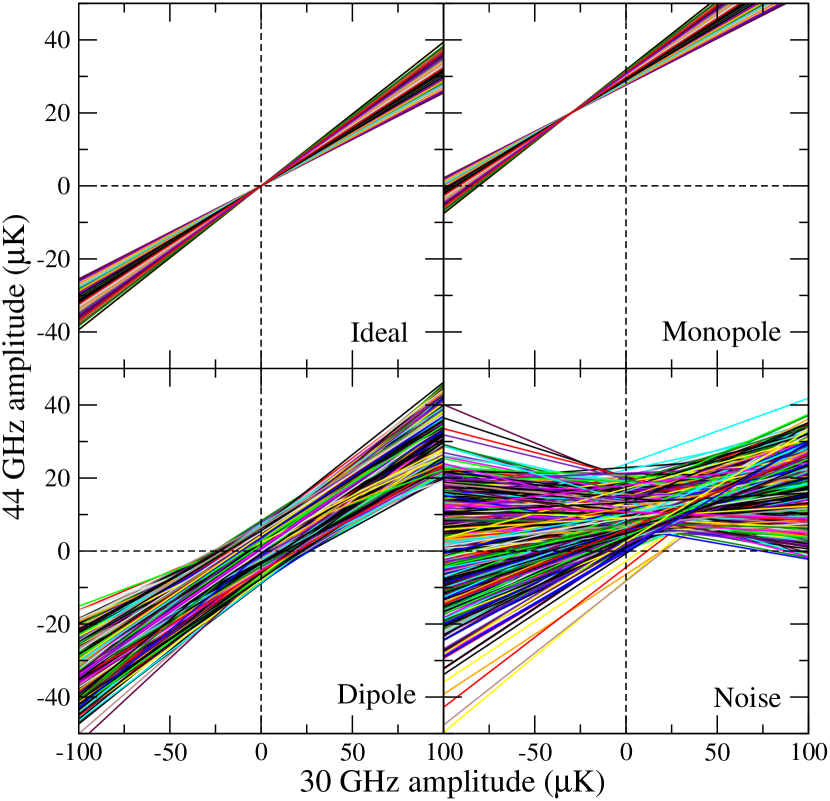
Figure 2: T–T summary plot of four different simulations. Each coloured line corresponds to the best-fit to a single HEALPix $N_{\textrm{side}}=8$ region, evaluated from underlying an $N_{\textrm{side}}=256$ synchrotron-only simulation. The top left panel shows the ideal case with neither spurious offsets nor instrumental noise; all lines converge perfectly on the origin. In the top right panel spurious offsets of $-30$ and +20$\thinspace\mu\textrm{K}$ are added to the two frequencies, resulting in a simple corresponding translation of the entire plot. The bottom left panel shows the effect of a spurious dipole; the lines no longer converge on a single point, as each region is effectively translated by a different offset. Finally, the bottom right panel illustrates the effect of instrumental noise.

While spurious monopoles do not change the net slope of a T–T plot, spurious dipoles do. And the larger area the considered region covers, the larger the effect is. We account for this effect by iteration. That is, we 1) solve Eq. 18 as described above, 2) subtract the derived monopole and dipole estimates from the raw input maps, and 3) iterate until all offset updates are smaller than, say, 1% of the total value. Typically three or four iterations are needed to reach convergence.

In Fig. 2 four different simulations illustrate the various cases discussed so far. Each line corresponds to the best-fit linear fit to the T–T plot of a synchrotron-only sky evaluated at 30 and 44 GHz, corresponding to the two lowest Planck frequencies. Each sky map has an angular resolution of $1^{\circ}$ FWHM, and is pixelized on an $N_{\textrm{side}}=256$ HEALPix grid. The spectral index is chosen to be constant within each $N_{\textrm{side}}=8$ pixel, and drawn from a Gaussian distribution with $\beta=-3\pm 0.2$, resulting in 768 independent T–T plots.

In the top left panel, we show the ideal case with neither spurious offsets nor instrumental noise. In this case, we see that all lines truly converge on the origin, as they should. In the top right panel we have added a $-30\thinspace\mu\textrm{K}$ offset to the 30 GHz channel, and a $+20\thinspace\mu\textrm{K}$ offset to the 44 GHz channel. The entire plot is translated accordingly, now focusing on the point $(d_{1},d_{2})=(-30,20)\thinspace\mu\textrm{K}$. Intuitively, the main goal of monopole correction is to re-center the focal point on the origin.

Next, the bottom left panel shows the effect of adding a spurious dipole to each frequency band. For a single region, this is almost equivalent to a simple translation, just like a monopole; however, each scatter plot is translated differently, depending on its position on the sky. When considering all T–T plots simultaneously, the overall distribution therefore appears smeared out, and possibly offset from the correct position, depending on the relative orientation between the two dipoles and the dominant Galactic signal. The intuitive goal of dipole correction is to make the focus point of this plot as sharp as possible.

Finally, the bottom right panel illustrates the effect of instrumental noise. This simply smears out each individual line, making it harder to assess where the lines converge to a single point. When the instrumental noise becomes comparable to the signal, robustly estimating the slopes and intercepts becomes very difficult, and we choose for now not to be aggressive in this respect; for low signal-to-noise cases, we find that simpler template fitting methods yield more robust results.

2.4 Preparing for real-world applications

The algorithm presented in the previous section constitutes the central engine in our method, and is already at this stage a self-contained and complete method for ideal data sets. However, real data are seldom ideal, and several adjustments and extensions are usually required before the method becomes practical. In this section we present a list of these issues, as well as their solutions.

2.4.1 Analyzing multi-resolution data sets

First, most multi-frequency data sets typically have different angular resolutions at different frequencies. In order to estimate the spectral indices (i.e., slopes) reliably across frequencies, it is therefore necessary to smooth all bands to a common angular resolution. To do so, we decompose each sky map into spherical harmonics, $d(p)=\sum_{\ell m}a_{\ell m}Y_{\ell m}(p)$. According to the spherical convolution theorem, a convolution in pixel domain translates into a multiplication in harmonic domain by the convolution theorem, such that if $b_{\ell}^{0}$ is the Legendre transform of the intrinsic instrumental beam, and $b_{\ell}$ is the Legendre transform of the desired common beam, the smoothed map is given by $\hat{d}(p)=\sum_{\ell m}(b_{\ell}/b_{\ell}^{0})a_{\ell m}Y_{\ell m}(p)$.

This degradation does not change the monopole or dipoles of the original map, and the derived low-resolution offset corrections can therefore be applied also to the full-resolution data set. However, it is important to note that information is lost in this process, in the sense that the T–T plots exhibits a smaller dynamic range after smoothing, effectively making it harder to pinpoint the optimal solution. One should therefore not smooth more than necessary to bring the frequency maps to a common resolution.

2.4.2 Joint analysis of multiple frequency bands

Second, many recent data sets have more than two frequency channels, whereas the T–T plot method intrinsically only involves pairs of maps. To deal with multiple maps, we order the maps according to frequency, and derive Eq. 7 for each pair of neighbouring frequencies. Considering the simplest case with only a monopole degree-of-freedom for each of $k$ frequency bands, this results in the following joint system,

$$\left[\begin{array}[]{ccccc}-a_{1}&1&0&\ldots&0\\ 0&-a_{2}&1&\ldots&0\\ 0&0&-a_{3}&\ldots&0\\ \vdots&\vdots&\vdots&\vdots&\vdots\\ 0&0&0&\ldots&1\end{array}\right]\left[\begin{array}[]{c}m_{1}\\ m_{2}\\ \vdots\\ m_{k}\end{array}\right]=\left[\begin{array}[]{c}b_{1}\\ b_{2}\\ \vdots\\ b_{k}\end{array}\right]$$ (19)

Generalization to dipole estimation and multiple regions is straightforward, although somewhat notationally involved. Note also, of course, that nothing prevents including frequency pairs beyond neighboring in the fit; the only limitation is that any given frequency pair should be well described by a single dominant signal component, which typically sets an effective limit on the allowed frequency range.

2.4.3 Subtracting CMB fluctuations

For frequencies between 30 and 143 GHz, the Planck and WMAP sky maps are dominated by CMB fluctuations rather than diffuse Galactic foregrounds. Over the cleanest regions of the sky, these fluctuations can therefore in principle serve as the signal for evaluating the scatter plot slopes and intercepts. However, this is non-trivial for at least two reasons. First, the CMB variance is typically of the order of $70\thinspace\mu\textrm{K}$ on degree angular scales, while both the desired offset precision and the instrumental noise are typically just a few microkelvins. Second, since the CMB frequency spectrum follows a blackbody, it has by definition a constant spectral index (equal to 0) at all frequencies and positions on the sky. Offset estimation on CMB fluctuations therefore give at most relative results, and even those are associated with relatively large uncertainties.

The most straightforward solution, and the one adopted in the following, is to subtract an estimate of the CMB sky (e.g., Planck Coll. XII 2013; Bennett et al. 2013) from all sky maps prior to offset estimation. The accuracy of this estimate is not critical, as the nature of CMB fluctuations are very close to Gaussian, and they therefore mostly add random noise to the T–T plots. As long as the CMB uncertainties are significantly smaller than the absolute foreground amplitude of the relevant channel, which usually is the case with current CMB experiments, the fit is stable. However, in order to ensure that the resulting offset correction estimates are directly applicable to the original sky maps, one should ensure that whatever CMB estimate is subtracted is orthogonal to all basis vectors, $T_{k}$, which in practice implies making sure that it does not have any monopole or dipole components. However, an uncertainty in this estimate will in the end translate directly into an uncertainty with the very specific CMB frequency spectrum, and will therefore not confuse component separation algorithms, as long as these also allow for a monopole and dipole component in the CMB fit.

2.4.4 Handling multiple signal components by masking

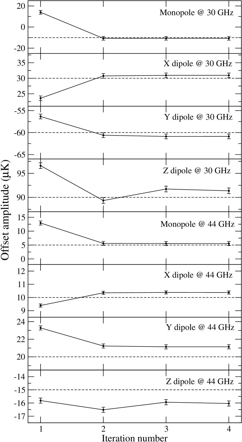
Figure 3: Recovered offset coefficients as a function of analysis iteration for a two-band simulation. The true input values are shown as dashed horizontal lines. The values change between iterations because spurious dipoles bias the slope of the T–T plots; iterative dipole correction remove this bias. Overall, the method reproduces the true input values to $\lesssim 1\thinspace\mu\textrm{K}$. However, the adopted bootstrap uncertainties tend to underestimate the uncertainties in the sub-dominant channels (44 GHz in this case), and are only intended to give an indication of the true uncertainties. End-to-end simulations are required for fully reliable uncertainty estimation.

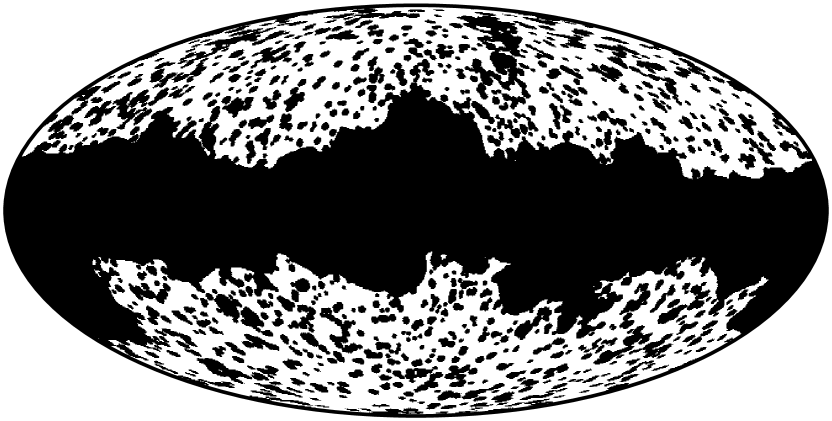
Figure 4: Joint mask used for the analysis of the WMAP, Planck and $100\thinspace\mu\textrm{m}$ maps.

                    

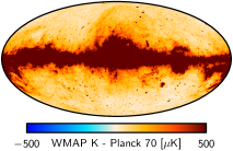
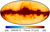
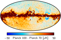
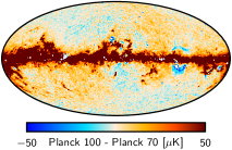
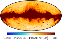
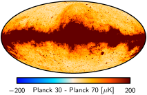
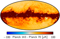
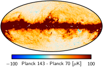
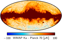
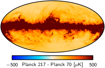
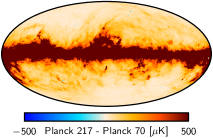
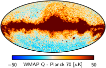
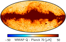
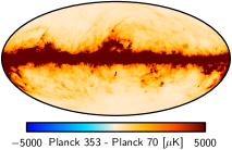
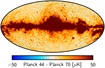
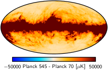
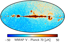
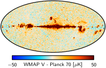
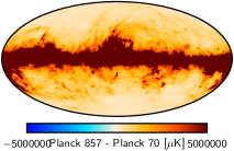
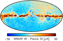
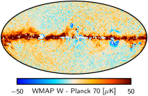
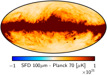
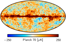
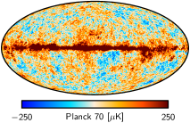
Figure 5: Difference maps between the CMB and high-frequency channels and the 70 GHz map, before (first and third columns) and after (second and fourth columns) offset corrections. The bottom row shows the pre- and post-correction 70 GHz map itself.

Related to the previous issue, the algorithm intrinsically assumes the presence of only one dominant foreground component per region. For data sets such as the low-frequency and synchrotron dominated 408 MHz Haslam and 1420 MHz Reich & Reich maps, this is for most parts of the sky not an issue. Neither is it for the high-frequency Planck channels above 143 GHz, which are dominated by thermal dust emission. However, for the low-foreground Planck and WMAP CMB channels between, say, 30 and 100 GHz somewhat greater care is warranted. For these frequencies, the overall signal budget is made up by a combination of synchrotron, free-free, anomalous microwave emission (AME; spinning dust), CO and thermal dust emission (Planck Coll. XII 2013). For some frequencies, this complication can be solved by masking, by removing spatially localized components such as CO and free-free. For other frequencies, say, between 20 and 40 GHz, where both synchrotron and AME are significant and not spatially localized, more sophisticated component separation methods should be used, simultaneously accounting for multiple components.

2.4.5 Template fitting near the foreground minimum

Near the foreground minimum around 70 GHz, low-frequency foregrounds (AME, free-free and synchrotron) and thermal dust contribute (by definition) equally, and the scatter plot technique is therefore intrinsically unreliable. In addition, the foreground signal-to-noise level is low, further destabilizing the T–T plot technique. On the other hand, the absolute foreground levels are also correspondingly low, and even simple methods are typically able to derive quite accurate monopole and dipole estimates. We therefore adopt the following template fitting technique for frequencies between 33 (WMAP Ka-band) and 100 GHz: we first derive absolute offset corrections for all high-foreground frequencies, and apply these to the respective (CMB-subtracted) channel maps. We then adopt the nearest neighbors on either side of the foreground minimum (i.e., the Planck 30 and 143 GHz maps) as low-frequency foreground and thermal dust templates, respectively. We then fit these together with the monopole and three dipoles to the low-foreground channels by solving the generalized normal equations,

$$\mathbf{z}=(\mathbf{T}^{T}\mathbf{N}^{-1}\mathbf{T})^{-1}\mathbf{T}^{T}\mathbf{N}^{-1}\mathbf{d},$$ (20)

where $\mathbf{T}$ is the $N_{\textrm{pix}}\times 6$ matrix listing each template column-wise, and $\mathbf{N}$ is the (assumed diagonal) pixel noise covariance matrix. A very conservative mask excluding both point sources and residual Galactic contamination is applied in the fit, as shown in Fig. 4.

We typically find that the uncertainties from this fit are on the order of a few microkelvins. However, even such small uncertainties can in principle be detected by detailed $\chi^{2}$ based analyses, for instance as implemented in parametric foreground methods like Commander (Eriksen et al. 2008). For such applications, we recommend that one fits (or at least verifies) the offset amplitudes for these channels within the joint analyses itself, accounting simultaneously for foreground amplitudes and overall offsets.

2.4.6 Stabilization by a positivity prior

To improve the rigidity and physicality of the fit, it can be advantageous to impose a positivity prior on the foreground amplitudes, by requiring that the post-correction frequency map is non-negative everywhere. We implement this as an optional feature in our codes as follows. We locate the coldest set of pixels on the sky, separated by at least $10^{\circ}$ on the sky. Each pixel value defines an independent inequality constraint on the offset coefficients given by

$$d(p)-\sum_{i=1}^{4}T_{i}(p)z_{i}\geq 0.$$ (21)

For cases with significant noise contribution, the inequality should be relaxed by adding $N\sigma(p)$ to the right-hand side, where $\sigma(p)$ is the instrumental noise RMS in pixel $p$, and $N$ is a threshold level in units of $\sigma$; we adopt $4\sigma$ as our positivity threshold. Note that optimization of, say, Eq. 19 under these constraints is a substantially computationally more complicated problem than solving the linear normal equations, and must be performed using non-linear methods.

2.4.7 Uncertainty estimation

Finally, we make a short note on estimation of statistical uncertainties, but emphasize that this topic is by far the most complicated part of the entire procedure, and the method outlined here is only intended to give a rough estimate of the uncertainties. The fundamental problem is that for most current experiments, the monopole and dipole coefficient uncertainties are vastly dominated by systematic effects (foreground modelling, optical imperfections etc.), rather than instrumental noise. Noise-based uncertainties are therefore virtually meaningless for describing true uncertainties. For this reason, we adopt a Monte Carlo based bootstrap method for now, aiming to capture some of these intrinsic systematic uncertainties in a non-parametric manner. From a data set consisting of $m$ disjoint sky regions, we select randomly a sub-sample of $m$ regions (i.e., one region may be included several times), and perform the full analysis on this sub-sample in the same manner as for the original data set. This process is repeated typically 100 times, and the resulting variance among those 100 resamples is taken as the bootstrap uncertainty. Further, any tunable parameter, such as whether to perform the analysis on $N_{\textrm{side}}=4$, 8 or 16 regions, are also drawn randomly within their allowed ranges between each resample.

The main advantage of this bootstrap approach is that it does to some extent account for foreground modelling uncertainties and algorithmic choices. However, it is still determined by the actually realized sky, and can therefore only account for those variables that vary within our actual data set; not those that are fixed for a given realization, but in principle stochastic. The method will therefore necessarily underestimate the true uncertainties, and we caution against interpreting these as Gaussian 68% confidence levels. For fully reliable uncertainty estimation, proper end-to-end simulations (including different foreground realizations in each simulation) are likely to be the only truly satisfactory solution, which is outside the scope of the current paper.

2.5 Analysis of a simple simulation

Table 1: Monopole and dipole estimates for two different analysis configurations. The top section summarizes the results for the main analysis of all 17 frequency maps considered in this paper, and the bottom section shows the results from the reduced 14 frequency data set employing external priors and different masks. Uncertainties are defined to be the maximum of the Monte Carlo-based bootstrap error described in Section 2.4 and $1\thinspace\mu\textrm{K}$. Conversion between Galactic Cartesian and polar coordinates is given by $(l,b)=(90^{\circ}-\textrm{acos}[Z/A],\textrm{atan2}[Y/A,X/A])$, where $A=\sqrt{X^{2}+Y^{2}+Z^{2}}$ is the dipole amplitude. Temperatures are given in thermodynamic units.

Sky map        Method        Partner(s)        Monopole        X dipole        Y dipole        Z dipole        Unit

17 band combination; tuned mask; no external priors

Haslam 408 MHz.        T–T fit        1420 MHz        $$8.9\kern 3.5pt\pm 1.3\kern 3.5pt$$                                K

R&R 1420 MHz.        T–T fit        408 MHz                                        K

WMAP K-band.        T–T fit        30 GHz                                        

WMAP Ka-band.        Template fit        30 + 143 GHz                                        

WMAP Q-band.        Template fit        30 + 143 GHz                                        

WMAP V-band.        Template fit        30 + 143 GHz                                        

WMAP W-band.        Template fit        30 + 143 GHz                                        

Planck 30 GHz.        T–T fit        K-band                                        

Planck 44 GHz.        Template fit        30 + 143 GHz                                        

Planck 70 GHz.        Template fit        30 + 143 GHz                                        

Planck 100 GHz.        Template fit        30 + 143 GHz                                        

Planck 143 GHz.        T–T fit        217 GHz                                        

Planck 217 GHz.        T–T fit        143 + 353 GHz                                        

Planck 353 GHz.        T–T fit        217 + 545 GHz                                        

Planck 545 GHz.        T–T fit        353 + 857 GHz                                        MJy/sr

Planck 857 GHz.        T–T fit        545 GHz + 100 m                                        MJy/sr

SFD 100 m.        T–T fit        857GHz                                        MJy/sr

14 band combination; WMAP KQ85 mask + ; fixed 353 GHz monopole and WMAP dipoles

Haslam 408 MHz.        T–T fit        1420 MHz                                        K

R&R 1420 MHz.        T–T fit        408 MHz                                        K

WMAP K-band.        T–T fit        30 GHz                                        

WMAP Ka-band.        T–T fit        30 GHz + Q-band                                        

WMAP Q-band.        T–T fit        Ka-band + 44 GHz                                        

WMAP V-band.        T–T fit        30 + 143 GHz                                        

WMAP W-band.        T–T fit        30 + 143 GHz                                        

Planck 30 GHz.        T–T fit        K-band                                        

Planck 44 GHz.        T–T fit        Q-band + V-band                                        

Planck 70 GHz.        T–T fit        V-band + W-band                                        

Planck 100 GHz.        T–T fit        W-band + 143 GHz                                        

Planck 143 GHz.        T–T fit        100 GHz + 217 GHz                                        

Planck 217 GHz.        T–T fit        143 + 353 GHz                                        

Planck 353 GHz.        T–T fit        217 GHz                                        

^a Dipoles fixed to official WMAP values.
^b 353 GHz monopole fixed by HI cross-correlation (Planck Coll. VII 2013).

Before applying our method to real observations, we analyze a simple well-controlled simulation, to check that the method produces sensible results in this case. Specifically, we once again consider a synchrotron-plus-noise simulation, with the signal component evaluated at the two lowest Planck frequencies, 30 and 44 GHz, but this time adopting the spatial spectral index distribution derived from the 408 and 1420 MHz maps in Sect. 4, and summarized in Fig. 9. In addition, we add spurious monopoles and dipoles to both maps ranging between $-60$ and +90$\thinspace\mu\textrm{K}$.

The results from this simulation are summarized in Fig. 3 for each offset parameter, as a function of analysis iteration. The dashed lines show the true value, and the uncertainties indicate the bootstrap errors described above. The general behaviour seen in this plot is typical for all cases we have analyzed, and therefore serves as a useful tool for building intuition about the performance of the method. First, and most importantly, we see that the method overall reproduces the true input values in terms of absolute values to a precision of at worst 1–$2\thinspace\mu\textrm{K}$.

Second, we see that the largest changes are observed between the first and the second iteration. This is due to the already mentioned fact that a spurious dipole introduces a bias in the effective slope (or spectral index) of the T–T plots, and this in turn leads to a leakage of dipole power into the monopole. However, even the first-order dipole correction leads to a vastly improved monopole estimate, and subsequently nearly stable results; the 30 GHz monopole jumps directly from +15$\thinspace\mu\textrm{K}$ to the true value of $-10\thinspace\mu\textrm{K}$ in the second iteration. Additional iterations only change the results with small amounts.

Third, as already stressed in Sect. 2.4, we see that the bootstrap uncertainties do not adequately describe the true uncertainties in the fit for all coefficients. While they do a reasonable job for the dominant 30 GHz channel, they underestimate the uncertainties at 44 GHz by up to a factor of four or five. However, it is again important to note that the absolute uncertainties for the same coefficients are small. In general, the bootstrap errors tend to produce a reasonable estimate for the dominant channels, but underestimate the uncertainties in the sub-dominant channels. In this paper, we will never quote uncertainties smaller than $1\thinspace\mu\textrm{K}$ for any component, even if the formal bootstrap uncertainty for a few cases is as low as $0.2\thinspace\mu\textrm{K}$.

3 Data and analysis setup

We now turn our attention to a set of 17 publicly available full-sky maps of the radio, millimeter and sub-millimeter sky, with the goal of establishing a consistent set of offset coefficients that can be used for multi-experiment CMB component separation analysis. We include in the following 1) the nine Planck 2013 temperature sky maps (Planck Coll. I 2013), ranging between 30 and 857 GHz; 2) the five 9-year WMAP temperature sky maps (Bennett et al. 2013) at K- (23 GHz), Ka- (33 GHz), Q- (41 GHz), V- (61 GHz) and W-band (94 GHz); 3) two low-frequency maps at 408 MHz (Haslam et al. 1982) and 1420 MHz (Reich 1982; Reich & Reich 1986; Reich et al. 2001), respectively; and 4) the $100\thinspace\mu\textrm{m}$ map by Schlegel et al. (1998). For Planck and WMAP we use the non-foreground cleaned co-added frequency maps; for the 408 MHz map, we use the version available on LAMBDA that has no filtering applied; and the $100\thinspace\mu\textrm{m}$ map accounts for the DIRBE and IRAS bandpasses. All maps are downgraded to a common resolution of $1^{\circ}$, and repixelized at a HEALPix resolution of $N_{\textrm{side}}=256$. No further corrections are applied to any map.

For the positivity prior, we need a rough estimate of the instrumental uncertainty per pixel. For WMAP and Planck  we base this on the provided high-resolution noise variance maps. For the two low-frequency and the $100\thinspace\mu\textrm{m}$ channels we enforce a strict positivity prior, and simply demand that there should be no negative pixels at all.

The 408 and 1420 MHz maps are analyzed together, and separately from the other 15 maps, which are all analyzed jointly. For the low-frequency analysis, we adopt the WMAP KQ85 mask (Bennett et al. 2013), and for the main analysis we additionally apply the Planck GAL60 Galactic and PCCS+SZ point source mask (Planck Coll. XII 2013). This joint mask is first smoothed by a $10^{\prime}$ Gaussian beam, and thresholded at a value of 0.5, to remove the very smallest source holes from the Planck mask. Then it is smoothed by a $1^{\circ}$ Gaussian beam, and thresholded at 0.99, to exclude residual foregrounds leaking out of the mask after smoothing each frequency map to the common resolution of $1^{\circ}$. The resulting mask is shown in Fig.  4, and permits a total of 38 % of the sky.

We use the main T–T scatter plot technique for the 408–1420 MHz combination, as well as for the combination of WMAP K-band and Planck 30 GHz and for all frequencies above 143 GHz. For the frequencies between WMAP Ka-band and Planck 100 GHz we use the template fit technique described in Sect. 2.4, and adopt the Planck 30 and 143 GHz channels as foreground tracers for low-frequency foregrounds and thermal dust, respectively. For CMB suppression, we adopt the Planck Commander solution from which the monopole and dipole has been removed outside the Commander analysis mask (Planck Coll. XII 2013). For robustness, we also performed an analysis using the low-foreground 9-year WMAP ILC CMB map (Bennett et al. 2013), obtaining nearly identical results.

To explore overall stability with respect to analysis choices, we additionally analyze a subset of the above. As reported by Planck Coll. XII (2013), the spectral index of thermal dust below 353 GHz is found to be lower than the expected value of 1.3–1.7 over extended regions of the sky. This may be explained either in terms of systematic uncertainties in the maps, or a break in the spectral index around 353 GHz, or simply a general break-down of the simple one-component greybody model. When including the high-frequency channels, as done above, this feature is regularized by high signal-to-noise measurements, resulting in a far more stable fit. However, this stability comes at a cost; if there happens to exist a second thermal dust component, the scatter plot technique is not well defined. In this case, it would be better for the low-frequency channels to exclude the high-frequency channels, and thereby reduce the overall sensitivity to this second component. The second data set considered here therefore comprises the 14 frequency bands up to (and including) the Planck 353 GHz channel. However, as noted by Planck Coll. XII (2013), this does result in a large uncertainty for the 353 GHz monopole. Therefore, we additionally fix this number to $308\thinspace\mu\textrm{K}$, a value determined by Planck Coll. VII (2013) through cross-calibration with HI observations.

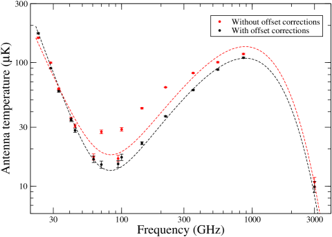
Figure 6: Mean antenna temperature as a function of frequency, measured outside the union mask before (red points) and after (black points) offset corrections. The dashed lines shows the best-fit sum of a low-frequency power-law (with free spectral index) and a one-component greybody (with fixed emissivity of $\beta_{\textrm{d}}=1.6$ and temperature $T_{\textrm{K}}=18\thinspace\textrm{K}$; Planck Collaboration XI 2013; Planck Collaboration XII 2013; Planck Collaboration Int. XVII 2014; Planck Collaboration Int. XXII 2014) to each of the two cases.

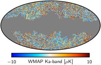
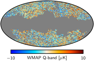
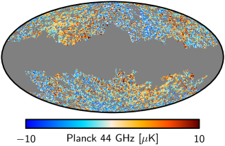
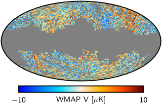
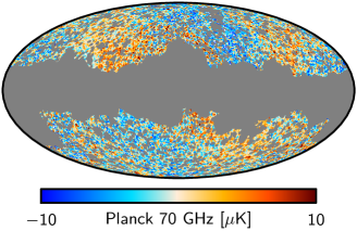
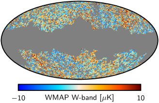
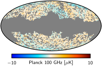
Figure 7: Map residuals after subtracting the best-fit template set (CMB, monopole, dipole, synchrotron/30 GHz and thermal dust/143  GHz).

We make three additional changes for this particular analysis. First, we fix the WMAP dipoles to zero, recognizing that the WMAP scanning strategy should be well suited to measure this particular mode. Second, to probe sensitivity to sky coverage, we impose a less conservative sky cut consisting only of the union of the WMAP KQ85 mask and a straight $|b|>25^{\circ}$ mask, in total allowing 54% of the sky. In this case, we use the T–T plot technique for all frequencies.

Analogous to fixing the WMAP dipole to zero in the consistency run, it is of course simple to impose additional external constraints whenever available, and these will always improve the rigidity of the overall fit. For example, the dominant source of dipole uncertainty for the CMB-dominated channels is the CMB dipole itself, as indeed is demonstrated in the following. In these cases, one may therefore impose a sharp prior on the dipole direction by including only a single dipole template in Eq. 18, with a direction equal to the CMB dipole. A second example are the high-frequency channels above 353 GHz, which are strongly signal dominated and may be assumed to have lower relative dipole errors than the CMB channels. Imposing a zero prior on these components may be justifiable. However, in this paper, we fit explicitly for all components without such priors, both to demonstrate the method and to derive minimal-assumption and conservative estimates for all channels.

4 Results

A complete summary of our main results is presented in Table 1, listing the monopole and dipole coefficients for all sky maps considered in the analysis. The top section shows the results from the main 17 frequency analysis, and the bottom section the results from the reduced 14 frequency analysis. The uncertainties are taken to be the maximum of the bootstrap errors discussed in Sect. 2.4 and $1\thinspace\mu\textrm{K}$ (see Section 2.5); no uncertainties are reported for the 14 frequency analysis, as the presence of external priors make these very hard to assess.

When interpreting these results, it is important to remember that the algorithm has been explicitly designed to leave features that are spatially varying (i.e., Galactic structures) unchanged, while any isotropic signal is fitted out. Thus, the fitted monopole consists of the sum of any instrumental and data processing offsets and any Galactic or extra-Galactic component that is spectrally uniform over the full sky. Three typical examples are the CMB monopole of 2.73 K, the mean value of the Cosmic Infrared Background (CIB), and the mean generated by extra-Galactic point sources. Note, though, that the zero-level of the Galactic foregrounds are not necessarily fitted out, because these components have a spatially varying spectral index, and a monopole at one frequency therefore does not correspond to a monopole at other frequencies. Only components that are well approximated as monopoles at all frequencies are removed by our fit.

In Fig. 5 we show the difference between each of the CMB and high-frequency channels with the 70 GHz channel before and after applying the monopole and dipole corrections. The 70 GHz channel is chosen as a reference because it has the lowest foreground contamination, and each difference map should therefore ideally be dominated by red colors. Several interesting points can be seen by eye in this plot: First, we see significant relative dipoles in many of the pre-correction maps. Just a few examples are WMAP Q-band, Planck LFI 44 GHz, and Planck HFI 100 GHz. After applying our dipole corrections, no such clear features are seen any more. Second, we see that several of the maps are dominated by blue colors, suggesting a relative monopole offset. Again, after applying our monopole corrections, such features are no longer visible.

In Fig. 6 we plot the mean temperature of the same maps outside the union mask adopted in this analysis, adopting antenna temperature units, both before and after offset corrections. The dashed lines show the best-fit sum of a low-frequency power-law and a high-frequency one-component greybody component to each of the two data sets. While the pre-correction mean exhibits quite random behaviour between channels, the post-correction mean follows quite well the expected physical behaviour. The best-fit low-frequency power-law indices are $\beta_{\textrm{s}}=-2.36$ and $-2.87$, respectively.

As described in Sect. 2.4, we adopt a straight template-fit procedure for the low-foreground frequencies between 33 and 100 GHz. A potential worry is therefore that a spatially varying foreground spectral index can leak low-multipole power into the monopole and dipole coefficients. To get an intuitive feeling for the magnitude of this effect, we show in Fig. 7 the residual maps obtained by subtracting the best-fit templates (CMB, monopole, dipole, low-frequency foregrounds/30 GHz and thermal dust/143 GHz) from each frequency map. While correlated large-scale features are indeed seen in these figures, indicating the presence of spatial variations, it is important to note that the color scale ranges between $-10$ and $10\thinspace\mu\textrm{K}$, and the magnitudes of these features are therefore small.

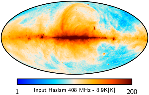
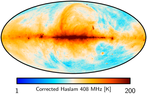
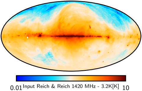
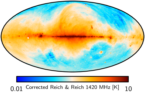
Figure 8: Comparison of the 408 (top) and 1420 (bottom) MHz low-frequency maps before (left) and after (right) offset corrections.

Next, in Fig. 8 we compare the pre- and post-correction 408 and 1420 MHz maps. The single most striking feature in this plot is a clear dipole extending from south to north in the 1420 MHz map. Converting the Cartesian dipole coefficients for the 1420 MHz map in Table 1 into spherical coordinates, we find that the best-fit dipole is $0.15\pm 0.03$K, pointing towards Galactic coordinates $(l,b)=(308^{\circ},-36^{\circ})\pm 14^{\circ}$. Interestingly, this direction is consistent with the Equatorial south pole, $(l,b)=(303^{\circ},-27^{\circ})$, possibly suggesting that the observed dipole might be interpreted effectively in terms of an declination dependent offset.

After offset corrections, one can still see hints of an east-west type dipole in both the 408 and 1420 MHz maps. It is not directly obvious whether this feature is physical or not, as the dipole X and Y dipole coefficients for these maps are quite large (as well as correlated), and if for instance the Y-dipole in the 408 MHz is shifted by only one standard deviation, from 0.7 to 2.1K, the visual impression becomes far more symmetric. On the other hand, it is worth noting that the low-frequency WMAP polarization maps shows a similar asymmetry (see, e.g., Fig. 4 in Bennett et al. 2013), due to the presence of strong synchrotron radiation near the Fan region.

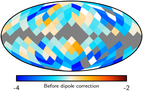
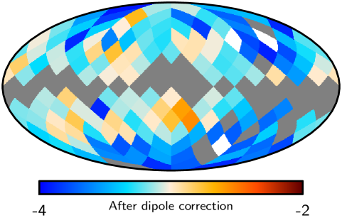
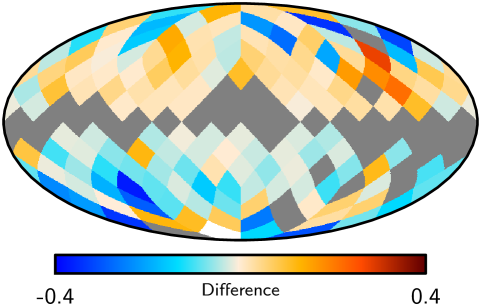
Figure 9: Estimates of the spectral index derived from the combination of the 408 and 1420 MHz maps using T–T plots, both before (top) and after (middle) applying the offset corrections. The bottom panel shows the difference. These differences show directly the magnitude of the bias in T–T plot based spectral indices due to spurious dipoles.

In Fig. 9 we compare the spectral index between the 408 and 1420 MHz maps before and after offset corrections, as estimated from the T–T plot distributions. Note that since monopoles do not change the index at all, these differences are all due to the dipole correction. Thus, the typical dipole-induced bias on the mean spectral index as computed over $N_{\textrm{side}}=4$ regions is $\pm 0.2$ for these maps.

Finally, we consider the stability of the derived results by comparing the results from the 17 and 14 band analyses, as presented in the top and bottom sections of Table 1. First, regarding the low-frequency 408 and 1420 MHz channels, we see that almost all deviations are smaller than $1\sigma$ when including 16% more sky area, with the biggest difference is seen for the 408 MHz monopole at $1.3\sigma$.

On the high frequency side, we see that the 353 GHz monopole of $315\pm 9\thinspace\mu\textrm{K}$ derived within the 17 band solution is in excellent agreement with HI cross-correlation result of $308\thinspace\mu\textrm{K}$ (Planck Coll. VII 2013). The 353 GHz dipoles shows larger variations at the $2\sigma$ level. Imposing an HI prior also on this component should prove useful for the 14-band analysis.

For the CMB-dominated frequencies, we see that the dipoles are overall in good agreement in terms of absolute numbers, despite the fact that the WMAP dipoles are forced to zero. This robustness gives added credibility to the derived Planck dipoles. On the other hand, it is also clear that the reported uncertainties are too small, as already seen in simulations.

Finally, we note relatively large differences in the monopole values for frequencies between 23 (K-band) and 94 GHz (W-band), both for WMAP and Planck. This may be linked to the relatively large K-band dipole of $16\pm 4\thinspace\mu\textrm{K}$ in the 17-band analysis; when forcing this value to be zero, the monopole at the same frequency increases from $-14$ to $27\thinspace\mu\textrm{K}$, and this must in turn be accommodated by increased monopoles at higher frequencies.

5 Summary and conclusions

One of the most difficult tasks in physical CMB component separation is the determination of absolute offsets, i.e., spurious monopoles and dipoles. Unless accounted for, such offsets may bias the estimation of spectral parameters significantly, and this can in turn lead to errors in the actual CMB map. Ideally, the optimal approach would be to fit the offsets and foreground model jointly, as for instance implemented by Gibbs sampling (Eriksen et al. 2008); however, if the data model contains a large number of spectral indices, say, one per square degree pixel, the system is often not sufficiently rigid to uniquely determine the optimal solution. The offsets are nearly degenerate with the effective zero-level of each foreground component, and the only feature that breaks this degeneracy is spatial variation in the spectral parameters.

In this paper, we have presented an alternative method for estimating spurious monopoles and dipoles in multi-frequency data sets. This method builds on a well-established methodology from the radio astronomy literature called T–T plots. The main advantages of this method over the Bayesian approach are that 1) it makes minimal assumptions about the nature of the signal components, 2) it is computationally cheap, and 3) it is trivial to tune the number of regions to the point that the degeneracy between the spectral indices and the offsets are broken. The latter can of course also be implemented within the Bayesian framework, at which point we expect the two methods to perform similarly. The main disadvantage of the current method is a relatively large systematic uncertainty when no signal component dominates, which for CMB purposes typically happens near the foreground minimum at 70 GHz. In the present paper, we have adopted a straight template-fit approach for these frequencies, but note that a true multi-component fit is certainly preferable. The most likely application for the current method is therefore to set the offsets at the foreground-dominated frequencies, which will then serve as an “anchor” for the Bayesian fit, effectively breaking the degeneracies between the offsets and the spectral parameters.

The main products presented in the paper are two different, but each internally consistent, sets of monopole and dipole coefficients. Overall, the two sets agree well with each other, except for a single common monopole extending from 23 to 94 GHz. This is largely due to the significant systematic uncertainty associated with the WMAP K-band and Planck 30 GHz offsets. We recommend that methods employing our offset values for subsequent analyses consider both sets for systematic uncertainty assessment.

An early version of the method presented in this paper was already adopted by the 2013 Planck release to determine the zero-levels for the physical component separation results, but only applied to the Planck frequencies between 30 and 353 GHz (Planck Coll. XII 2013). In this paper we have extended the total data set to also include the WMAP frequencies, the Planck 545 and 857 GHz frequencies, and the $100\thinspace\mu\textrm{m}$ SFD map. Overall, the results presented here are in good agreement with the earlier results, with a largest relative monopole difference of $2\thinspace\mu\textrm{K}$ for all channels between 30 and 217 GHz. The only significant outlier is the 353 GHz channel, for which we derive a value of $315\pm 9\thinspace\mu\textrm{K}$, whereas Planck Coll. XII (2013) obtained a value of $414\thinspace\mu\textrm{K}$. A third and fully independent estimate of this number was provided by Planck Coll. VII (2013) based on cross-correlation with HI observations, who reported a value of $308\pm 23\thinspace\mu\textrm{K}$, in excellent agreement with our result. Similarly, at 857 GHz Planck Coll. VII (2013) reports a value of $0.147\pm 0.0147\thinspace\textrm{MJy/sr}$ from HI measurements, which is to be compared with our fully internal estimate of $0.17\pm 0.03\thinspace\textrm{mK}$; for the 545 GHz the corresponding numbers are $0.107\pm 0.017$ to be compared with our value of $0.12\pm 0.01$. Other channels are also in good agreement. However, for the SFD 100$\thinspace\mu$m map, we note that the X-dipole has both a large value and a large uncertainty, suggesting a less constrained fit overall. This is not unexpected, as this particular channel is only coupled to the Planck 857 GHz map through a long frequency extrapolation. The offset values for this channel are clearly less robust than for the HFI channels, and its role is primarily to stabilize the 857 GHz results, rather than derive independent and robust offsets for the SFD map itself.

On the low-frequency side, the 408 MHz and 1420 MHz monopoles have already been subject of considerable discussion in the literature. Haslam et al. (1982) estimated that the zero-level uncertainty of the 408 MHz survey was $\pm 3\thinspace\textrm{K}$, with an additional multiplicative calibration of 10%. The corresponding data for the 1420 MHz survey are $\pm 0.5\thinspace\textrm{K}$ and 5% (Reich & Reich 1988). Lawson et al. (1987) used a comparison with a 404 MHz map to determine a uniform background for an assumed correct zero-level of $5.9\thinspace\textrm{K}$, which consists of the CMB monopole and an isotropic extra-galactic contribution from source counts. They also quote a zero-level correction of $-0.13\thinspace\textrm{K}$ for the 1420 MHz survey, where the uniform background is $2.8\thinspace\textrm{K}$. From a TT-plot analysis Reich & Reich (1988) found a $-2.1\thinspace\textrm{K}$ zero-level offset for the 408 MHz survey, when assuming that the zero-level at 1420 MHz is correct. Later, Reich et al. (2004) used an improved source-count correction, which results in a uniform background at 408 MHz of $5.4\pm 0.6\thinspace\textrm{K}$. The zero-level correction is $-2.7\thinspace\textrm{K}$ then. Tartari et al. (2008) used absolute brightness measurements at 600 MHz and 820 MHz and derived zero-level offsets of $-3.9\pm 0.6\thinspace\textrm{K}$ at 408 MHz and $-0.12\pm 0.14\thinspace\textrm{K}$ at 1420 MHz. All together these studies show that the zero-level of the 408 MHz survey is too low and requires corrections between $+2.1\thinspace\textrm{K}$ and $+3.9\thinspace\textrm{K}$, while the 1420 MHz survey requires corrections up to $+0.13\thinspace\textrm{K}$. All these studies assume that the remaining extended emission in the survey maps is of Galactic origin. Spectral index maps (Reich & Reich 1988; Lawson et al. 1987, e.g.,) do not contradict this assumption. However, the minima in the survey maps at 408 MHz and 1420 MHz, with the zero-level, isotropic source-count and CMB corrections by the Reich et al. (2004) values, are about $9.5\thinspace\textrm{K}$ and $0.4\thinspace\textrm{K}$ at 2$\degr$ angular resolution. This means that there is room for a Galactic contribution to a monopole and higher order components, but also for a larger isotropic extra-galactic component than calculated from source counts, as discussed in Sun & Reich (2010). Without any correction the survey minima are $12.2\thinspace\textrm{K}$ and $3.2\thinspace\textrm{K}$ at 2$\degr$ resolution, respectively, which constrain the monopole components when derived directly from the survey data. Recently, Bennett et al. (2013) used the same co-secant method as they applied to the WMAP CMB frequencies to derive a background value of $7.4\thinspace\textrm{K}$ at 408 MHz. Fornengo et al. (2014) used six surveys to model the Galactic synchrotron and thermal emission and found an isotropic background value, without CMB, of $11.8\pm 1.1\thinspace\textrm{K}$ at 408 MHz and $0.58\pm 0.025\thinspace\textrm{K}$ at 1420 MHz. They conclude that their results agree with the extra-galactic component from ARCADE 2 (Fixsen et al. 2011). Subramanian & Cowsik (2013) also modelled the Galactic disk and halo emission and showed that the simple co-secant method used to fit Galactic emission is the reason for the ARCADE 2 excess and that there is no need for an isotropic extra-galactic component beyond that from source counts. The currently deepest source count data by Vernstrom et al. (2014), which also include diffuse extra-galactic emission at 1.75 GHz, give a strong indication that the excessive temperature found by ARCADE 2 is not of extra-galactic origin. Our current monopole values of $8.9\pm 1.3\thinspace\textrm{K}$ for 408 MHz and $3.28\pm 0.02\thinspace\textrm{K}$ at 1420 MHz are in the possible range allowed by the survey data.

While the method presented in this paper is very general, and can deal with spurious monopole and dipoles of any origin, it is worth noting that by far the dominant source of dipole uncertainty in current CMB maps comes from estimating the solar CMB dipole. For instance, even small calibration uncertainties can lead to a significant uncertainties in the recovered dipole. However, this uncertainty is perfectly correlated between channels within a given experiment, and it is therefore possible to impose the prior that the corrections should be identical across frequencies.

Finally, we conclude with two important caveats. First and foremost, it is important to realize that while the method presented here is extremely efficient at establishing relative offsets between channels (which by far is the most important problem for most component separation algorithms), it requires both high signal-to-noise observations and significant spatial spectral variations across the sky to determine absolute offsets. With the data sets studied in this paper, it appears that these criteria hold for both the low-frequency 408 and 1420 MHz maps and the high-frequency channels above 100 GHz, but not for the intermediate CMB channels between 23 and 94 GHz. Again, as shown in Section 3 the systematic uncertainty on the WMAP K-band offsets is large. More conservatively, we caution against adopting any of the derived offsets for frequencies between 23 and 44 GHz without further cross-checks because of the presence of multiple significant foreground components (i.e., synchrotron, free-free and AME). Instead a full parametric fit is should be used for these channels. Second, we emphasize that accurate uncertainty estimation is difficult, because the dominant sources of uncertainties are generally systematic in nature. In the present paper, we have adopted an internal bootstrap approach, which is able to capture some, but not all, of these uncertainties. For more realistic systematic uncertainty assessment, we recommend propagating both offset sets provided in this paper through subsequent analyses.