The in-plane gradient magnetic field induced vortex lattices in spin-orbit coupled Bose-Einstein condensations

Abstract

We consider the ground-state properties of the two-component spin-orbit coupled ultracold bosons subject to a rotationally symmetric in-plane gradient magnetic field. In the non-interacting case, the ground state supports giant-vortices carrying large angular momenta without rotating the trap. The vorticity is highly tunable by varying the amplitudes and orientations of the magnetic field. Interactions drive the system from a giant-vortex state to various configurations of vortex lattice states along a ring. Vortices exhibit ellipse-shaped envelops with the major and minor axes determined by the spin-orbit coupling and healing lengths, respectively. Phase diagrams of vortex lattice configurations are constructed and their stabilities are analyzed.

I introduction

Spin-orbit (SO) coupling plays an important role in contemporary condensed matter physics, which is linked with many important effects ranging from atomic structures, spintronics, to topological insulators zutic2004 ; Hasan2010 ; Qi2011 . It also provides a new opportunity to search for novel states with ultracold atom gases which cannot be easily realized in condensed matter systems. In usual bosonic systems, the ground state condensate wavefunctions are positive-definite known as the “no-node” theorem feynman1972 ; wu2009 . However, the appearance of SO coupling invalidates this theorem wu2011 . The ground state configurations of SO coupled Bose-Einstein condensations (BEC) have been extensively investigated and a rich structure exotic phases are obtained including the ferromagnetic and spin spiral condensations wu2011 ; stanescu2008 ; wang2010 ; ho2011 , spin textures of the skyrmion type wu2011 ; hu2012 ; sinha2011 ; li2012 ; kawakami2012 , and quantum quasi-crystals gopalakrishnan2013 , etc. On the experiment side, since the pioneering work in the NIST group lin2009 , it has received a great deal of attention, and various further progresses have been achieved zhang2012v1 ; wang2012 ; cheuk2012 ; qu2013 ; olson2014 . Searching for novel quantum phases in this highly tunable system is still an on-going work both theoretically and practically wilson2013 ; achilleos2013 ; kartashov2013 ; ozawa2013 ; deng2012 ; zhang2012 ; lobanov2014 ; luo2014 , which has been reviewed in zhou2013 ; dalibard2011 ; zhai2014 ; galistki2013 ; goldman2013 .

On the other hand, effective gradient magnetic fields have been studied in various neutral atomic systems recently. For instance, it has been shown in Ref. anderson2013 ; xu2013 that SO coupling can be simulated by applying a sequence of gradient magnetic field pulses without involving complex atom-laser coupling. In optical lattices, theoretic and experimental progresses show that SO coupling and spin Hall physics can be implemented without spin-flip process by employing gradient magnetic field kennedy2013 ; aidelsburger2013 . This represents the cornerstone of exploring rich many-body physics using neutral ultracold atoms. Additionally, introducing gradient magnetic fields has also been employed to create various topological defects including Dirac monopoles pietila2009 and knot solitons kawaguchi2008 . It would be very attractive to investigate the exotic physics by combining both SO coupling and the gradient magnetic field together in ultracold quantum gases.

In this work, we consider the SO coupled BECs subject to an in-plane gradient magnetic field in a $2$D geometry. Our calculation shows that this system support a variety of interesting phases. The main features are summarized as follows. First, the single-particle ground states exhibit giant vortex states carrying large angular momenta. It is very different from the usual fast-rotating BEC system, in which the giant vortex state appears only as meta-stable states schweikhard2004 ; mueller2002 . Second, increasing the interaction strength causes the phase transition into the vortex lattice state along a ring plus a giant core. The corresponding distribution in momentum space changes from a symmetric structure at small interaction strengths to an asymmetric one as the interaction becomes strong. Finally, the size of a single vortex is determined by two different length scales, namely, the SO coupling strength together with the healing length. Therefore, the vortex exhibits an ellipse-shaped envelope with the principle axes determined by these two scales. This is different from the usual vortex in rotating BECs fetter2009 ; zhou2011 ; xu2011 ; radic2011 ; aftalion2013 ; fetter2014 , where an axial symmetric density profile is always favored.

The rest of this article is organized as follows. In Sect. II, the model Hamiltonian is introduced. The single particle wavefunctions are described in Sect. III. The phase transitions among different vortex lattice configurations are investigated in Sect. IV. The possible experimental realizations are discussed in Sect. V. Conclusions are presented in Sect. VI.

II The model Hamiltonian

We consider a quasi-$2$D SO coupled BEC subject to a spatially dependent magnetic field with the following Hamiltonian as

$$H=\int d\vec{r}^{2} \hat{\psi}(\vec{r})^{{\dagger}}\Big{\{}\frac{\vec{p}^{2}}{2m}+\Lambda r\left(\cos\theta\hat{r}+\sin\theta\hat{\varphi}\right)\cdot\vec{\sigma}$$ (1)

$$+ \frac{1}{2}m\omega^{2}r^{2}\Big{\}}\hat{\psi}(\vec{r})+H_{soc}+H_{int},$$

where $\hat{r}=\vec{r}/r$ with $\vec{r}=(x,y)$; $\vec{\sigma}=(\sigma_{x},\sigma_{y})$ are the usual Pauli matrices; $m$ is the atom mass; $\omega$ is the trapping frequency; $\Lambda$ is the strength of the magnetic field, and $\theta$ denotes the relative angle between the magnetic field and the radial direction $\hat{r}$. Physically, this quasi-2D system can be implemented by imposing a highly anisotropic harmonic trap potential $V_{H}=\frac{1}{2}m(\omega^{2}r^{2}+\omega^{2}_{z}z^{2})$. When $\omega_{z}\gg\omega$, atoms are mostly confined in the $xy$-plane, and the wavefunction along $z$ axis is determined as a harmonic ground state with the characteristic length $a_{z}=\sqrt{\hbar/(m\omega_{z})}$.

For simplicity, the SO coupling employed below has the following symmetric form as

$$H_{soc} = \int d\vec{r}^{2}\hat{\psi}(\vec{r})^{{\dagger}}\Big{[}\frac{\lambda}{m}(p_{x}\sigma_{x}+p_{y}\sigma_{y})\Big{]}\hat{\psi}(\vec{r})$$

with $\lambda$ the SO coupling strength. We note that due to this term, the magnetic fields which couples to spin can be employed as a useful method to control the orbit degree of freedom of the cloud. The interaction energy is written as

$$H_{int}=\frac{g_{2D}}{2}\int d\vec{r}^{2}\hat{\psi}(\vec{r})^{{\dagger}}\hat{\psi}(\vec{r})^{{\dagger}}\hat{\psi}(\vec{r})\hat{\psi}(\vec{r}).$$ (2)

Here the contact interaction between atoms in bulk is $g=4\pi\hbar^{2}a_{s}/m$, where $a_{s}$ is the scattering length. For the quasi-2D geometry that we focus on, the effective interaction strength is modified as $g_{2D}=g_{3D}/(\sqrt{2\pi}a_{z})$.

III single-particle properties

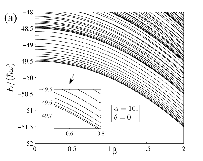
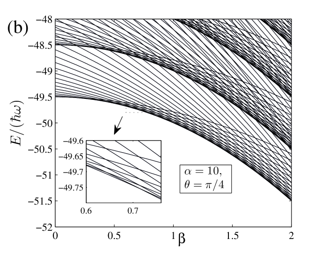
Figure 1: The single-particle dispersion of the Hamiltonian Eq. (3) with lower energy branch as a function of the reduced magnetic fields $\beta$ for fixed $\alpha=10$ and different values of $\theta=0$ (a), and $\frac{1}{4}\pi$ (b). The inset in (b) shows that the ground states crossing for certain values of $\beta$ at $\theta=\pi/4\neq 0$, while there is no crossing in (a) at $\theta=0$.

The physics of Eq. 1 can be illustrated by considering the single-particle properties first. After introducing the characteristic length scale of the confining trap $l_{T}=\sqrt{\hbar/m\omega}$, the dimensionless Hamiltonian is rewritten as

$$\frac{H_{0}}{\hbar\omega}=\int d\vec{\rho}^{2} \hat{\phi}(\vec{\rho})^{{\dagger}}\Big{\{}-\frac{\vec{\nabla}^{2}}{2}+\beta\rho\left(\cos\theta\hat{r}+\sin\theta\hat{\varphi}\right)\cdot\vec{\sigma}$$ (3)

$$+ \alpha\vec{k}\cdot\vec{\sigma}+\frac{1}{2}\rho^{2}\Big{\}}\hat{\phi}(\vec{\rho}),$$

where $\alpha=\lambda/(m\omega l_{T})$ and $\beta=\Lambda l_{T}/(\hbar\omega)$ are the dimensionless SOC and magnetic field strengths, respectively; the normalized condensates wave-function is defined as

$$\phi(\vec{\rho})=\frac{l_{T}}{\sqrt{N}}\Psi(\vec{r}=l_{T}\vec{\rho})$$

with $N$ the total number of atoms;

Since the total angular momentum $\hbar j_{z}=\hbar l_{z}+\frac{\hbar}{2}\sigma_{z}$ is conserved for this typical Hamiltonian, we can use it to label the single-particle states. If the magnetic field along the radial direction, i.e., $\theta=l\pi$, the Hamiltonian also supports a generalized parity symmetry described by $i\sigma_{y}P_{x}$, namely

$$[H_{0},i\sigma_{y}P_{x}]=0,$$ (4)

with $P_{x}$ the reflection operation about the $y$-axis satisfying $P_{x}:(x,y)\rightarrow(-x,y)$. Therefore for given eigenstates $\phi_{m}=[f(\rho)e^{im\varphi},g(\rho)e^{i(m+1)\varphi}]^{T}$ with $j_{z}=(m+1/2)$, the above symmetry indicates that these two states $\{\phi_{m},(i\sigma_{y}P_{x})\phi_{m}\}$ are degenerate for $H_{0}(\theta=l\pi)$. This symmetry is broken when $\theta\neq l\pi$.

Due to the coupling between the real space magnetic field and momentum space SO coupling, the single particle ground states exhibit interesting properties at large values of $\alpha$ and $\beta$. In momentum space, the low energy state moves to a circle with the radius determined by $\alpha$. The momentum space single-particle eigenstates break into two bands $\psi^{\pm}(\vec{k})$ with the corresponding eigenvalues $E^{\pm}_{\vec{k}}/(\hbar\omega)=\frac{1}{2}(|\vec{k}|^{2}\pm 2\alpha|\vec{k}|)$ and eigenstates $\frac{1}{\sqrt{2}}[1,\pm e^{i\theta_{k}}]^{T}$, respectively. For the lower band which we focus on, the spin orientation is $\langle\vec{\sigma}\rangle=(-\cos\theta_{\vec{k}},-\sin\theta_{\vec{k}})$, which is anti-parallel to $\vec{k}$. On the other hand, in the real space, for a large value of $\beta$, the potential energy in real space is minimized around the circle with the the radius $r/l_{T}=\beta$ with a spatial dependent spin polarization. Therefore around this space circle, the local wavevector at a position $\vec{r}$ is aligned along the direction of the local magnetic field to minimize the energy. The projection of the local wavevector along the tangent direction of the ring gives rise to the circulation, and thus the ground state carries large angular momentum $m$ which is estimated as

$$m\simeq 2\pi\beta\sin\theta/(2\pi/\alpha)=\alpha\beta\sin\theta.$$ (5)

Therefore, by varying the angle $\theta$, a series of ground states are obtained with their angular momentum ranging from $0$ to $\alpha\beta\gg 1$. This is very different from the usual method to generate giant vortex, where fast rotating the trap is needed fetter2009 .

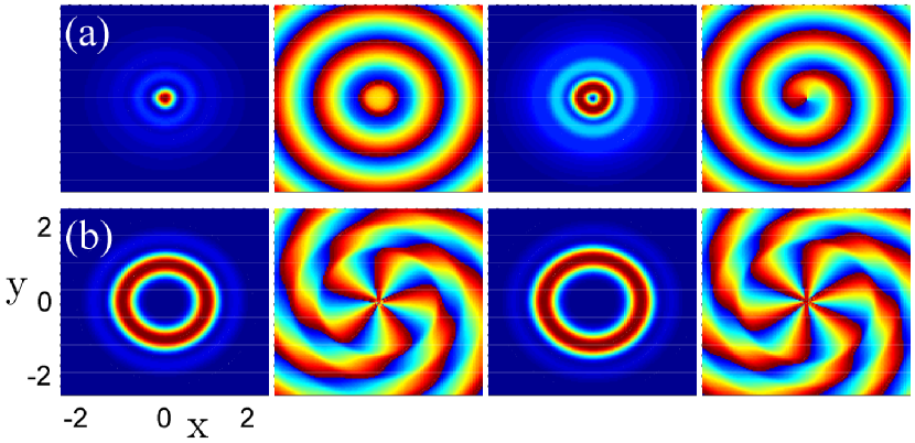
Figure 2: The density and phase profiles of the single-particle ground states for fixed $\alpha=6$, $\beta=1$, and different $\theta=\frac{1}{40}\pi$ (a), $\frac{2}{5}\pi$ (b). From left to right: the density and phase profiles for spin-up and spin-down components, respectively.

For $\beta\gg 1$, the low energy wavefunctions mainly distribute around the circle $\rho=\beta$. As shown in Appendix A, the approximated wavefunctions for the lowest band ($n=1$) is written as

$$\phi_{n=1,j_{z}}(\rho,\varphi) \simeq \frac{1}{2\pi^{\frac{3}{4}}\rho^{\frac{1}{2}}}e^{-\frac{(\rho-\beta)^{2}}{2}}e^{i\rho\alpha\cos\theta}$$ (8)

$$\times \left[\begin{array}[]{c}e^{i[m\varphi-\frac{\theta}{2}]}\\ -e^{i[(m+1)\varphi+\frac{\theta}{2}]}\end{array}\right],$$

where $\varphi$ is the azimuthal angle. The corresponding energy dispersion is approximated as

$$E_{n,j_{z}}\approx n+\frac{1-\alpha^{2}-\beta^{2}}{2}+\frac{(j_{z}-\alpha\beta\sin\theta)^{2}}{2(\alpha^{2}\cos^{2}\theta+\beta^{2})}.$$ (9)

For given values of $\alpha$ and $\beta$, $E_{n,j_{z}}$ is minimized at $j_{z}\simeq\alpha\beta\sin\theta$, which is consistent with the above discussion. In the case of $\theta=l\pi$, two states with $m=l$ and $-(l+1)$ are degenerated due to the symmetry defined in Eq. 4. Interestingly, Eq. 9 also indicates that for integer $\alpha\beta\sin\theta=l$, an approximate degeneracy occurs for $m=l$ and $l-1$.

Fig. 1 shows the single-particle dispersion of different angular momentum eigenstates along with the radius $\beta$ for different values of $\theta$. For $\theta=0$, the dispersion with different $j_{z}$ never cross each other Fig. 1 (1a). The values of $j_{z}$ for the ground state are always $j_{z}=\frac{1}{2}$ or $-\frac{1}{2}$ due to the symmetry Eq. 4. When $\theta=\pi/4\neq 0$, the spectra cross at certain parameter values, and the ground-state can be degenerate even without additional symmetries as shown in Fig. 1 (1b), which is consistent with above discussions. For $\beta\gg 1$, the probability density of the ground state single particle wavefunction mainly distributes around a ring with $\rho=\beta$. Interestingly, the phase distribution exhibits the typical Archimedean spirals with the equal-phase line satisfying $\rho\sim m\varphi$ (or $\rho\sim(m+1)\varphi$) (see Fig. 2 for details).

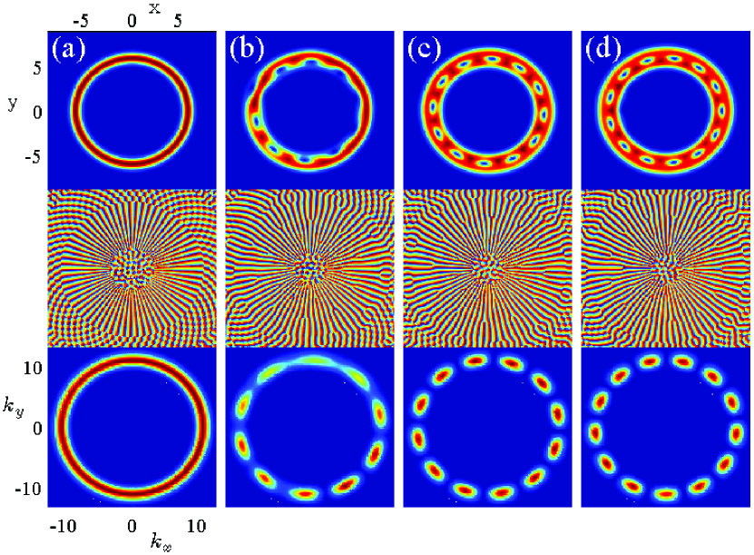
Figure 3: The profiles of the condensate wavefunctions of the spin-up component for $\alpha=11$, $\beta=6$, and $\theta=\frac{\pi}{2}$. The interaction parameters are $g=15$ ($a$), 35 ($b$), 75 ($c$), and 100 ($d$), respectively. We note that (c) and (d) exhibit similar profiles but with different $q$. From top to bottom: the density and phase profiles in real space, and the momentum distributions which mainly are located around the circle $|k|=\alpha$.

IV Phase transitions induced by interaction

In this section, we consider the interaction effect which will couple single-particle eigenstates with different values of $j_{z}$. It is interesting to consider the possible vortex configurations in various parameter regimes, which has been widely considered in the case of the fast rotating BECs.

If the dimensionless interaction parameter $g=g_{2D}N/(\hbar\omega l_{T}^{2})$ is small, it is expected that the ground state still remains in a giant-vortex state, which is similar to the non-interacting case. The envelope of the variational wave-function is approximated as

$$\phi_{j_{z}}(\rho,\varphi)\sim\frac{1}{2\pi^{\frac{3}{4}}\sqrt{\sigma\rho}}e^{-\frac{(\rho-\beta)^{2}}{2\sigma^{2}}}e^{i\rho\alpha\cos\theta}\left[\begin{array}[]{c}e^{i[m\varphi-\frac{\theta}{2}]}\\ -e^{i[(m+1)\varphi+\frac{\theta}{2}]}\end{array}\right]$$ (12)

with $\sigma$ the radial width of the condensates. Around a thin ring inside the cloud with the radius $\rho$, in order to maintain the overall phase factor $e^{im\varphi}$, the magnitude of the local momentum along the azimuth direction is determined by $k_{\varphi}=m/\rho$. Depending on the width $\sigma$ of the cloud, the linewidth of $k_{\varphi}$ is proportional to $\delta k_{\varphi}=m\sigma/\beta^{2}$. In momentum space, this leads to the expansion of the distribution around the ring with $|k|=\alpha$. The increasing of the kinetic energy mainly comes from the term $\hat{E}_{\varphi}=(j_{z}/\rho-\alpha\sin\theta)^{2}/2$, which is estimated as $\langle\hat{E}_{\varphi}\rangle_{j_{z}}$. Details derivation of various energy contributions can be found in Appendix B.

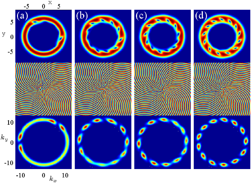
Figure 4: Ground state profiles of the condensates for $\alpha=11$, $\beta=6$, $\theta=\pi/3$ with different interaction $g=85$(a), $105$(b), $125$(c), and $145$(d) respectively. From top to bottom: density and phase profiles of the spin-up component, momentum distribution in the lower band along the circle $|k|=\alpha$. The orientation of the ellipse-shaped vortices is determined by $\theta$. See text for details.

Increasing the interaction strength $g$ expands the cloud and leads to larger width $\sigma$ and $\delta k_{\varphi}$, which makes the above variational state energetically unfavorable. In order to minimize the total energy, the condensates tend to involve additional vortices such that the local momentum mainly distributes around the circle $|k|=\alpha$ with smaller $\delta k_{\varphi}$ . Fig. (3) and (4) show the typical ground-state configurations for selected parameters. The phase accumulations around the inwards and outwards boundaries of the cloud are $2\pi m_{+}$ and $2\pi m_{-}$ respectively. Therefore, there are $q=m_{+}-m_{-}$ vortices involved and distributed symmetrically inside the condensates. Between two nearest vortices, the local wavefunction can be approximately determined as a plane-wave state. Therefore, their corresponding distribution in momentum space is also composed of $q$ peaks located symmetrically around the circle $|k|=\alpha$.

As further increase of the interaction strength, the condensates break into more pieces by involving more vortices. The number of the vortices is qualitatively determined by the competition of the azimuthal kinetic energy and the kinetic energy introduced by the vortices. Specifically, if $q$ vortices locate in the middle of the cloud around the circle $\rho_{0}\simeq\beta$, then for the inwards part of the condensates with $\rho<\rho_{0}$, the mean value of the angular momentum can be approximated as $j_{z,-}\approx j_{z}-q/2$, while for the regime with $\rho>\rho_{0}$, we have $j_{z,+}\approx j_{z}+q/2$. The corresponding kinetic energy along the azimuthal direction is modified as

$$\langle\hat{E}_{\varphi}\rangle = \langle\hat{E}_{\varphi}\rangle_{j_{z}}+\frac{q}{2\beta^{2}}(\frac{q}{4}-\frac{\sigma\alpha\sin\theta}{\sqrt{\pi}}).$$ (13)

This indicates that, to make the vortex-lattice state favorable, we must have $(\frac{q}{4}-\frac{\sigma\alpha\sin\theta}{\sqrt{\pi}})<0$. In the limit case with $\theta=0$, this condition is always violated. Therefore, the ground state remains to be an eigenstate of $j_{z}$ with $j_{z}=\pm\frac{1}{2}$ even for large interaction strength.

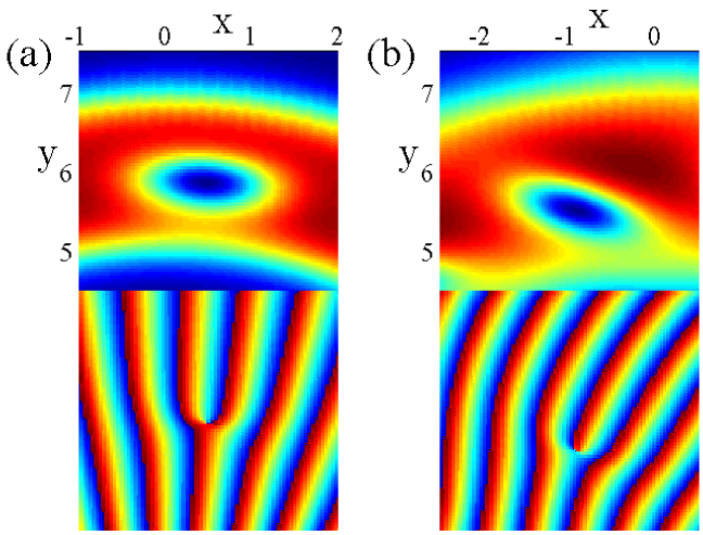
Figure 5: Enlarged density and phase profiles around single vortex. The two figures (a) and (b) are the corresponding parts adapted from Fig. (3c) and (4d) respectively.

We note the vortices display an ellipse-like shape with two main axis, as shown in Fig. 5. The phase profile is twisted, and the constant phase front exhibits a dislocation around vortex cores. Along the direction of local wavevector $\vec{k}$, the vortex density profile is determined by the length scale $2\pi l_{T}/\alpha$. While perpendicular to the direction of local $\vec{k}$, the vortex profile is dominated by the healing length $\xi$ due to interaction. Therefore, the vortex density distribution is determined by two different length scales in mutually orthogonal directions, which results in ellipse-shaped vortices. Changing the interaction strength and SO coupling alerts the ratio of the two length scales, thus changes the eccentricity of the ellipses. Additionally, changing the angle $\theta$ also changes the direction of local magnetic fields, and thus modifies the orientation of the vortices, as shown in Fig. 3 and Fig. 4.

On the other hand, the introduction of vortices lead to the increase of kinetic energy due to the modification of the density profile. This can be estimated as $0.19q/(\beta\sigma\alpha\xi)$, where $\xi=1/\sqrt{2gn_{0}}$ is the dimensionless healing length with $n_{0}$ the bulk density of the clouds. The total energy changing due to the presence of the vortices can be written as

$$\Delta E=\frac{q}{2\beta^{2}}(\frac{q}{4}-\frac{\sigma\alpha\sin\theta}{\sqrt{\pi}})+\frac{0.19q}{\beta\sigma\alpha\xi}.$$ (14)

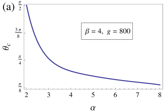
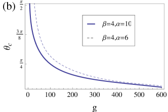
Figure 6: (a) Critical angle $\theta_{c}$ as a function of SO coupling strength $\alpha$ for fixed values of $\beta=4$ and $g=800$. (b) $\theta_{c}$ decreases as the increase of interaction parameter $g$ for fixed $\alpha=10$, $6$, and $\beta=4$.

Several interesting features can be extracted from Eq. 14. For fixed parameters $g$, $\alpha$, and $\beta$, there always exists a critical $\theta_{c}$ such that $\Delta E=0$ is satisfied. When $\theta<\theta_{c}$, then $\Delta E>0$, which indicates that a giant-vortex ground state is always favored. As increasing $\alpha$, $\theta_{c}$ satisfying $\Delta E=0$ becomes smaller. At $\theta>\theta_{c}$, the ground state exhibits a lattice-type structure along the ring with a giant vortex core. The values of $q$ is determined by minimizing $\Delta E$ with respect to $g$, $\alpha$, and $\beta$, respectively. Fig. (6) shows $\theta_{c}$ as a function of SO strength $\alpha$ at which the transition from a giant-vortex state to a vortex-lattice state occurs. When $\alpha$ is small, a giant-vortex state is favored for all values of $\theta$. As $\alpha$ increases, $\theta_{c}$ drops quickly initially and decreases much slower when $\alpha$ becomes large as shown in Fig. (6) (a). In Fig. (6) (b), it shows that as increasing the interaction $g$, it is becomes easier to drive the system into the vortex lattice state.

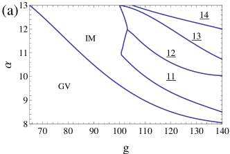
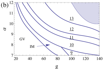
Figure 7: Phase diagram in the $\alpha-g$ plane for $\beta=6$ with different $\theta=\pi/3$ ((a)) and $\pi/2$ ((b)). The number $\underline{M}$ means that the condensates support a vortex-lattice-type ground state with $M$ momentum peaks along the circle $|k|=\alpha$. The regime with shadow in (b) indicates the ground state shows multi-layer structure as increasing the interaction strength. Other phases are defined as follows: GV(giant-vortex state),IM (intermediate regime).

Fig. (7) shows the phase diagram in the $\alpha-g$ plane for a fixed $\beta=6$ for different values of $\theta$. For a fixed $\alpha$ and at small values of $g$, the system remains to be a giant-vortex state until $g$ reaches its critical value $g_{c}$. When $g>g_{c}$, the system enters into an intermediate regime in which vortices start to enter into the condensates from boundaries. The momentum distribution also breaks into several disconnected segments. More single quantum vortices are generated in the condensates as further increasing the interaction strength. The vortices distribute symmetrically along the ring and separate the condensates into pieces. Between two neighboring vortices, the condensates are approximated by local plane-wave states. The momentum distribution composes of multi-peaks symmetrically located around the circle $|k|=\alpha$. Increasing $g$ also increases the number of the single quantum $M$ inside the condensates, hence increases the number of peaks in momentum space. For a smaller value $\theta=\pi/3$, the critical $g_{c}$ is increased, which means that stronger interactions are needed to drive the system into the vortex-lattice states. Interestingly, the intermediate regime is also greatly enlarged. This is consistent with the limit case $\theta=0$, where the system remains to be a giant-vortex state even in the case of large interaction strength.

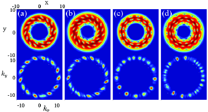
Figure 8: Density and momentum distributions about the ground states of the condensates for $\theta=\pi/3$ with $g=400$((a)), $1000$((b)), and $\theta=\pi/2$ with $g=400$((c)), $1000$((d)). Other parameters are the same with figure (4). We note that since the two spin components share almost the same profiles, only the densities of the spin-up component are shown for simplicity.

More ellipse-shaped vortices are formed as further increasing the interaction strength, which are self-organized into a multiple layered ring structure, as shown in Fig.(8). Around each ring, vortices distributed symmetrically. The number of the vortices between different layers can be not equal due to their different radius. Therefore the distribution in momentum space becomes asymmetric, and exhibits complex multi-peak structures around the circle $|k|=\alpha$.

V Experimental consideration

The Hamiltonian Eq. 1 considered above can be dynamically generated on behalf of a series of gradient magnetic pulses anderson2013 ; xu2013 . Starting with the typical single-particle Hamiltonian $H_{s}=\frac{p^{2}}{2m}+\frac{1}{2}m\omega^{2}r^{2}$, in the first time step, we employ a pair of magnetic pulses $U_{1}$ and $U_{1}^{\dagger}$, defined as as

$$U_{1}=e^{i\lambda(x\sigma_{x}+y\sigma_{y})/\hbar},$$ (15)

at time $t=2n\tau$, $(2n+1)\tau$ respectively. Secondly, a typical effective gradient coupling,

$$\Lambda[(x\cos\theta-y\sin\theta)\sigma_{x}+(y\cos\theta+x\sin\theta)\sigma_{y}],$$ (16)

is applied during the whole time duration $[(2n+1)\tau,2(n+1)\tau]$. Combining these two time steps, an effective dynamical evolution $U=e^{-iH_{0}\tau}$, which implements the desired dynamics. In practice, the gradient magnetic pulse in the first cycle can be simulated with quadrupole fields as $\vec{B}=(x,y,-2z)$. When the condensates is strongly confined in the $xy$ plane, the influence of the nonzero gradient along $z$-axis can be neglected. The effective gradient coupling in the second cycle can be implemented with the help of atom-laser coupling. For instance, a standard two-set Raman beams with blue-detuning liu2014 can realize an effective coupling

$$\Omega[\sin(\vec{k}_{1}\cdot\vec{r})\sigma_{x}+\sin(\vec{k}_{2}\cdot\vec{r})\sigma_{y}],$$ (17)

where the wavevectors $\vec{k}_{1}$ and $\vec{k}_{2}$ in the $xy$ plane can be chosen as $\vec{k}_{1}=k(\cos\theta,-\sin\theta)$ and $\vec{k}_{2}=k(\sin\theta,\cos\theta)$. When $2\pi/k$ is much larger than the trap length $l_{T}$, the required effective coupling is approximately obtained. Finally, the phases discussed in the context can be detected by monitoring their corresponding density and momentum distributions using the setup of time of flight.

VI Concluding remarks

To summarize, we have discussed the ground state phase diagram of SO coupled BECs subject to gradient magnetic fields. Theoretical and numerical analyses indicate that the system supports various interesting vortex physics, including the single-particle giant-vortex states with tunable vorticity, multiple layered vortex-lattice-ring states, and the ellipse-shaped vortex profiles. Therefore, the combination of SO coupling and the gradient magnetic fields provides a powerful method to engineer various vortex states without rotating the trap. We hope our work will stimulate further research of searching for various novel states in SO coupled bosons subject to effective gradient magnetic fields.

VII Acknowledgement

X.F. Z., Z.W. Z., and G.C. G. acknowledge the support by NSFC (Grant Nos. 11004186, 11474266,11174270), National Basic Research Program of China (Grants No. 2011CB921204 and No. 2011CBA00200). C. W. is supported by the NSF DMR-1410375 and AFOSR FA9550-14-1-0168, and also acknowledges the support from the National Natural Science Foundation of China (11328403).

Appendix A Single particle eigenstates for large $\beta$

We start with the dimensionless Hamiltonian

$$\frac{H_{0}}{\hbar\omega}=\int d\vec{\rho}^{2}\hat{\phi}(\vec{\rho})^{{\dagger}}\Big{\{}-\frac{\vec{\nabla}^{2}}{2}+\beta\rho\left(\cos\theta\hat{r}+\sin\theta\hat{\varphi}\right)\cdot\vec{\sigma}+\alpha\vec{k}\cdot\vec{\sigma}+\frac{1}{2}\rho^{2}\Big{\}}\hat{\phi}(\vec{\rho}).$$ (18)

Since the total angular momentum is conserved, the single particle eigenstates can be written as $\phi_{m}=[f(\rho)e^{im\varphi},g(\rho)e^{i(m+1)\varphi}]^{T}$ with $j_{z}=(m+1/2)$. Substitute this wavefunction into their corresponding Schrödinger equations, we obtain

$$\left\{\frac{\hat{p}^{2}_{\rho}}{2}+\frac{j_{z}^{2}}{2\rho^{2}}+\frac{(\rho\sigma_{x}-\beta)^{2}}{2}-\alpha[(\hat{p}_{\rho}\cos\theta+\frac{j_{z}}{\rho}\sin\theta)\sigma_{x}\right.$$ (23)

$$\left.+(\frac{j_{z}}{\rho}\cos\theta-\hat{p}_{\rho}\sin\theta)\sigma_{y}]+\frac{j_{z}\sigma_{z}}{2\rho^{2}}\right\}\left[\begin{array}[]{c}\tilde{f}(\rho)\\ \tilde{g}(\rho)\end{array}\right]=E\left[\begin{array}[]{c}\tilde{f}(\rho)\\ \tilde{g}(\rho)\end{array}\right],$$

where $\tilde{f}(\rho)=f(\rho)e^{i\theta/2}$, $\tilde{g}(\rho)=g(\rho)e^{-i\theta/2}$, $\hat{p}_{\rho}=-i(\frac{\partial}{\partial\rho}+\frac{1}{2\rho})$ is the momentum operator along the radical direction. For large $\beta\gg 1$, these functions mainly distribute around the circle $\rho=\beta$ in the plane, so we consider the superposition $F^{\pm}(\rho)=\frac{1}{2}[\tilde{f}(\rho)\pm\tilde{g}(\rho)])$, which satisfies the following approximated equations as

$$\left(\frac{\hat{p}^{2}_{\rho}}{2}\mp\alpha\cos\theta\hat{p}_{\rho}+\frac{j_{z}^{2}}{2\rho^{2}}\mp\alpha\sin\theta\frac{j_{z}}{\rho}+\frac{\rho^{2}}{2}\mp\beta\rho\right)F^{\pm}(\rho)$$

$$\pm i\alpha\left(\hat{p}_{\rho}\sin\theta-\frac{j_{z}}{\rho}\cos\theta\right)F^{\mp}(\rho)=E_{j_{z}}F^{\pm}(\rho).$$

The above equation indicates that to minimize the kinetic energy, we need $\langle\vec{p}_{\rho}\rangle\simeq\alpha\cos\theta$. Around $\rho=\beta$, we have the approximated solutions as $F^{\pm}(\rho)\sim H_{n}(\rho\pm\beta)e^{-(\rho\pm\beta)^{2}/2}e^{\pm i\alpha\cos\theta\rho}$ with $H_{n}(r)$ the usual $n$-th Hermite polynomial. Therefore, $F^{+}$ is negligible since we always have $\rho>0$. The solution now can be written as $\tilde{f}(\rho)\simeq\tilde{g}(\rho)\propto H_{n}(\rho-\beta)e^{-(\rho-\beta)^{2}/2}e^{i\alpha\cos\theta\rho}$. So we obtain the approximated wavefunctions for the lowest band ($n=1$) as

$$\phi_{n=1,j_{z}}\simeq\frac{1}{(2\pi)^{\frac{3}{4}}\rho^{\frac{1}{2}}}e^{-\frac{(\rho-\beta)^{2}}{2}}e^{i\rho\alpha\cos\theta}\left[\begin{array}[]{c}e^{i[m\varphi-\frac{\theta}{2}]}\\ -e^{i[(m+1)\varphi+\frac{\theta}{2}]}\end{array}\right].$$ (26)

The dispersion is estimated as

$$E_{n,j_{z}}=n+\frac{1-\alpha^{2}-\beta^{2}}{2}+\frac{(j_{z}-\alpha\beta\sin\theta)^{2}}{2(\alpha^{2}\cos^{2}\theta+\beta^{2})},$$ (27)

which is minimized when $j_{z}\simeq\alpha\beta\sin\theta$, so for the kinetic term along the tangential direction $\hat{E}_{\varphi}=(\frac{j_{z}}{\rho}-\alpha\sin\theta)^{2}/2$.

Appendix B Energy estimation of vortix lattice states around the ring

For weak interaction, the condensates expands along the radial direction as the parameter $g$ is increased. When $g$ is large enough, to lower the kinetic energy, the system tends to involve vortices located around a ring inside the condensates, which separate the wavefunction into two parts. Inside the vortex-ring, the wavefunction for the spin-up component is approximated as a giant vortex with the phase factor $e^{i2\pi m_{-}\phi}$, while outside the ring, the mean angular momentum carried by single particle is approximated as $m_{+}\hbar$. The difference $q=m_{+}-m_{-}$ represents the vortex number inside the condensates. Therefore the variational ground-state can be approximated as follows

$$\phi(\rho,\phi)=\left\{\begin{array}[]{c}\phi_{j_{z}-q/2}(\rho,\phi)\mbox{ when }\rho\in(0,\beta),\\ \phi_{j_{z}+q/2}(\rho,\phi)\mbox{ when }\rho\in(\beta,\infty).\end{array}\right.$$ (30)

We also assumes that around the circle $\rho=\beta$, vortices are involved and self-organized to compensate the phase mismatch so that the the whole wavefunction is well-defined.

The increase of the kinetic energy mainly comes from the term $\hat{E}_{\varphi}=(\frac{j_{z}}{\rho}-\alpha\sin\theta)^{2}/2$. For ground state without lattices, the energy is estimated and denoted as

$$\langle\hat{E}_{\varphi}\rangle_{j_{z}}=\int^{\infty}_{0}d\rho\int^{2\pi}_{0}d\varphi\rho\phi^{{\dagger}}_{j_{z}}\frac{(j_{z}/\rho-\alpha\sin\theta)^{2}}{2}\phi_{j_{z}},$$ (31)

where we use $\langle\rangle_{j_{z}}$ to denote the mean values over the trivial variational function $\phi_{j_{z}}$ Similarly, for GV states and large $\beta\gg 1$, the corresponding energy increasing is estimated as

$$\langle\hat{E}_{\varphi}\rangle = \int^{\infty}_{\beta}d\rho\int^{2\pi}_{0}d\varphi\rho\phi^{{\dagger}}_{j_{z}+\frac{q}{2}}\frac{[(j_{z}+\frac{q}{2})/\rho-\alpha\sin\theta]^{2}}{2}\phi_{j_{z}+\frac{q}{2}}+\int^{\beta}_{0}d\rho\int^{2\pi}_{0}d\varphi\rho\phi^{{\dagger}}_{j_{z}-\frac{q}{2}}\frac{[(j_{z}-\frac{q}{2})/\rho-\alpha\sin\theta]^{2}}{2}\phi_{j_{z}-\frac{q}{2}}$$ (32)

$$\approx \langle\hat{E}_{\varphi}\rangle_{j_{z}}+\langle\frac{q^{2}}{8\rho^{2}}\rangle_{j_{z}}+\int^{\infty}_{0}d\rho\int^{2\pi}_{0}d\varphi\rho\phi^{{\dagger}}_{j_{z}}\frac{q}{2\rho}(\frac{j_{z}}{\rho}-\alpha\sin\theta)\phi_{j_{z}}$$

$$\approx \langle\hat{E}_{\varphi}\rangle_{j_{z}}+\frac{q}{2\beta^{2}}(\frac{q}{4}-\frac{\sigma\alpha\sin\theta}{\sqrt{\pi}}),$$

which gives the Eq. (13) shown in the context.

Around each vortex core, both the density and phase are twisted as shown in Fig. 5. To take into account the energy contribution of these vortices, we choose the following approximated local wavefunction as (see Fig.(8a) for $\theta=\pi/2$)

$$\psi\simeq\phi_{0}\left[\frac{e^{-ik_{+}x}}{e^{-\sqrt{2}y/\xi}+1}+\frac{e^{-i(k_{-}x+\pi)}}{e^{\sqrt{2}y/\xi}+1}\right]\left[\begin{array}[]{c}1\\ 1\end{array}\right],$$

where for simplicity we have set the origin to the vortex core, $\phi_{0}$ is the bulk wavefunction away from the vortex cores and is estimated as $|\phi_{0}|=\sqrt{n_{0}}=[2\pi^{\frac{3}{4}}\sqrt{\sigma\rho}]^{-1}$, $k_{\pm}$ represent the corresponding local wavevectors of the condensates inwards and outwards the vortex ring. $\xi=(2gn_{0})^{-1/2}$ is usually called as the healing length as can be seen by considering the above wavefunction along the line $x=0$

$$\frac{1}{e^{-\sqrt{2}y/\xi}+1}-\frac{1}{e^{\sqrt{2}y/\xi}+1}=\tanh[y/(\sqrt{2}\xi)],$$

which is consistent with the estimation shown in book . We note that the approximated wavefuntion is only valid when $k_{-}x\in[-\pi,\pi]$ and $y\in[-2\xi,2\xi]$. We also requires $k_{+}\simeq 2k_{-}\simeq\alpha$ such that a vortex is formed around the origin as indicated by numerics. Since energy gain along the tangential direction has been taking into account in $\hat{E}_{\varphi}$, in this typical case, the changing of kinetic energy along the direction perpendicular to the local wavevector $\vec{k}$ can then be approximated by

$$\int_{k_{-}x=-\pi}^{k_{-}x=\pi}dx\int_{-2\xi}^{2\xi}dy\psi^{{\dagger}}\Big{[}-\frac{\nabla_{y}^{2}}{2}\Big{]}\psi=\frac{\sqrt{2}\tanh(\sqrt{2})^{3}}{3\sqrt{\pi}\beta\sigma\alpha\xi}\approx\frac{0.19}{\beta\sigma\alpha\xi}.$$

We note that the above analysis also applies for $\theta\neq 0$. Taking into account all vortices inside the two-components condensates, we obtain the total energy introduced due to fluctuation of the vortex density profile as $0.19q/(\beta\sigma\alpha\xi)$.

References

- (1) I. Žutić, J. Fabian, and S. Das Sarma, Rev. Mod. Phys. 76, 323 (2004).
- (2) M.Z. Hasan and C.L. Kane, Rev. Mod. Phys. 82, 3045 (2010).
- (3) X.-L. Qi and S.-C. Zhang, Rev. Mod. Phys. 83, 1057 (2011).
- (4) R.P. Feynman, Statistical Mechanics, A Set of Lectures (Addison-Wesley Publishing Company, ADDRESS, 1972).
- (5) C. Wu, Mod. Phys. Lett. B 23, 1 (2009).
- (6) C. Wu, I. Mondragon-Shem, arXiv:0809.3532; C. Wu, I. Mondragon-Shem, and X.-F. Zhou, Chin. Phys. Lett. 28, 097102 (2011).
- (7) T.D. Stanescu, B. Anderson, and V. Galitski, Phys. Rev. A 78, 023616 (2008).
- (8) C. Wang, C. Gao, C.M. Jian, and H. Zhai, Phys. Rev. Lett. 105, 160403 (2010).
- (9) T.L. Ho and S. Zhang, Phys. Rev. Lett. 107, 150403 (2011).
- (10) H. Hu, B. Ramachandhran, H. Pu, and X.J. Liu, Phys. Rev. Lett. 108, 10402 (2012).
- (11) S. Sinha, R. Nath, and L. Santos, Phys. Rev. Lett. 107, 270401 (2011).
- (12) Y. Li, X. Zhou, and C. Wu, arXiv:1205.2162 (2012).
- (13) T. Kawakami, T. Mizushima, M. Nitta, and K. Machida, Phys. Rev. Lett. 109, 015301 (2012).
- (14) S. Gopalakrishnan, I. Martin, and E.A. Demler, Phys. Rev. Lett. 111, 185304 (2013).
- (15) Y. Lin, R.L. Compton, K. Jiménez-García, J.V. Porto1, and I.B. Spielman, Nature 462, 628 (2009); Y.-J. Lin, R.L. Compton, A.R. Perry, W.D. Phillips, J.V. Porto, and I.B. Spielman, Phys. Rev. Lett. 102, 130401 (2009); Y. Lin, K. Jimenez-Garcia, and I. Spielman, Nature 471, 83 (2011).
- (16) J.-Y. Zhang, S.-C. Ji, Z. Chen, L. Zhang, Z.-D. Du, B. Yan, G.-S. Pan, B. Zhao, Y.-J. Deng, H. Zhai, S. Chen, and J.-W. Pan, Phys. Rev. Lett. 109, 115301 (2012).
- (17) P. Wang, Z.-Q. Yu, Z. Fu, J. Miao, L. Huang, S. Chai, H. Zhai, and J. Zhang, Phys. Rev. Lett. 109, 095301 (2012).
- (18) L.W. Cheuk, A.T. Sommer, Z. Hadzibabic, T. Yefsah, W.S. Bakr, and M.W. Zwierlein, Phys. Rev. Lett. 109, 095302 (2012)
- (19) C. Qu, C. Hamner, M. Gong, C. Zhang, and P. Engels, Phys. Rev. A 88, 021604(R) (2013).
- (20) A.J. Olson, S.-J. Wang, R.J. Niffenegger, C.-H. Li, C.H. Greene, Y.P. Chen, Phys. Rev. A 90, 013616 (2014).
- (21) R.M. Wilson, B.M. Anderson, and C.W. Clark, Phys. Rev. Lett. 111, 185303 (2013)
- (22) V. Achilleos, D.J. Frantzeskakis, P.G. Kevrekidis, and D.E. Pelinovsky, Phys. Rev. Lett. 110, 264101 (2013).
- (23) Y.V. Kartashov, V.V. Konotop, and F.K. Abdullaev, Phys. Rev. Lett. 111, 060402 (2013).
- (24) T. Ozawa and G. Baym, Phys. Rev. Lett. 110, 085304 (2013).
- (25) Y. Deng, J. Cheng, H. Jing, C.-P. Sun, and S. Yi, Phys. Rev. Lett. 108, 125301 (2012).
- (26) Y. Zhang, L. Mao, and C. Zhang, Phys. Rev. Lett. 108, 035302 (2012).
- (27) V. E. Lobanov, Y.V. Kartashov, and V.V. Konotop, Phys. Rev. Lett. 112, 180403 (2014).
- (28) X. Luo, L. Wu, J. Chen, R. Lu, R. Wang, and L. You, arxiv:1403.0767v2; L. He, A. Ji, and W. Hofstetter, arxiv:1404.0970v1; Zeng-Qiang Yu, 1407.0990v1; W. Han, G. Juzeliünas, W. Zhang, and W.-M. Liu, arxiv:1407.2972v1.
- (29) X. Zhou, Y. Li, Z. Cai, and C. Wu, J. Phys. B: At. Mol. Opt. Phys. 46, 134001 (2013).
- (30) J. Dalibard, F. Gerbier, G. Juzeliünas, and P. Ohberg, Rev. Mod. Phys. 83, 1523 (2011).
- (31) H. Zhai, Int. J. Mod. Phys. B. 26, 1230001 (2012); H. Zhai, arXiv:1403.8021.
- (32) V. Galitski and I. B. Spielman, Nature 494, 49 (2013).
- (33) N. Goldman, G. Juzeliünas, P. Ohberg, I. B. Spielman, arXiv: 1308.6533.
- (34) B.M. Anderson, I.B. Spielman, and G. Juzeliünas, Phys. Rev. Lett. 111, 125301 (2013).
- (35) Z.-F. Xu, L. You, and M. Ueda, Phys. Rev. A 87, 063634 (2013).
- (36) C. J. Kennedy, Georgios A. Siviloglou, H. Miyake, W.C. Burton, and W. Ketterle, Phys. Rev. Lett. 111 225301 (2013)
- (37) M. Aidelsburger, M. Atala, M. Lohse, J.T. Barreiro, B. Paredes, and I. Bloch, Phys. Rev. Lett. 111, 185301 (2013).
- (38) V. Pietila, and M. Mottonen, Phys. Rev. Lett. 103, 030401 (2009).
- (39) Y. Kawaguchi, M. Nitta, and M. Ueda, Phys. Rev. Lett. 100, 180403 (2008).
- (40) V. Schweikhard, I. Coddington, P. Engels, S. Tung, and E.A. Cornell, Phys. Rev. Lett. 93, 210403 (2004).
- (41) E.J. Mueller and T.-L. Ho, Phys. Rev. Lett. 88, 180403 (2002).
- (42) A.L. Fetter, Rev. Mod. Phys. 81, 647 (2009).
- (43) X. F. Zhou, J. Zhou, and C. Wu, Phys. Rev. A 84, 063624 (2011).
- (44) X.-Q. Xu and J. H. Han, Phys. Rev. Lett. 107, 200401 (2011).
- (45) J. Radić, T.A. Sedrakyan, I.B. Spielman, and V. Galitski, Phys. Rev. A 84, 063604 (2011).
- (46) A. Aftalion and P. Mason, Phys. Rev. A 88, 023610 (2013).
- (47) A.L. Fetter, Phys. Rev. A 89, 023629 (2014).
- (48) X.-J. Liu, K.T. Law, and T.K. Ng, Phys. Rev. Lett. 112, 086401 (2014).
- (49) C.J. Pethick and H. Smith, Bose CEinstein Condensation in Dilute Gases, Chapter 7, Cambridge University Press, Cambridge, 2001.