A new permutation test statistic for complete block designs

Abstract

We introduce a nonparametric test statistic for the permutation test in complete block designs. We find the region in which the statistic exists and consider particularly its properties on the boundary of the region. Further, we prove that saddlepoint approximations for tail probabilities can be obtained inside the interior of this region. Finally, numerical examples are given showing that both accuracy and power of the new statistic improves on these properties of the classical $F$-statistic under some non-Gaussian models and equals them for the Gaussian case.

FLA

and E1Supported by UPA Scholarship. E2Supported by ARC DP0773345.

1 Introduction

Randomized designs and permutation tests originated in the work of Fisher (1935). Kolassa and Robinson (2011) obtained theorems on the distribution of a general likelihood ratio like statistic under weak conditions and applied these to the one-way or $k$-sample permutation tests, obtaining saddlepoint approximations generalizing the Lugananni–Rice and Barndorff–Nielsen approximations for one-dimensional means. Here, we use their general result and apply their approach to permutation tests for complete block designs, paying particular attention to the region in which the statistic exists and in the interior of which saddlepoint approximations can be obtained. This interior is the admissible domain, following Borovkov and Rogozin (1965). We examine the properties of the test statistic in this region and on its boundary, and obtain results on the relative errors of saddlepoint approximations inside the admissible domain. We also give numerical results for comparisons of the new statistic with the commonly used $F$-statistic which demonstrate the accuracy of the saddlepoint approximation and show, for long tailed error distributions, an improvement in power relative to the $F$-statistic with no loss of power for near normal errors.

A randomized complete block design is used to compare the effect of $k$ different treatments in $b$ blocks, usually selected to reduce the variation within subunits of the block. The analysis of variance is used to test the null hypothesis that the treatments have the same effect, with the test statistic $F$, the ratio of the treatment and error mean squares. Under the assumption that the errors are normally distributed, the null distribution of $F$ is the $\mathit{F}$ distribution with $k-1$ and $(k-1)(b-1)$-degrees of freedom and the $F$ test is equivalent to an unconditional likelihood ratio test.

The random assignment of $k$ treatments to each block allows us to use a permutation test based on means which is distribution-free and does not rely either on the assumption of normality or on asymptotics. This test can be performed using the $F$-statistic and will have correct size, conditionally on the order statistics in each block, and so unconditionally, for any distribution of errors under the null hypothesis of no treatment effects in a standard two-way model or for a model based on randomization prior to the experiment. Under the null hypothesis, the permutation distribution of this statistic can be calculated exactly by evaluating all possible values of the test statistic under permutations in each block and taking these as equi-probable. When this is numerically infeasible, Monte Carlo methods are widely used to approximate the exact distribution by using a large random sample of the possible permutations. A chi-squared distribution with $(k-1)$-degrees of freedom or an $F$ distribution with $(k-1)$ and $(k-1)(b-1)$-degrees of freedom are asymptotic approximations to the distribution of the permutation test statistic under mild conditions on moments. If the observations are not normally distributed and if the number of blocks is not large, then the central limit theorem will not guarantee a good approximation and the test will not have the optimality properties that might be expected under normality.

We propose a likelihood ratio like statistic in place of $\mathit{F}$, based on exponential tilting. We show that this statistic can be calculated on the admissible domain, an open convex set, the closure of which contains the support of the treatment means. We consider the boundary of the admissible domain and show that the statistic can be obtained on the boundary as a limit which can be calculated using lower dimensional versions of the statistic on lower dimensional versions of the admissible domain. We then obtain saddlepoint approximations for the tail probability of this statistic with relative errors of order $1/n$ in the admissible domain, based on Theorems of Kolassa and Robinson (2011). The results generalize the saddlepoint approximations of Robinson (1982) in the case of permutation tests of paired units, which can be regarded as a block design with blocks of size 2, where the admissible domain is the interval between the mean of the absolute values of differences of the pairs and its negative.

In the next section, we introduce the notation for a complete block design, obtain the likelihood ratio like statistic and define its admissible domain. In Section 3, we describe the admissible domain and give three theorems giving explicit results for the test statistic on the boundary of the domain, with proofs given in Section 6. In Section 4, we use the theorems of Kolassa and Robinson (2011) to show that tail probabilities for the statistic under permutations can be approximated in the admissible domain by an integral of a formal saddlepoint density given in forms like those of Lugananni–Rice and Barndorff–Nielsen in the one-dimensional case. In Section 5, we present numerical calculations illustrating the accuracy of the approximations compared to those obtained using the standard test statistics and give power comparisons showing an improvement in power over the standard $F$-test for observations from long tailed distributions. The code used is available from http://www.maths.usyd.edu.au/u/johnr/BlockDesfns.R.

2 The test statistic $\Lambda$ and its admissible domain

Let ($X_{ij}$) be a matrix of observed experimental values, normalized to have row means zero, where $i=1,\ldots,b$ is the block number and $j=1,\ldots,k$ is the treatment number. Let matrix $A=(a_{ij})$ have rows of the matrix ($X_{ij}$) each set in ascending order and let $A_{i}$ be its $i$th row. Define the means $\bar{X}_{j}=\sum_{i=1}^{b}X_{ij}/b$ for $j=1,\ldots,k$ and let $\bar{X}=(\bar{X}_{1},\ldots,\bar{X}_{k-1})^{T}$. Then, given $A$, under the null hypothesis of equal treatment effects, the conditional cumulative generating function for treatment means is

$$b\kappa(\tau)=\log\mathbf{E}\bigl{(}e^{\sum_{j=1}^{k}\tau_{j}\bar{X}_{j}}|A\bigr{)}=\sum_{i=1}^{b}\log\mathbf{E}\bigl{(}e^{\sum_{j=1}^{k}\tau_{j}X_{ij}/b}|A_{i}\bigr{)}.$$

Set $t_{i}=(\tau_{i}-\tau_{k})/b$ for $i=1,\ldots,k-1$. Then we can reduce the problem of defining the average cumulative generating function to a $(k-1)$-dimensional one and write

$$\kappa(t)=\frac{1}{b}\sum_{i=1}^{b}\log\frac{1}{k!}\sum_{\pi\in\Pi}e^{t^{T}a_{i\pi}},$$ (1)

where $t=(t_{1},\ldots,t_{k-1})^{T}$, $\Pi$ is the set of possible vectors $(\pi(1),\ldots,\pi(k-1))$ obtained from the first $k-1$ elements of all permutations of indices $\{1,\ldots,k\}$ and $a_{i\pi}=(a_{i\pi(1)},\ldots,a_{i\pi(k-1)})^{T}$.

Consider the test statistic $\Lambda(\bar{X})$, where

$$\Lambda(x)=\sup_{t}\bigl{\{}t^{T}x-\kappa(t)\bigr{\}},$$ (2)

for $t,x\in\mathbf{R}^{k-1}$. Let us define an admissible domain $\Omega\subset\mathbf{R}^{k-1}$ as the set of all $x$ for which $t^{T}x-\kappa(t)$ attains its maximum. Then there exists a unique value $t_{x}$ such that

$$\Lambda(x)=t_{x}^{T}x-\kappa(t_{x})\quad\mbox{if and only if}\quad\kappa^{\prime}(t_{x})=x,$$ (3)

since $t^{T}x-\kappa(t)$ is strictly convex by noting that $-\kappa^{\prime\prime}(t)$ is negative definite.

In the case $k=2$, the admissible domain is $(-\sum_{i=1}^{b}|a_{i1}-a_{i2}|,\sum_{i=1}^{b}|a_{i1}-a_{i2}|)$ and the properties of $\Lambda$ and the saddlepoint approximation are discussed for the two special cases of the binomial and the Wilcoxon signed-rank test in Jin and Robinson (1999). The situation is more complex for $k>2$ and results are given in the next section.

Exact randomization tests have restricted application to designed experiments. The only two designs for which we know how to obtain a statistic of our form are the complete block design considered here and the one-way or $k$-sample design considered in Kolassa and Robinson (2011). An extension to some other cases such as balanced incomplete block designs or in testing for main effects using restricted randomization as suggested by Brown and Maritz (1982) may be possible but do not seem to be straightforward.

3 The properties of $\Lambda$

First, we will describe the admissible domain and give some results which make it possible to calculate $\Lambda(x)$ on the boundary of the domain where the solution of the saddlepoint equations (3) does not exist. Let $\bar{A}=(\bar{A}_{1},\ldots,\bar{A}_{k})^{T}$ be a vector of column means of $A$ and write $\bar{A}_{\pi}=(\bar{A}_{\pi(1)},\ldots,\bar{A}_{\pi(k-1)})^{T}$, for any $\pi\in\Pi$. Then the support of $\bar{X}$ contains $\bar{A}_{\pi}$ and the set of $\bar{A}_{\pi}$, for all $\pi\in\Pi$, is the set of extreme points of the convex hull of the support of $\bar{X}$, which is a $(k-1)$-polytope $\mathcal{P}$.

Theorem 1.

The set $\Omega$ is the interior of the $(k-1)$-polytope $\mathcal{P}$.

Theorem 2.

The function $\Lambda(x)$ is finite on the boundary of $\Omega$ and takes its maximum value $\log k!$ at its extreme points.

The boundary of $\mathcal{P}$ consists of all $x\in\mathcal{P}$ for which there exists an integer $l$ and distinct integers $s_{1},\ldots,s_{k-1}$ from the set $\{1,\ldots,k-1\}$ satisfying one of the equalities

$$\sum_{j=1}^{l}x_{s_{j}}=\sum_{j=1}^{l}\bar{A}_{j}\quad\mbox{or}\quad\sum_{j=1}^{l}x_{s_{j}}=\sum_{j=1}^{l}\bar{A}_{k-j+1}.$$ (4)

Theorem 3.

On the boundary of $\Omega$ corresponding to the value $l$ we have

$$\Lambda(x)=\Lambda_{1}(x)+\Lambda_{2}(x)+\log\pmatrix{k\cr l},$$

for

$$\Lambda_{1}(x)=\sup_{u_{1},\ldots,u_{l-1}}\Biggl{(}\sum_{j=1}^{l-1}x_{s_{j}}u_{j}-\frac{1}{b}\sum_{i=1}^{b}\log\frac{1}{l!}\sum_{\hat{\pi}_{1}\in\hat{\Pi}_{1}}e^{\sum_{j=1}^{l-1}a_{i\hat{\pi}_{1}(j)}u_{j}}\Biggr{)}$$

and

$$\Lambda_{2}(x)=\sup_{u_{l+1},\ldots,u_{k-1}}\Biggl{(}\sum_{j=l+1}^{k-1}x_{s_{j}}u_{j}-\frac{1}{b}\sum_{i=1}^{b}\log\frac{1}{(k-l)!}\sum_{\hat{\pi}_{2}\in\hat{\Pi}_{2}}e^{\sum_{j=l+1}^{k-1}a_{i\hat{\pi}_{2}(j)}u_{j}}\Biggr{)},$$

where $\hat{\Pi}_{1}$ and $\hat{\Pi}_{2}$ are sets of all permutations $\hat{\pi}_{1}$ and $\hat{\pi}_{2}$ of integers $\{1,\ldots,l\}$ and $\{l+1,\ldots,k\}$, respectively.

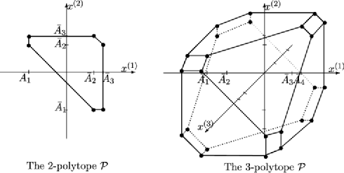
Figure 1: Examples of the admissible domain in the cases $k=3$ and $k=4$.

The result of Theorem 3 demonstrates that the boundary of $\Omega\subset\mathbf{R}^{k-1}$ consists of lower dimensional polytopes, each made up of a cross product of two sets of dimension $l-1$ and $k-l-1$, for $l=1,\ldots,k-1$. These correspond to the restriction of the permutations in each block to the smallest or largest $l-1$ elements of the block and their complements. The functions $\Lambda_{1}$ and $\Lambda_{2}$ are defined on these subsets as is $\Lambda$ in (2). To illustrate this, in Figure 1 we have given two diagrams showing the polytope $\mathcal{P}$ for the cases $k=3$ and $k=4$. In the first picture, we have 6 vertexes and 6 sides with boundaries made up of lines representing the dimension reduction to one dimension. In this case, one of $\Lambda_{1}$ and $\Lambda_{2}$ is identically zero. In the second picture, the two-dimensional boundaries are either six-sided, corresponding to one of $\Lambda_{1}$ and $\Lambda_{2}$ being identically zero, and the other a two-dimensional function, or are rectangles corresponding to both $\Lambda_{1}$ and $\Lambda_{2}$ being one-dimensional functions.

4 Saddlepoint approximations for $\Lambda$

Consider $\mathrm{P}(\Lambda(\bar{X})\geq u^{2}/2)$, where $\mathrm{P}$ denotes the conditional distribution given $A$, and define

$$r(x)=e^{-b\Lambda(x)}(2\pi/b)^{-k/2}\bigl{|}\kappa^{\prime\prime}(t_{x})\bigr{|}^{-1/2}$$

for $x\in\Omega$. In the case of identically distributed random vectors ${X}_{i}=(X_{i1},\break\ldots,X_{i,k-1})\in\Omega$, $i=1,\ldots,N$ with known densities, $r(\bar{X})$ is a saddlepoint density approximation for $\bar{X}$, obtained by Borovkov and Rogozin (1965). In our case, the lack of a density requires the application of Theorem 1 of Kolassa and Robinson (2011). We consider

$$\mathrm{P}\bigl{(}\Lambda(\bar{X})\geq u^{2}/2\bigr{)}=\mathrm{P}(\bar{X}\in\mathcal{F}),$$

where $\mathcal{F}=\{x\dvtx\Lambda(x)\geq u^{2}/2\}$ and $u\in\Omega_{-\varepsilon}=(\Omega_{\varepsilon}^{c})^{c}=\{x\in\mathbf{R}^{k-1},y\in\Omega^{c}\dvtx|x-y|<\varepsilon\}^{c}$. Whenever $\mathcal{F}^{c}\subset\Omega_{-\varepsilon}$, our case must only meet the necessary conditions (A1)–(A4) stated in Kolassa and Robinson (2011). The cumulative generating function (1) exists throughout $\mathbf{R}^{k-1}$, therefore, the first condition is met. The average variance $\kappa^{\prime\prime}(t)$ is a positive definite matrix which equals the identity matrix at the origin. Thus, the second condition is met. The third condition only requires the existence of some moments and the fourth is a smoothness condition, which we assume holds. It will hold, for example, if the observations are from a distribution with a continuous component. Thus we can apply Theorems 1 and 2 of Kolassa and Robinson (2011) as in that paper to get the following result.

Theorem 4.

For $\varepsilon>0$ and $u^{2}/2<\log k-\varepsilon$, under conditions (A1)–(A4) of Kolassa and Robinson (2011),

$$\qquad\mathbf{P}\bigl{(}\Lambda(\bar{X})\geq u^{2}/2\bigr{)} = Q_{k-1}\bigl{(}bu^{2}\bigr{)}\bigl{(}1+O(1/b)\bigr{)}+\frac{c_{b}}{b}u^{k-1}e^{-{bu^{2}}/{2}}\frac{G(u)-1}{u^{2}},$$ (5)

$$\mathbf{P}\bigl{(}\Lambda(\bar{X})\geq u^{2}/2\bigr{)} = Q_{k-1}\bigl{(}bu^{*2}\bigr{)}\bigl{(}1+O(1/b)\bigr{)},$$ (6)

where

$$Q_{k-1}(x)=\mathrm{P}\bigl{(}\mathcal{X}^{2}_{k-1}\geq x\bigr{)}=\frac{1}{2^{(k-1)/2}\Gamma((k-1)/2)}\int_{x}^{\infty}z^{(k-1)/2-1}e^{-z/2}\,dz,$$

$u^{*}=u-\log(G(u))/bu$, $c_{b}=b^{{(k-1)}/{2}}/2^{{(k-3)}/{2}}\Gamma(\frac{k-1}{2})$,

$$\delta(u,s)=\frac{\Gamma({(k-1)}/{2})|\kappa^{\prime\prime}(t_{x})|^{-{1}/{2}}|\kappa^{\prime\prime}(0)|^{{1}/{2}}r^{k-2}}{2\pi^{{(k-1)}/{2}}u^{k-3}|s^{T}\kappa^{\prime\prime}(0)^{{1}/{2}}t_{x}|}$$

and

$$G(u)=\int_{S_{k-1}}\delta(u,s)\,ds,$$

for $S_{k-1}$ the $k-1$-dimensional unit sphere centered at zero, and where, for each $s\in S_{k-1}$, $r$ is chosen so $\Lambda(r\kappa^{\prime\prime}(0)^{1/2}s)=u^{2}/2$. Here, $t_{x}$ is a solution to (3) at the point $x=r\kappa^{\prime\prime}(0)^{1/2}s$.

We note that the constraint $u^{2}/2<\log k-\varepsilon$, ensures that the level set of $\Lambda(x)$ corresponding to $u$ lies entirely in $\Omega$, since the minimum value of $\Lambda(x)$ for an $x$ on the boundary occurs for $l=1$ and $\Lambda_{1}(x)=\Lambda_{2}(x)=0$ in Theorem 3. The remainder of the proof then follows in the same way as in Theorem 2 of Kolassa and Robinson (2011), so we omit it. The theorem gives approximations of the tail probabilities of the test statistic $\Lambda$ under permutations, in forms like those of Lugananni–Rice and Barndorff–Nielsen in the one-dimensional case.

Table 1: Accuracy for exponentially squared errors, $b=10$ and $k=4$

$\bolds{u}$	0.6	0.8	1.0	1.2	1.4
MC $F$	0.3353	0.1042	0.0257	0.0047	0.0003
$F$	0.3286	0.1193	0.0342	0.0083	0.0018
MC $\Lambda$	0.4494	0.1777	0.0455	0.0071	0.0008
SP LR	0.4179	0.1645	0.0480	0.0070	0.0007
SP BN	0.4059	0.1565	0.0441	0.0066	0.0007

Table 2: Accuracy for exponential squared errors, $b=5$ and $k=3$

$\bolds{u}$	0.6	0.8	1.0	1.2	1.4
MC $F$	0.4620	0.2448	0.1277	0.0653	0.0427
$F$	0.4441	0.2603	0.1434	0.0767	0.0408
MC $\Lambda$	0.5118	0.3133	0.1578	0.0774	0.0270
SP LR	0.5011	0.2988	0.1563	0.0736	0.0278
SP BN	0.4950	0.2917	0.1500	0.0687	0.0255

5 Numerical results

5.1 Accuracy

For each of the simulation experiments, we obtained a single matrix $A$ by sampling from a distribution, that of squared exponential random variables for our Tables 1, 2 and 3. Then we used 100,000 replicates of random permutations of each block to obtain Monte Carlo approximations to the tail probabilities of the permutation tests for the statistics $F$ and $\Lambda$, shown as $\mathrm{MC}$ $F$ and $\mathrm{MC}$ $\Lambda$ in the tables. We compared these to the tail probabilities from the $F$ distribution for the $F$-statistic and to the saddlepoint approximations for the $\Lambda$ statistic obtained using formulas (5) (SP LR) and (6) (SP BN), respectively, with $100$ Monte Carlo samples used to approximate integrals on the sphere $S_{k-1}$, as in the Remark in Section 2 of Kolassa and Robinson (2011). We also used the method from Genz (2003), for approximation of the integral on the sphere, obtaining effectively the same accuracy as with Monte Carlo sampling.

From Tables 1 and 2, we note that the accuracy is high for the $\Lambda$ test, even for only 5 blocks of size 3. We note that for Table 2 the theorem holds for $u$ less than $\sqrt{2\log 3}=1.48$, so we are restricted to this region. Results from other simulations show even greater accuracy under normal errors or errors that are not from long tailed distributions.

The $F$-statistic has less accuracy in the tails, partly because the $F$-statistic approximates the average of tail probabilities conditioned on the matrix $A$, using $100\mbox{,}000$ permutations for each $A$, so that even in the case of normal errors, it may not agree with the conditional tail probabilities approximated by $\mathrm{MC}$ $F$-values from the tables of this section, which give proportions in the tails obtained from $100\mbox{,}000$ Monte Carlo simulations from a particular sample and is an approximation of the conditional distribution. To consider the accuracy of the unconditional test, we obtained 1000 replicates from each of a normal and exponential squared distribution, obtained tail probabilities for these from the permutation test for the $F$-statistic, averaged these over the 1000 replicates and compared these approximations to the $F$ distribution. In the normal case, the results were very accurate, essentially replicating the theoretical results, as expected, and for the squared exponential case the results are given in Table 3 indicating that errors remain unsatisfactory in the tails.

Table 3: Average of 1000 permutation test results for exponential squared errors with $b=10$ and $k=4$ compared to the $F$ distribution

$\bolds{u}$	0.6	0.8	1.0	1.2	1.4
$E$ MC $F$	0.3175	0.0836	0.0171	0.0032	0.0005
$F$	0.3286	0.1193	0.0342	0.0083	0.0018

5.2 Power results for the saddlepoint approximations

We compare the $F$-statistic and the saddle point approximations using (5) and (6) using $100$ Monte Carlo uniform samples from $S_{k}$. There were $2000$ samples with errors drawn from the exponential and the exponential squared distributions, and for each of these $p$-values were calculated using the saddlepoint approximations for the $\Lambda$ statistic obtained using formulas (5) (PowerLR) and (6) (PowerBN), respectively, and using $10\mbox{,}000$ permutations to approximate the $p$-values for the $F$-statistic, for a design with $10$ blocks of size $4$. We selected treatment effects $\mu$, as $(0,0,0,0),(-1/5,0,0,1/5),\ldots,(-9/5,0,0,9/5)$.

Under the exponential distribution, in Table 4, the $\Lambda$-statistic gives a slight increase in power compared to $F$-statistic for small $\sum\mu^{2}$ and under the exponentially squared distribution, in Table 5, the $\Lambda$-statistic gives a substantial increase in power compared to $F$-statistic for moderate values of $\sum\mu^{2}$. In both cases there is no difference for higher powers. We note that the tests have essentially equal power up to computational accuracy under the Normal, Uniform and Gamma (shape parameter 5) distributions. The increase in power becomes noticeable in long tail distributions like Exponential, Exponential Squared, Gamma (shape parameter 0.5) distributions.

Table 4: Power calculation under the exponential distribution

$\bm{\sum}\bolds{\mu^{2}}$	0.0	0.04	0.16	0.36	0.64	1.0	1.44	1.96
PowerF	0.056	0.081	0.209	0.424	0.668	0.861	0.982	1
PowerLR	0.049	0.091	0.235	0.451	0.679	0.862	0.981	1
PowerBN	0.053	0.093	0.238	0.455	0.681	0.866	0.982	1

Table 5: Power calculation under the exponentially squared distribution

$\bolds{\sum\mu^{2}}$	0.0	0.04	0.16	0.36	0.64	1.0	1.44	1.96
PowerF	0.051	0.101	0.230	0.490	0.711	0.840	0.987	1
PowerLR	0.057	0.169	0.319	0.545	0.727	0.832	0.976	1
PowerBN	0.063	0.178	0.328	0.550	0.731	0.832	0.977	1

6 Proofs of theorems of Section 3

Proof of Theorem 1 From (3), $\Omega=\{x\dvtx\kappa^{\prime}(t)=x,\mbox{ for some }t\in\mathbf{R}^{k-1}\}$, the image of $\kappa^{\prime}(\cdot)$. Using equation (1) we get the $j$th component of $\kappa^{\prime}(t)$,

$$\kappa^{\prime}_{j}(t)=\frac{1}{b}\sum_{i=1}^{b}\frac{\sum_{\pi\in\Pi}a_{i\pi(j)}\exp(t^{T}a_{i\pi})}{\sum_{\pi\in\Pi}\exp(t^{T}a_{i\pi})}.$$

Here, $a_{i\pi(j)}$ is the $j$th component of $a_{i\pi}$ and

$$\bar{A}_{1}=\frac{1}{b}\sum_{i=1}^{b}a_{i1}<\frac{1}{b}\sum_{i=1}^{b}\frac{\sum_{\pi\in\Pi}a_{i\pi(j)}\exp(t^{T}a_{i\pi})}{\sum_{\pi\in\Pi}\exp(t^{T}a_{i\pi})}<\frac{1}{b}\sum_{i=1}^{b}a_{ik}=\bar{A}_{k}.$$

Using the same approach, we can conclude that for all distinct integers $j_{1}$, $j_{2},\ldots,j_{k-1}$ taking values $1,2,\ldots,k-1$, and for $l=1,\ldots,k-1$,

$$\sum_{j=1}^{l}\bar{A}_{j}<\frac{1}{b}\sum_{i=1}^{b}\frac{\sum_{\pi\in\Pi}\sum_{m=1}^{l}a_{i\pi(j_{m})}\exp(t^{T}a_{i\pi})}{\sum_{\pi\in\Pi}\exp(t^{T}a_{i\pi})}<\sum_{j=k-l+1}^{k}\bar{A}_{j}.$$ (7)

So $\Omega\subset\mathcal{P}$.

Let us prove that $\Omega$ is a convex set. Let $x,y\in\Omega$ and $c+d=1$, $c$, $d>0$. Then for all $t\in\mathbf{R}^{k-1}$

$$t^{T}(cx+dy)-\kappa(t)=c\bigl{(}t^{T}x-\kappa(t)\bigr{)}+d\bigl{(}t^{T}y-\kappa(t)\bigr{)}\leq c\Lambda(x)+d\Lambda(y)<\infty.$$

Since the expression $t^{T}(cx+dy)-\kappa(t)$ is bounded and convex, it has a maximum, so that $cx+dy\in\Omega$ and

$$\Lambda(cx+dy)\leq c\Lambda(x)+d\Lambda(y),$$

so $\Omega$ is convex.

To see that each vertex of the polytope is a limiting point of $\Omega$, consider any vertex $\bar{A}_{\hat{\pi}}=(\bar{A}_{\hat{\pi}(1)},\bar{A}_{\hat{\pi}(2)},\ldots,\bar{A}_{\hat{\pi}(k-1)})$. Suppose $\hat{\pi}(k)=j$ and define $l_{1},\ldots,l_{k}$ such that $\hat{\pi}(l_{i})=i$, so $l_{j}=k$. We can show that

$$\lim_{t_{l_{j+1}}\to\infty}\cdots\lim_{t_{l_{k}}\to\infty}\lim_{t_{l_{j-1}}\to-\infty}\cdots\lim_{t_{l_{1}}\to-\infty}\kappa^{\prime}(t)=(\bar{A}_{\hat{\pi}(1)},\ldots,\bar{A}_{\hat{\pi}(k-1)}).$$ (8)

To see this, write

$$\kappa^{\prime}(t) = \frac{1}{b}\sum_{i=1}^{b}\frac{\sum_{\pi\in\Pi}a_{i\pi}\exp(t^{T}(a_{i\pi}-a_{i\hat{\pi}}))}{\sum_{\pi\in\Pi}\exp(t^{T}(a_{i\pi}-a_{i\hat{\pi}}))}$$

$$= \frac{1}{b}\sum_{i=1}^{b}\frac{a_{i\hat{\pi}}+\sum_{\pi\in\Pi,\pi\neq\hat{\pi}}a_{i\pi}\exp(t^{T}(a_{i\pi}-a_{i\hat{\pi}}))}{1+\sum_{\pi\in\Pi,\pi\neq\hat{\pi}}\exp(t^{T}(a_{i\pi}-a_{i\hat{\pi}}))}.$$

Note that $a_{i\hat{\pi}(l_{1})}=a_{i1}$ is the smallest entry in the $i$th row so the coefficient of $t_{l_{1}}$, $a_{i\pi(l_{1})}-a_{i\hat{\pi}(l_{1})}=a_{i\pi(l_{1})}-a_{i1}$, is either positive or zero for any $\pi\in\Pi$. As $t_{l_{1}}\to-\infty$, only the permutations with $\pi(l_{1})=1$ give nonzero terms, so

$$\qquad\lim_{t_{l_{1}}\to-\infty}\kappa^{\prime}(t)=\frac{1}{b}\sum_{i=1}^{b}\frac{a_{i\hat{\pi}}+\sum_{\pi\in\{\Pi\dvtx\pi(l_{1})=1\},\pi\neq\hat{\pi}}a_{i\pi}\exp(t^{T}(a_{i\pi}-a_{i\hat{\pi}}))}{1+\sum_{\pi\in\{\Pi\dvtx\pi(l_{1})=1\},\pi\neq\hat{\pi}}\exp(t^{T}(a_{i\pi}-a_{i\hat{\pi}}))}.$$ (10)

Continuing to take limits, in the order given in (8), removes all but the first term in the numerator and denominator of (10), to prove (8). Thus, the vertex $\bar{A}_{\hat{\pi}}$ is a limiting point of $\Omega$. Since $\hat{\pi}$ is arbitrary, this holds for each vertex of the polytope. Since $\Omega$ is a convex set enclosed by the edges of the polytope, $\Omega$ is the interior of the polytope.

Proof of Theorem 2 Consider the expression $t^{T}x-\kappa(t)$. Using previous notation set $x=\bar{A}_{\hat{\pi}}$. Using the definition (1), we can write

$$t^{T}\bar{A}_{\hat{\pi}}-\kappa(t)=-\frac{1}{b}\sum_{i=1}^{b}\log\frac{1}{k!}\sum_{\pi\in\Pi}e^{t^{T}(a_{i\pi}-a_{i\hat{\pi}})},$$ (11)

since $\bar{A}_{\hat{\pi}}=\frac{1}{b}\sum_{i=1}^{b}a_{i\hat{\pi}}$. Then by the same argument used in Theorem 1, we get

$$\lim_{t_{l_{j+1}}\to\infty}\cdots\lim_{t_{l_{k}}\to\infty}\lim_{t_{l_{j-1}}\to-\infty}\cdots\lim_{t_{l_{1}}\to-\infty}\bigl{[}t^{T}\bar{A}_{\hat{\pi}}-\kappa(t)\bigr{]}=\log k!.$$

From the definition of supremum and equation (2),

$$\Lambda(x)=\sup_{t}\bigl{\{}t^{T}\bar{A}_{\hat{\pi}}-\kappa(t)\bigr{\}}=\log k!.$$

Since $\hat{\pi}$ is chosen arbitrarily $\Lambda(x)$ is equal to $\log k!$ on all vertexes. These are the extreme points of $\Omega$ and $\Lambda(x)$ is convex, so $\Lambda(x)$ takes its maximum on the vertexes and is finite on all points of $\mathcal{P}$ and so on the boundary of $\Omega$.

Proof of Theorem 3 Using (4), choose $x$ so that

$$\sum_{j=1}^{l}x_{s_{j}}=\sum_{j=1}^{l}\bar{A}_{j}$$

is true for some $\{s_{j}\}$ and $l$. The alternative choice will follow in the same way. So

$$x^{T}t=\sum_{j=1}^{l-1}x_{s_{j}}(t_{s_{j}}-t_{s_{l}})+\sum_{j=1}^{l}\bar{A}_{j}t_{s_{l}}+\sum_{j=l+1}^{k-1}x_{s_{j}}t_{s_{j}}$$

and, from (1), $\kappa(t)$ can be written

$$\frac{1}{b}\sum_{i=1}^{b}\log\frac{1}{k!}\sum_{\pi\in\Pi}\exp\Biggl{(}{\sum_{j=1}^{l-1}a_{i\pi(j)}(t_{s_{j}}-t_{s_{l}})+\sum_{j=1}^{l}a_{i\pi(j)}t_{s_{l}}+\sum_{j=l+1}^{k-1}a_{i\pi(j)}t_{s_{j}}}\Biggr{)}.$$

Make the substitution

$$u_{j}=\cases{t_{s_{j}}-t_{s_{l}},&\quad$\mbox{for }1\leq j<l,$\vspace*{2pt}\cr t_{s_{j}},&\quad$\mbox{for }l\leq j\leq k-1,$}$$

and use the first equality in (4), to write $x^{T}t-\kappa(t)$ as

$$\sum_{j=1,j\neq l}^{k-1}x_{s_{j}}u_{j}-\frac{1}{b}\sum_{i=1}^{b}\log\frac{1}{k!}\sum_{\pi\in\Pi}\exp\Biggl{(}\sum_{j=1,j\neq l}^{k-1}a_{i\pi(j)}u_{j}+u_{l}\sum_{j=1}^{l}(a_{i\pi(j)}-a_{ij})\Biggr{)},$$

where for each $1\leq j\leq l$, $\sum_{j=1}^{l}(a_{i\pi(j)}-a_{ij})\geq 0$. Let $u_{l}\to-\infty$ and we have

$$\lim_{u_{l}\to-\infty}\bigl{(}x^{T}t-\kappa(t)\bigr{)}=\sum_{j=1,j\neq l}^{k-1}x_{s_{j}}u_{j}-\frac{1}{b}\sum_{i=1}^{b}\log\frac{1}{k!}\sum_{\pi\in\hat{\Pi}}\exp\Biggl{(}\sum_{j=1,j\neq l}^{k-1}a_{i\pi(j)}u_{j}\Biggr{)},$$

where $\hat{\Pi}=\{\pi\in\Pi\dvtx\sum_{j=1}^{l}(a_{i\pi(j)}-a_{ij})=0\}$. Let $\hat{\Pi}_{1}$ and $\hat{\Pi}_{2}$ be sets of all permutations $\hat{\pi}_{1}$ and $\hat{\pi}_{2}$ of integers $\{1,\ldots,l\}$ and $\{l+1,\ldots,k\}$, respectively. Then the above expression can be rewritten

$$\lim_{u_{l}\to-\infty}\bigl{(}x^{T}t-\kappa(t)\bigr{)} = \sum_{j=1}^{l-1}x_{s_{j}}u_{j}-\frac{1}{b}\sum_{i=1}^{b}\log\frac{1}{l!}\sum_{\hat{\pi}_{1}\in\hat{\Pi}_{1}}e^{\sum_{j=1}^{l-1}a_{i\hat{\pi}_{1}(j)}u_{j}}$$

$${}+\sum_{j=l+1}^{k-1}x_{s_{j}}u_{j}-\frac{1}{b}\sum_{i=1}^{b}\log\frac{1}{(k-l)!}\sum_{\hat{\pi}_{2}\in\hat{\Pi}_{2}}e^{\sum_{j=l+1}^{k-1}a_{i\hat{\pi}_{2}(j)}u_{j}}$$

$${}+\log\frac{k!}{l!(k-l)!}.$$

Now taking suprema over $u_{1},\ldots,u_{l-1}$ and $u_{l+1},\ldots,u_{k-1}$ in the first two terms on the right in (6), the statement of the theorem follows.

References

- Borovkov and Rogozin (1965) {barticle}[author] \bauthor\bsnmBorovkov, \bfnmA. A.\binitsA. A. and \bauthor\bsnmRogozin, \bfnmB. A.\binitsB. A. (\byear1965). \btitleOn the multi-dimensional central limit theorem. \bjournalTheory Probab. Appl. \bvolume10 \bpages55–62. \bptokimsref\endbibitem
- Brown and Maritz (1982) {barticle}[mr] \bauthor\bsnmBrown, \bfnmB. M.\binitsB. M. and \bauthor\bsnmMaritz, \bfnmJ. S.\binitsJ. S. (\byear1982). \btitleDistribution-free methods in regression. \bjournalAustral. J. Statist. \bvolume24 \bpages318–331. \bidissn=0004-9581, mr=0694150 \bptokimsref\endbibitem
- Fisher (1935) {bbook}[author] \bauthor\bsnmFisher, \bfnmRonald A.\binitsR. A. (\byear1935). \btitleThe Design of Experiments. \bpublisherOliver and Boyd, \baddressEdinburgh. \bptokimsref\endbibitem
- Genz (2003) {barticle}[mr] \bauthor\bsnmGenz, \bfnmAlan\binitsA. (\byear2003). \btitleFully symmetric interpolatory rules for multiple integrals over hyper-spherical surfaces. \bjournalJ. Comput. Appl. Math. \bvolume157 \bpages187–195. \biddoi=10.1016/S0377-0427(03)00413-8, issn=0377-0427, mr=1996475 \bptokimsref\endbibitem
- Jin and Robinson (1999) {barticle}[mr] \bauthor\bsnmJin, \bfnmRungao\binitsR. and \bauthor\bsnmRobinson, \bfnmJohn\binitsJ. (\byear1999). \btitleSaddlepoint approximation near the endpoints of the support. \bjournalStatist. Probab. Lett. \bvolume45 \bpages295–303. \biddoi=10.1016/S0167-7152(99)00071-1, issn=0167-7152, mr=1734610 \bptokimsref\endbibitem
- Kolassa and Robinson (2011) {barticle}[mr] \bauthor\bsnmKolassa, \bfnmJohn\binitsJ. and \bauthor\bsnmRobinson, \bfnmJohn\binitsJ. (\byear2011). \btitleSaddlepoint approximations for likelihood ratio like statistics with applications to permutation tests. \bjournalAnn. Statist. \bvolume39 \bpages3357–3368. \biddoi=10.1214/11-AOS945, issn=0090-5364, mr=3012411 \bptokimsref\endbibitem
- Robinson (1982) {barticle}[mr] \bauthor\bsnmRobinson, \bfnmJ.\binitsJ. (\byear1982). \btitleSaddlepoint approximations for permutation tests and confidence intervals. \bjournalJ. R. Stat. Soc. Ser. B Stat. Methodol. \bvolume44 \bpages91–101. \bidissn=0035-9246, mr=0655378 \bptokimsref\endbibitem