Mean-field electrostatics beyond the point-charge description

Abstract

This review explores the number of mean-field constructions for ions whose structure goes beyond the point-charge description, a representation used in the standard Poisson-Boltzmann equation. The exploration is motivated by a body of experimental work which indicates that ion-specific effects play a significant role, where ions of the same valence charge but different size, polarizability, or shape yield quite different, and sometimes surprising results. Furthermore, there are many large ions encountered in soft-matter and biophysics that do not fit into a point-charge description, and their extension in space and shape must be taken into account of any reasonable representation.

I Introduction

The present review explores the number of mean-field constructions for ions whose structure goes beyond the point-charge description, the representation used in the standard Poisson-Boltzman equation. The structural details neglected by a point-charge picture can be related to electrostatic structure of an ion, and they lead to polarizability, asymmetric interactions, or softening of Coulomb interactions if a distribution of an ion charge is extended in space, or they can be linked to the Pauli exclusion principle, and lead to the excluded volume effects or other softer types of repulsive interactions.

The interest in incorporating these details came with the observation that charge is not the sole parameter that describes an ion David09 , as various ion-specific effects emerged in experimental work, beginning with the now famous work of Hofmeister Hofmeister . In the Hofmeister series ions of the same valance number can be arranged into a sequence according to what effect they have on protein solubility. The larger and more polarizable ions weaken hydrophobicity of a protein, while the smaller ones strengthen it Zhang06 . Fluid interfaces is another place where ion specificity plays an important role in regulating a surface tension Yan10 . Dielectric decrement of an electrolyte upon addition of a salt is yet another example where specificity of an ion can be measured Collie48 ; David11 and that is associated with how a given ion affects a water structure.

Another motivation for a model with structured particles is to come up with a more realistic description for water, which within the standard Poisson-Boltzmann equation is represented as a background dielectric constants David07 . A polar solvent dissociates salts and dissolves ions, but electrostatic interactions between dissolved ions are not the same as in vacuum. The solvent background screens interactions as dipoles of a solvent molecules align themselves along field lines coming from ion centers. This type of screening can be represented as an increased dielectric constant of a background, which is about eighty times larger than that in vacuum. This description is accurate if alignment of solvent molecules is proportional to electrostatic field. But the proportionality relation breaks down when alignment becomes complete and solvent no longer responds to an external field, thus the screening effect slowly goes away.

Finally, as a number of problems in soft-matter and biophysics increases and involves larger ions with significant size and definite shape, a point-charge representation no longer serves as an accurate representation. Charge of an ion has to be represented as extended in space in order to capture novel results that such ions give rise to Pincus08 .

The mean-field approximation is a powerful method and yet very simple. It represents pair interactions as an effective one-body external potential,

$$w({\bf r})=\int d{\bf r}^{\prime}\rho({\bf r}^{\prime})u({\bf r},{\bf r}^{\prime}),$$ (1)

which is a mean-potential a particle feels due to other particles in a system. $u({\bf r},{\bf r}^{\prime})$ is the true pair interaction and $\rho({\bf r})$ is the equilibrium density of all particles. To construct a number density we write

$$\rho({\bf r})=\rho_{b}e^{\beta w_{b}}e^{-\beta[V({\bf r})+w({\bf r})]},$$ (2)

where $\rho_{b}$ and $w_{b}$ is the value of $\rho({\bf r})$ and $w({\bf r})$ in a bulk, and $V({\bf r})$ is the external potential. The density now needs to be obtained self-consistently.

The mean-field approximation includes particle interactions, and this is what sets it apart from the ideal-gas model, but it neglects correlations since it assumes that each particle interacts with a frozen distribution of particles that does not change with the location of a test particle at ${\bf r}$. The test particle in this sense is invisible: it measures but does not disturb the system. How accurate the mean-field is will depend on how negligible correlations are Netz00a . Among theoretical systems for which the mean-field yields exact density profile are the hard-sphere system in the infinite dimension limit Klein86 , and the system of particles interacting via potential of the form $U({r})=\lambda^{3}u(\lambda r)$ in the limit $\lambda\to 0$, where $u(r)$ is bounded and with finite range Klein77b . For physically relevant systems $\lambda$ remains finite, and so the corrections to the mean-field are always present and real. An example of a system that is regarded as weakly-correlated liquid is the Gaussian core model at room temperature and so it is very accurately represented by the mean-field approximation Hansen00b .

Correcting the mean-field with consecutive perturbative terms makes sense up to some value of an expansion parameter. At some point this no longer makes sense and electrostatics enters into the strong-coupling limit. This splits electrostatics into two ”worlds” Rudi10 . In the strong-coupling ”wonder world” things stand up on their head: the same-charged particles attract each other Linse99 , for a counterion only system the distribution of counterions near a charged wall falls off exponentially as in the ideal-gas model Shklovskii99a ; Shklovskii99b ; Netz00b ; Trizac11 . The mean-field approximation has nothing to say in this regime Bloomfield96 ; Yan02 ; Shklovskii02 .

II The mean-field approximation

In this section we go over the mean-field approximation by starting from a complete partition function. To proceed, we postulate the system with scaled particle interactions, $u_{\lambda}({\bf r},{\bf r}^{\prime})=\lambda u({\bf r},{\bf r}^{\prime})$, where $\lambda=0$ corresponds to the ideal-gas limit, and $\lambda=1$ recovers the true system. The partition function for this system reads

$$Z_{\lambda}=\frac{1}{N!\Lambda^{3N}}\int\prod_{i=1}^{N}d{\bf r}_{i}e^{-\beta\sum_{i<j}\lambda u({\bf r}_{i},{\bf r}_{j})}e^{-\beta\sum_{i}V_{\lambda}({\bf r}_{i})},$$ (3)

where $V_{\lambda}$ is the $\lambda$-dependent external potential. Its precise form is not required as it will not appear in the final expression. It suffices to know that the sole function of $V_{\lambda}$ is to maintain the equilibrium density $\lambda$-independent, $\rho_{\lambda}=\rho$, so that the density always corresponds to a physical system. $\Lambda$ in the partition function is a length scale, and $\beta=1/(k_{B}T)$.

The free energy is obtained from thermodynamic integration,

$$F = F_{\lambda=0}+\int_{0}^{1}d\lambda\,\frac{\partial F_{\lambda}}{\partial\lambda},$$ (4)

where $\beta F_{\lambda}=-\log Z_{\lambda}$, $F_{\lambda=0}=F_{\rm id}+\int d{\bf r}\,\rho({\bf r})V_{\lambda=0}({\bf r})$, and the ideal-gas contribution to the free energy is

$$\beta F_{\rm id}=\int d{\bf r}\,\rho\Big{(}\log\rho\Lambda^{3}-1\Big{)}.$$ (5)

The integrand in the free energy expression is

$$\frac{\partial F_{\lambda}}{\partial\lambda} = \int d{\bf r}\,\rho({\bf r})\frac{\partial V_{\lambda}({\bf r})}{\partial\lambda}$$ (6)

$$+ \frac{1}{2}\int d{\bf r}\int d{\bf r}^{\prime}\,\rho({\bf r})\rho({\bf r}^{\prime})u({\bf r},{\bf r}^{\prime})$$

$$+ \frac{1}{2}\int d{\bf r}\int d{\bf r}^{\prime}\,\rho({\bf r})\rho({\bf r}^{\prime})u({\bf r},{\bf r}^{\prime})h_{\lambda}({\bf r},{\bf r}^{\prime}),$$

where $h_{\lambda}$ is the $\lambda$-dependent correlation function. After insertion into the free energy expression we find

$$F = F_{\rm id}+\int d{\bf r}\,\rho({\bf r})V({\bf r})+\frac{1}{2}\int d{\bf r}\int d{\bf r}^{\prime}\,\rho({\bf r})\rho({\bf r}^{\prime})u({\bf r},{\bf r}^{\prime})$$

$$+ \frac{1}{2}\int d{\bf r}\int d{\bf r}^{\prime}\,\rho({\bf r})\rho({\bf r}^{\prime})u({\bf r},{\bf r}^{\prime})\int_{0}^{1}d\lambda\,h_{\lambda}({\bf r},{\bf r}^{\prime}),$$

where the $\lambda$-dependent external potential disappears from the final expression.

The mean-field approximation is obtained by setting correlations to zero, $h_{\lambda}=0$,

$$F_{\rm mf} = F_{\rm id}+\int d{\bf r}\,V({\bf r})\rho({\bf r})+\frac{1}{2}\int d{\bf r}\int d{\bf r}^{\prime}\,\rho({\bf r})\rho({\bf r}^{\prime})u({\bf r},{\bf r}^{\prime}),$$ (8)

where the neglected correlation term is

$$F_{c}=\frac{1}{2}\int d{\bf r}\int d{\bf r}^{\prime}\,\rho({\bf r})\rho({\bf r}^{\prime})u({\bf r},{\bf r}^{\prime})\int_{0}^{1}d\lambda\,h_{\lambda}({\bf r},{\bf r}^{\prime}).$$ (9)

How accurate the mean-field is depends on the value of $F_{c}$.

The mean-field free energy is written as a functional of a density that is not known a priori. It has to be obtained variationally, knowing that it minimizes the free energy, a condition expressed as functional derivative,

$$\frac{\delta F}{\delta\rho({\bf r})}=0,$$ (10)

which yields

$$\rho({\bf r})=\rho_{b}e^{\beta w_{b}}e^{-\beta V({\bf r})-\beta\int d{\bf r}^{\prime}\,\rho({\bf r}^{\prime})u({\bf r},{\bf r}^{\prime})},$$ (11)

where $w_{b}=\rho_{b}\int d{\bf r}^{\prime}\,u({\bf r},{\bf r}^{\prime})$ and ensures that a correct bulk limit is recovered.

Something more needs to be said about correlations. We have seen how correlations are eliminated from free energy. Explicitly, thus, correlations are not part of the description. However, implicitly they are there. If we take the exact relation,

$$-\frac{\delta\rho({\bf r})}{\delta\beta V({\bf r}^{\prime})}=\rho({\bf r}^{\prime})\rho({\bf r}^{\prime})h({\bf r},{\bf r}^{\prime})+\rho({\bf r})\delta({\bf r}-{\bf r}^{\prime}),$$ (12)

which can be verified from complete partition function, we should expect that the mean-field density in Eq. (11) would yield

$$-\frac{\delta\rho({\bf r})}{\delta\beta V({\bf r}^{\prime})}=\rho({\bf r})\delta({\bf r}-{\bf r}^{\prime}),$$ (13)

since correlations were set to zero. Indeed, this is what one gets for an ideal-gas. But the mean-field density leads instead to a self-consistent equation indicating the presence of correlations,

$$-\frac{\delta\rho({\bf r})}{\delta\beta V({\bf r}^{\prime})}=\rho({\bf r})\delta({\bf r}-{\bf r}^{\prime})+\int d{\bf r}^{\prime\prime}\,\beta u({\bf r},{\bf r}^{\prime\prime})\frac{\delta\rho({\bf r}^{\prime\prime})}{\delta\beta V({\bf r}^{\prime})}.$$ (14)

In combination with Eq. (12) it can be put into the Ornstein-Zernike equation format,

$$h({\bf r},{\bf r}^{\prime})=-\beta u({\bf r},{\bf r}^{\prime})-\int d{\bf r}^{\prime\prime}\,\rho({\bf r}^{\prime\prime})h({\bf r}^{\prime},{\bf r}^{\prime\prime})\beta u({\bf r},{\bf r}^{\prime\prime}),$$ (15)

where the direct correlation function in the mean-field is approximated as

$$c({\bf r},{\bf r}^{\prime})=-\beta u({\bf r},{\bf r}^{\prime}).$$ (16)

III Point-ion with a structure

III.1 The standard Poisson-Boltzmann equation

Within the standard Poisson-Boltzmann equation ions are represented as point-charges. The model is constructed from the Poisson equation

$$\epsilon\nabla^{2}\psi({\bf r})=-\rho_{c}({\bf r}),$$ (17)

which expresses the relation between the electrostatic potential $\psi$ and the charge density

$$\rho_{c}({\bf r})=\sum_{i=1}^{K}q_{i}\rho_{i}({\bf r}),$$ (18)

where the subscript $i$ indicates an ion species, $K$ is the number of species, and $q_{i}$ is the charge of an ion species $i$. In the Poisson equation $\epsilon$ is a background dielectric constant representing a solvent medium. The relation makes more sense if we transform it into somewhat different format,

$$\psi({\bf r})=\int d{\bf r}^{\prime}\,\rho_{c}({\bf r}^{\prime})C({\bf r},{\bf r}^{\prime}),$$ (19)

where the Green’s function $C({\bf r},{\bf r}^{\prime})$ denotes the functional form of Coulomb interactions,

$$C({\bf r}-{\bf r}^{\prime})=\frac{1}{4\pi\epsilon|{\bf r}-{\bf r}^{\prime}|},$$ (20)

and satisfies the fundamental equation

$$\epsilon\nabla^{2}C({\bf r}-{\bf r}^{\prime})=-\delta({\bf r}-{\bf r}^{\prime}).$$ (21)

The Poisson equation seen through the format in Eq. (19) is nothing more than a restated definition of an electrostatic potential, due to some distribution in space of Coulomb charges.

Within this description different ionic species are distinguished by their valence number alone. Another approximation lies in the treatment of a solvent as a background dielectric constant $\epsilon$. This description assumes that a polarization density of a polar solvent responds linearly to an electrostatic field, ${\bf P}=\gamma{\bf E}$, where ${\bf E}=-\mbox{\boldmath$\nabla$}\psi$ is the local electrostatic field. The total dielectric constant then is $\epsilon=\epsilon_{0}+\gamma$, where $\epsilon_{0}$ is the dielectric constant in vacuum, and the action of a solvent is to screen electrostatic interactions by rising dielectric constant.

To construct the Poisson-Boltzmann equation we need an expression for the charge density in terms of an electrostatic potential. This can be obtained from the number densities, $\rho_{i}$, obtained, in turn, from the mean-potential that an ion of a species $i$ feels due to other ions in a system,

$$w_{i}({\bf r})=q_{i}\int d{\bf r}^{\prime}\,\rho_{c}({\bf r}^{\prime})C({\bf r},{\bf r}^{\prime})=q_{i}\psi({\bf r}),$$ (22)

which leads to the mean-field density,

$$\rho_{i}({\bf r})=c_{i}e^{-\beta q_{i}\psi({\bf r})},$$ (23)

where $c_{i}$ is the bulk concentration. Inserting this into the Poisson equation in Eq. (17) we arrive at the Poisson-Boltzman equation,

$$\epsilon\nabla^{2}\psi=-\sum_{i=1}^{K}c_{i}q_{i}e^{-\beta q_{i}\psi}.$$ (24)

Later in the work, we refer to the Poisson-Boltzmann equation as the PB equation.

For testing different mean-field models in this work we use the wall system where electrolyte is confined by a charged wall with a surface charge $\sigma_{c}$ to a half-space $x>0$. The PB equation reduces to 1D,

$$\epsilon\psi^{\prime\prime}=-\sum_{i=1}^{K}c_{i}q_{i}e^{-\beta q_{i}\psi}.$$ (25)

The neutrality condition,

$$\int_{0}^{\infty}dx\,\rho_{c}=-\sigma_{c},$$ (26)

fixes the boundary conditions at the location of a surface charge,

$$-\epsilon\psi^{\prime}_{w}=\sigma_{c},$$ (27)

where the subscript $w$ indicates the value of a function at a contact with a wall.

Finally, we derive the contact value theorem for the PB equation, which relates the value of a density at a wall contact to bulk properties. To proceed we multiply the Poisson-Boltzmann equation by $\psi^{\prime}$,

$$\epsilon\psi^{\prime}\psi^{\prime\prime}=-\psi^{\prime}\sum_{i=1}^{K}c_{i}q_{i}e^{-\beta q_{i}\psi},$$ (28)

and rewrite it as

$$\frac{\partial}{\partial x}\bigg{(}\frac{\epsilon}{2}\psi^{\prime 2}\bigg{)}=\frac{\partial}{\partial x}\bigg{(}k_{B}T\sum_{i=1}^{K}c_{i}e^{-\beta q_{i}\psi}\bigg{)}.$$ (29)

The right-hand side term in parentheses is $k_{B}T\rho$ where $\rho=\sum_{i=1}^{K}\rho_{i}$ is the total number density. Integrating Eq. (29) from zero to infinity and using the boundary conditions, we find

$$\rho_{w}=\rho_{b}+\frac{\beta\sigma_{c}^{2}}{2\epsilon},$$ (30)

where $\rho_{b}=\sum_{i=1}^{K}c_{i}$. In the exact contact value theorem $\rho_{b}\to P$, where $P$ is a bulk pressure. The present result reflects the ideal-gas entropy of the Poisson-Boltzmann model where $P=P_{\rm id}$.

III.2 Dipolar Poisson-Boltzmann equation

Another possible point-particle is a point-dipole. The charge distribution of a dipole is comprised of two opposite charges brought infinitesimally close to each other,

$$\lim_{\begin{subarray}{c}q\to\infty\\ \varepsilon\to 0\end{subarray}}\Big{[}q\delta({\bf r}-{\bf r}^{\prime})-q\delta({\bf r}-{\bf r}^{\prime}+\varepsilon{\bf n})\Big{]}=-(\varepsilon q)\big{[}{\bf n}\cdot\mbox{\boldmath$\nabla$}\delta({\bf r}-{\bf r}^{\prime})\big{]},$$ (31)

where ${\bf n}$ is the unit vector, and $q\varepsilon=p$ is the strength of a dipole moment. The limit $q\to\infty$ is necessary to prevent the two charges from annihilation. Because of the limits, the distribution of a dipole can be represented as a gradient of a delta function.

For the system of dipoles an additional stochastic degree of freedom comes out due to dipole orientation. A complete one particle distribution is, therefore, a function of a position and orientation, $\varrho({\bf r},{\bf n})$, which reduces to the number density

$$\rho_{i}({\bf r})=\int d{\bf p}_{i}\,\varrho_{i}({\bf r},{\bf n}).$$ (32)

A full distribution, however, is required to obtain a polarization density,

$${\bf P}({\bf r})=\sum_{i=1}^{K}p_{i}\int d{\bf n}\,\,{\bf n}\,\varrho_{i}({\bf r},{\bf n}).$$ (33)

To derive the Poisson equation for point-dipoles what is still needed is the formal expression of a charge density. Recalling that a dipole consists of two opposite charges ”glued” together, the charge density can be written as

$$\rho_{c}({\bf r}) = \sum_{i=1}^{K}p_{i}\int d{\bf n}\,\lim_{\varepsilon\to 0}\Bigg{[}\frac{\varrho_{i}({\bf r},{\bf n})-\varrho_{i}({\bf r}+\varepsilon{\bf n},{\bf n})}{\varepsilon}\Bigg{]}$$ (34)

$$= -\sum_{i=1}^{K}p_{i}\int d{\bf n}\,\Big{[}{\bf n}\cdot\mbox{\boldmath$\nabla$}\varrho_{i}({\bf r},{\bf n})\Big{]}$$

$$= -\mbox{\boldmath$\nabla$}\cdot\Bigg{[}\sum_{i=1}^{K}p_{i}\int d{\bf n}\,\,{\bf n}\,\varrho_{i}({\bf r},{\bf n})\Bigg{]}$$

$$= -\mbox{\boldmath$\nabla$}\cdot{\bf P}({\bf r}).$$

The local charge density expressed as divergence of the polarization density can be understood as a charge transfer from one volume element to another, and the non-zero $(\mbox{\boldmath$\nabla$}\cdot{\bf P})$ implies that the charge that enters a given volume element is unbalanced by the charge that leaves it. The Poisson equation for the distribution of dipoles becomes

$$\epsilon\nabla^{2}\psi=\mbox{\boldmath$\nabla$}\cdot{\bf P}.$$ (35)

To obtain the mean-field description of the present system, it is required to have an appropriate expression for ${\bf P}$. As before, we start with the expression for a mean-potential. Knowing that an energy of a dipole in an external field is $(-{\bf p}\cdot{\bf E})$, we write

$$w_{i}({\bf r},\theta)={\bf p}_{i}\cdot\mbox{\boldmath$\nabla$}\psi=-p_{i}|\mbox{\boldmath$\nabla$}\psi|\cos\theta,$$ (36)

where $\theta$ is the angle between a local field ${\bf E}$ and a dipole ${\bf p}_{i}$. The corresponding mean-field distribution is

$$\varrho_{i}({\bf r},\theta)\sim c_{i}e^{\beta p_{i}|\mbox{\boldmath$\nabla$}\psi|\cos\theta},$$ (37)

and it reduces to the mean-field number density

$$\rho_{i}({\bf r}) \sim c_{i}\int_{0}^{\pi}d\theta\,\sin\!\theta\,e^{\beta p_{i}|\mbox{\boldmath$\nabla$}\psi|\cos\!\theta}.$$ (38)

The properly normalized number density is

$$\rho_{i}({\bf r})=\frac{c_{i}\sinh\beta p_{i}|\mbox{\boldmath$\nabla$}\psi|}{\beta p_{i}|\mbox{\boldmath$\nabla$}\psi|},$$ (39)

which reduces to a bulk density $c_{i}$ as a field vanishes. If dipoles were always aligned with a local field, the number density would simply be $\rho_{i}\to c_{i}e^{\beta p_{i}|\mbox{\boldmath$\nabla$}\psi|}$. The different functional form in Eq. (39) reflects the fact that dipoles fluctuate around their preferred orientation.

It remains now to obtain an expression for the polarization density,

$${\bf P} \sim \sum_{i=1}^{K}p_{i}c_{i}\int d{\bf n}\,{\bf n}\,e^{-\beta p_{i}({\bf n}\cdot\mbox{\boldmath$\nabla$}\psi)}.$$ (40)

As the polarization vector is aligned with the field,

$${\bf P}=P\Bigg{(}\frac{\bf E}{E}\Bigg{)},$$ (41)

we write $P$ as

$$P = \sum_{i=1}^{K}c_{i}p_{i}\int_{0}^{\pi}d\theta\,\sin\theta\cos\theta e^{\beta p_{i}|\mbox{\boldmath$\nabla$}\psi|\cos\theta}$$ (42)

$$= \sum_{i=1}^{K}p_{i}\Bigg{(}\frac{c_{i}\sinh\beta p_{i}|\mbox{\boldmath$\nabla$}\psi|}{\beta p_{i}|\mbox{\boldmath$\nabla$}\psi|}\Bigg{)}\Bigg{[}\coth\beta p_{i}|\mbox{\boldmath$\nabla$}\psi|-\frac{1}{\beta p_{i}|\mbox{\boldmath$\nabla$}\psi|}\Bigg{]},$$

or,

$${\bf P}=-\bigg{(}\frac{\mbox{\boldmath$\nabla$}\psi}{|\mbox{\boldmath$\nabla$}\psi|}\bigg{)}\sum_{i=1}^{K}p_{i}\Bigg{(}\frac{c_{i}\sinh\beta p_{i}|\mbox{\boldmath$\nabla$}\psi|}{\beta p_{i}|\mbox{\boldmath$\nabla$}\psi|}\Bigg{)}{\mathcal{L}}(\beta p_{i}|\mbox{\boldmath$\nabla$}\psi|),$$ (43)

where

$${\mathcal{L}}(x)=\coth x-\frac{1}{x}$$ (44)

is the Langevin function which describes the degree of alignment of a dipole in a uniform electrostatic field. An average dipole moment of a particle of a species $i$ is given as

$$\langle p\rangle=p_{i}{\mathcal{L}(\beta p_{i}|\mbox{\boldmath$\nabla$}\psi|)}.$$ (45)

In the limit $\beta p_{i}|\mbox{\boldmath$\nabla$}\psi|\to 0$, ${\mathcal{L}}\approx\beta p_{i}|\mbox{\boldmath$\nabla$}\psi|/3$. This is reasonable as an average dipole moment should be proportional to an electrostatic field. But an alignment eventually must reach saturation and ${\mathcal{L}}$ cannot exceed $1$, where ${\mathcal{L}}=1$ signals perfect alignment. Note, however, that the limit ${\mathcal{L}}\to 1$ is approached slowly, in algebraic manner like ${\mathcal{L}}\approx 1-1/(\beta p_{i}|\mbox{\boldmath$\nabla$}\psi|)$.

We have now everything that is needed for writing down a modified PB equation for a system of dipoles,

$$\epsilon\nabla^{2}\psi=-\mbox{\boldmath$\nabla$}\cdot\Bigg{[}\mbox{\boldmath$\nabla$}\psi\sum_{i=1}^{K}p_{i}c_{i}\frac{\sinh(\beta p_{i}|\mbox{\boldmath$\nabla$}\psi|)}{\beta p_{i}|\mbox{\boldmath$\nabla$}\psi|^{2}}{\mathcal{L}}(\beta p_{i}|\mbox{\boldmath$\nabla$}\psi|)\Bigg{]}.$$ (46)

The dipolar PB equation was derived in David07 , using the field-theory formalism, and was further explored in David13 . The motivation was to treat water solvent more explicitly than as a background dielectric constant, the way it is done in the standard PB model. The standard PB equation assumes a linear and local relation between the polarization density and the electrostatic field, ${\bf P}=\gamma{\bf E}$, so that the contributions of a polar solvent are subsumed into a dielectric constant $\epsilon\to\epsilon_{0}+\gamma$. The dipolar PB equation allows us to treat a polar solvent explicitly,

$$\mbox{\boldmath$\nabla$}\cdot\Bigg{[}\Bigg{(}\epsilon_{0}+\frac{p_{0}c_{d}\,\sinh(\beta p_{0}|\mbox{\boldmath$\nabla$}\psi|)}{\beta p_{0}|\mbox{\boldmath$\nabla$}\psi|^{2}}{\mathcal{L}}(\beta p_{0}|\mbox{\boldmath$\nabla$}\psi|)\Bigg{)}\mbox{\boldmath$\nabla$}\psi\Bigg{]}=-\sum_{i=1}^{K}q_{i}c_{i}e^{-\beta q_{i}\psi},$$ (47)

where $p_{0}$ is the dipole moment of a solvent molecule. The linear relation between the polarization density and the field are recovered in the limit $\beta p_{0}E\to 0$,

$$P\to\bigg{(}\frac{\beta c_{d}p_{0}^{2}}{3}\bigg{)}|\mbox{\boldmath$\nabla$}\psi|,$$ (48)

that recovers a space-independent dielectric constant,

$$\epsilon_{\rm eff}\to\epsilon_{0}+\frac{\beta c_{d}p_{0}^{2}}{3}=\epsilon_{\rm sol},$$ (49)

where $\epsilon_{\rm sol}$ denotes the dielectric constant of water, $\epsilon_{\rm sol}/\epsilon_{0}=80$, and the parameters $c_{d}$ and $p_{0}$ are tuned to accurately recover this limit. Within this linear regime the dipolar PB equation behaves like its standard counterpart. For larger values of $\beta p_{0}|\mbox{\boldmath$\nabla$}\psi|$ the linearity breaks down. Within the present model there are two sources of nonlinearity. The first one lies within the Langevin function and captures the saturation of a polarization when a dipole aligns itself along a field. The second source of nonlinearity comes from the fact that point-dipoles are incompressible,

$$\rho_{d}({\bf r})=\frac{c_{d}\,\sinh(\beta p_{0}|\mbox{\boldmath$\nabla$}\psi|)}{\beta p_{0}|\mbox{\boldmath$\nabla$}\psi|},$$ (50)

and a local concentration can become arbitrarily large — a description somewhat unrealistic for water which is much better represented as an incompressible fluid.

For the wall geometry and symmetric electrolyte $1:1$ the dipolar PB equation becomes,

$$\epsilon_{0}\psi^{\prime\prime}+\frac{\partial}{\partial x}\bigg{[}\frac{p_{0}c_{d}\sinh(\beta p_{0}\psi^{\prime})}{\beta p_{0}\psi^{\prime}}{\mathcal{L}}(\beta p_{0}\psi^{\prime})\bigg{]}=2ec_{s}\sinh\beta e\psi.$$ (51)

The boundary conditions at a wall are obtained, as they were for the standard PB equation, from the neutrality condition,

$$-\epsilon\psi^{\prime}=\sigma_{c}+\sigma_{p},$$ (52)

where we introduce the polarization surface charge,

$$\sigma_{p}=\frac{p_{0}c_{d}\sinh(\beta p_{0}\psi^{\prime}_{w})}{\beta p_{0}\psi^{\prime}_{w}}{\mathcal{L}}(\beta p_{0}\psi^{\prime}_{w}),$$ (53)

a polarization charge that accumulates at a wall due to charge transfer for a nonuniform polarization density. The polarization surface charge has always opposite sign to the bare surface charge $\sigma_{c}$, and the surface charge can be said to be screened.

In Fig. (1) we plot results for the wall model. The dielectric constant is no longer uniform for the dipolar PB equation as the screening increases in the wall vicinity. Increased electrostatic screening reflects the excess of solvent molecules near a wall.

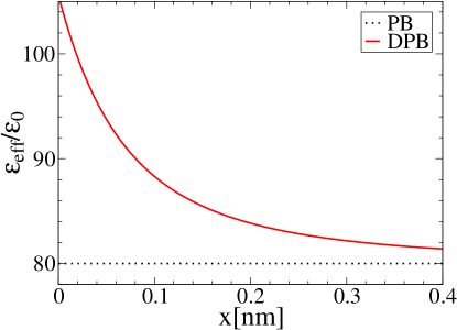
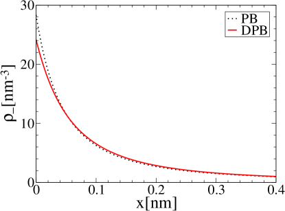
Figure 1: The effective dielectric constant, $\epsilon_{\rm eff}=\epsilon_{0}+p_{0}\rho_{d}{\mathcal{L}}/\psi^{\prime}$, and the counterion density, $\rho_{-}$ (the density of coions is denoted as $\rho_{+}$), for a wall model with surface charge $\sigma_{c}=0.4\,{\rm Cm^{-2}}$. The solvent parameters are: $c_{d}=55\,{\rm M}$ and $p_{0}=4.78\,{\rm D}$, such that in the linear polarization regime the dielectric constant of water is recovered, $\epsilon_{\rm sol}/\epsilon_{0}=1+\beta c_{d}p_{0}^{2}/3\epsilon_{0}=80$. The remaining parameters are $\lambda_{B}=\beta e^{2}/4\pi\epsilon_{\rm sol}=0.72\,{\rm nm}$ and $c_{s}=0.1\,{\rm M}$.

The saturation effect of the Langevin function is, therefore, not dominant. As a consequence, the counterion density is depleted from the wall region. (A dipole in a uniform electrostatic field adjusts its orientation but not is position since there can be no gain in energy. In order to transport dipoles, a nonuniform field is required. This type of transport is referred to as dielectrophoresis. The reason for the concentration gradient of dipoles near a wall in Fig. (1) reflects the fact that a field is nonuniform due to nonuniform distribution of counterions and coions).

The dipolar PB model can be employed for studies of solvent mixtures. Given a mixture of two solvents with different dipole moment, $p_{1}\neq p_{2}$, the solvent with higher polarity will prefer the vicinity of a charged surface, as a more efficient screening medium David09 ; David11 ; David13 . The dipolar PB model captures this behavior as seen in Fig. (2), where the hydration shell at a charged surface is comprised primarily of solvent of higher polarity. A heterogenous hydration shell formed around ions dissolved in a solvent mixture can induce additional, ion-hydration interactions, leading still to other ion-specific effects.

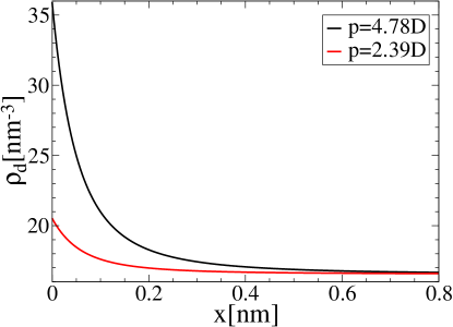
Figure 2: Densities of two dipolar species in a solvent mixture. The same parameters as in Fig. (1), except the solvent parameters are: $c_{d1}=c_{d2}=27.5\,{\rm M}$, and $p_{1}=2p_{2}=4.78\,{\rm D}$.

III.3 Langevin Poisson-Boltzmann equation

In the dipolar PB equation solvent obeys ideal-gas entropy. But as water is not very compressible, a more realistic representation of a solvent should take into account excluded volume interactions. Such interactions have been implemented through a local scheme based on the lattice-gas entropy Birkman42 ; David97 ; Henri08 ; Henri09a ; Henri09b ; Bohinc10 . Here, we make a simple assumption that water is incompressible, and the solvent density is uniform everywhere, $\rho_{d}({\bf r})\to c_{d}$. This reduction leads to the Langevin PB equation, where the polarization density is determined solely by the Langevin function, $P=c_{d}p_{0}{\mathcal{L}}(\beta p_{0}|\mbox{\boldmath$\nabla$}\psi|)$ Frydel11a ; Frydel14 ,

$$\mbox{\boldmath$\nabla$}\cdot\Bigg{[}\Bigg{(}\epsilon_{0}+\frac{c_{d}p_{0}\,{\mathcal{L}}(\beta p_{0}|\mbox{\boldmath$\nabla$}\psi|)}{|\mbox{\boldmath$\nabla$}\psi|}\Bigg{)}\mbox{\boldmath$\nabla$}\psi\Bigg{]}=-\sum_{i=1}^{K}q_{i}c_{i}e^{-\beta q_{i}\psi}.$$ (54)

The effective dielectric constant in parentheses has two limiting behaviors. In the limit $|\mbox{\boldmath$\nabla$}\psi|\to 0$, it is the same as for the dipolar PB equation,

$$\epsilon\to\epsilon_{0}+\frac{\beta c_{d}p_{0}^{2}}{3}=\epsilon_{\rm sol},$$ (55)

but now as $|\mbox{\boldmath$\nabla$}\psi|\to\infty$ and ${\mathcal{L}}\to 1$, the contributions of a solvent to dielectric response vanish,

$$\epsilon\to\epsilon_{0}+\frac{c_{d}p_{0}}{|\mbox{\boldmath$\nabla$}\psi|}$$ (56)

and the nonlinear contributions of the Langevin model lead to dielectric decrement.

Dielectric decrement has been observed for bulk electrolytes, and it reflects structural rearrangement of water due to introduction of salt. For salt concentrations ranging between zero and $1.5\,{\rm M}$, the dielectric constant was found to depend linearly on the salt concentration, $\epsilon_{\rm eff}(c_{s})=\epsilon+\alpha c_{s}$ Collie48 ; David11 ; David12 . The rearrangement of water structure occurs around dissolved ions within the hydration shell. The orientation of these water dipoles is fixed by field lines originating from ion centers, and they cannot respond to an external source of field. This behavior can be quantified with a crude model. As dipoles within the hydration shell are excluded from screening an external electrostatic field, the effective density of free water dipoles becomes reduced, $c_{d}\to c_{d}-(M_{+}c_{+}+M_{-}c_{-})$, where $M_{\pm}$ is the solvation number of water molecules in a hydration shell around either a cation or anion. In the linear regime the dielectric constant of water is $\epsilon=\epsilon_{0}+\beta c_{d}p_{0}^{2}/3$. After addition of salt the effective concentration of salt is $c_{d}\to c_{d}-(M_{+}c_{+}+M_{-}c_{-})$ and the dielectric constant becomes

$$\epsilon\to\epsilon-(c_{+}M_{+}+c_{-}M_{-})\frac{(\epsilon-\epsilon_{0})}{c_{d}}.$$ (57)

In this simple picture $M_{\pm}$ is salt specific.

For the wall model and $1:1$ symmetric electrolyte, the Langevin PB equation becomes,

$$\epsilon_{0}\psi^{\prime\prime}+c_{d}p_{0}{\mathcal{L}}^{\prime}(\beta p_{0}\psi^{\prime})=2ec_{s}\sinh\beta e\psi.$$ (58)

The boundary conditions obtained from the neutrality condition is

$$-\epsilon_{0}\psi^{\prime}_{w}=\sigma_{c}+\sigma_{p},$$ (59)

where

$$\sigma_{p}=c_{d}p_{0}{\mathcal{L}}(\beta p_{0}\psi^{\prime}_{w}),$$ (60)

is the polarization surface charge.

To obtain the contact value theorem, the Langevin PB equation is multiplied by $\psi^{\prime}$,

$$\epsilon_{0}\psi^{\prime}\psi^{\prime\prime}=2ec_{s}\sinh(\beta e\psi)\psi^{\prime}+c_{d}p_{0}{\mathcal{L}}^{\prime}(\beta p_{0}\psi^{\prime})\psi^{\prime},$$ (61)

and after some manipulation we get,

$$\frac{\partial}{\partial x}\big{(}\epsilon_{0}\psi^{\prime 2}\big{)} = \frac{\partial}{\partial x}\big{(}2c_{s}\beta^{-1}\cosh\beta e\psi\big{)}+\frac{\partial}{\partial x}\bigg{(}c_{d}p_{0}{\mathcal{L}}(\beta p_{0}\psi^{\prime})\psi^{\prime}\bigg{)}$$ (62)

$$- \frac{\partial}{\partial x}\bigg{(}c_{d}\beta^{-1}\log\bigg{[}\frac{\sinh\beta p_{0}\psi^{\prime}}{\beta p_{0}\psi^{\prime}}\bigg{]}\bigg{)}.$$

After integration the contact value relation becomes

$$\rho_{w}=\rho_{b}+\frac{\beta}{2\epsilon_{0}}\bigg{(}\sigma_{c}^{2}-\sigma_{p}^{2}\bigg{)}-c_{d}\log\bigg{[}\frac{\sinh[\beta p_{0}(\sigma_{c}+\sigma_{p})/\epsilon_{0}]}{\beta p_{0}(\sigma_{c}+\sigma_{p})/\epsilon_{0}}\bigg{]}.$$ (63)

The results of the Langevin PB equation are shown in Fig. (3). The dielectric constant near a wall decreases as the alignment of dipoles with field lines saturates, ${\mathcal{L}}\to 1$. This is an opposite trend to that found in the dipolar PB equation, which shows dielectric increment, see Fig. (1). The dielectric decrement of the Langevin model generates stronger electrostatic interactions so that counterions stick more tightly to a charged wall.

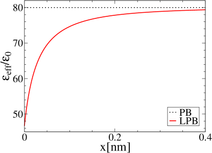
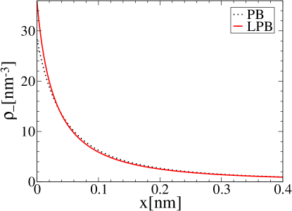
Figure 3: The effective dielectric constant, $\epsilon_{\rm eff}=\epsilon_{0}+p_{0}c_{d}{\mathcal{L}}/\psi^{\prime}$, and the counterion density, $\rho_{-}$ (the density of coins is denoted as $\rho_{+}$) for a wall model and the Langevin PB equation. The same parameters as in Fig. (1), except now the concentration of polar solvent is uniform and fixed at $c_{d}=55\,{\rm M}$.

III.4 Point-dipoles with charge

For the sake of illustration and as a way of transition to polarizable point-charges, we consider point-charges with a dipole moment. The mean-potential that an ion of a species $i$ feels involves two parts,

$$w_{i}({\bf r},\theta)=q_{i}\psi-p_{i}|\mbox{\boldmath$\nabla$}\psi|\cos\theta.$$ (64)

The corresponding mean-field distribution is

$$\varrho_{i}({\bf r},\theta_{i})\sim c_{i}e^{-\beta(q_{i}\psi-p_{i}|\mbox{\boldmath$\nabla$}\psi|\cos\theta_{i})}.$$ (65)

After integrating out the orientational degrees of freedom we arrive at the usual number density,

$$\rho_{i}({\bf r}) = \frac{c_{i}e^{-\beta q_{i}\psi}\epsilon_{\rm sol}\sinh\beta p_{i}|\mbox{\boldmath$\nabla$}\psi|}{\beta p_{i}|\mbox{\boldmath$\nabla$}\psi|}.$$ (66)

Before considering the polarization density we note that in the present model polarization density is associated with the density of ions. In the Langevin model ions and dipoles were separate species. Following Eq. (42) we get

$${\bf P} = \bigg{(}\frac{\mbox{\boldmath$\nabla$}\psi}{|\mbox{\boldmath$\nabla$}\psi|}\bigg{)}\sum_{i=1}^{K}\frac{p_{i}c_{i}e^{-\beta q_{i}\psi}\sinh\beta p_{i}|\mbox{\boldmath$\nabla$}\psi|}{\beta p_{i}|\mbox{\boldmath$\nabla$}\psi|}{\mathcal{L}}(\beta p_{i}|\mbox{\boldmath$\nabla$}\psi|),$$ (67)

and the mean-field Poisson equation becomes

$$\mbox{\boldmath$\nabla$}\cdot\Bigg{[}\Bigg{(}\epsilon + \sum_{i=1}^{K}\frac{p_{i}c_{i}e^{-\beta q_{i}\psi}\sinh\beta p_{i}|\mbox{\boldmath$\nabla$}\psi|}{\beta p_{i}|\mbox{\boldmath$\nabla$}\psi|^{2}}{\mathcal{L}}(\beta p_{i}|\mbox{\boldmath$\nabla$}\psi|)\Bigg{)}\mbox{\boldmath$\nabla$}\psi\Bigg{]}$$ (68)

$$= -\sum_{i=1}^{K}\frac{c_{i}q_{i}e^{-\beta q_{i}\psi}\sinh\beta p_{i}|\mbox{\boldmath$\nabla$}\psi|}{\beta p_{i}|\mbox{\boldmath$\nabla$}\psi|}.$$

Here ions themselves contribute to the dielectric response of the medium on account of their inherent dipole moment. This leads to dielectric increment of a solution medium. Ions with permanent dipole moment are not common. The typical ions such as Cl^- and Na⁺ have spherical distributions. Ions with permanent dipole are encountered in ionic liquids, where ions tend to be larger molecular structures.

III.5 Polarizable Poisson-Boltzmann equation

A dipole moment of a polarizable ion is not permanent but is induced by an external electrostatic field according to the linear relation

$${\bf p}=\alpha{\bf E},$$ (69)

where $\alpha$ is the ion specific polarizability. Polarizability measures elasticity of an electron cloud of a molecule. The larger the electron cloud, the more deformable is the cloud. This behavior is manifest in the sequence for halide ions: ${\rm F}^{-}<{\rm Cl}^{-}<{\rm Br}^{-}<{\rm I}^{-}$.

Polarizability is in fact a more general concept and measures response of an electron cloud to a time dependent field leading to a frequency dependent polarizability. Our strict concern is with static, or zero-frequency polarizability as variations of an electric field induced by thermal fluctuations of an electrolyte operate at timescales much larger than timescales of inner dynamics of an electron cloud. Frequency dependent polarizability can lead to other effects, such as the London forces London37 when fluctuations in electron cloud of two nearby molecules become synchronized. These, however, are less important than the ion-dipole interactions generated by static polarizability Netz04a ; Netz04b .

Polarizability can be treated by recourse to a harmonic oscillator model, where opposite charges can be displaced relative to one another under the action of an applied electric field, and the resorting force is proportional to a displacement and the stiffness parameter $k$. The mean-potential for a species $i$ is then written as

$$w_{i}({\bf r})=q_{i}\psi-p_{i}|\mbox{\boldmath$\nabla$}\psi|+\frac{k_{i}}{2}d_{i}^{2},$$ (70)

where the last two terms characterize the energy of an induced dipole. The electrostatic energy of a dipole is always in alignment with a field, and there is no orientational degree of freedom as for the case of a permanent dipole. The last term is the energy of a harmonic oscillator. To relate the stiffness parameter $k$ to the polarizability $\alpha$ we start with the Hooke’s law, ${\bf F}=k{\bf d}$, where the stretching force is electrostatic, ${\bf F}={q\bf E}$, and a dipole moment is related to a displacement, ${\bf p}=q{\bf d}$ ($q$ is the charge of the two charges being pulled apart). Substituting these definitions into the Hooke’s law we get

$${\bf p}=\bigg{(}\frac{q^{2}}{k}\bigg{)}{\bf E},$$ (71)

so that from Eq. (69) we get

$$k=\frac{q^{2}}{\alpha}.$$ (72)

The mean-potential in Eq. (70) can now be written as,

$$w_{i}({\bf r})=q_{i}\psi-\frac{\alpha_{i}}{2}|\mbox{\boldmath$\nabla$}\psi|^{2},$$ (73)

and the mean-field density becomes

$$\rho_{i}({\bf r})=c_{i}e^{-\beta(q_{i}\psi-\alpha_{i}|\mbox{\boldmath$\nabla$}\psi|^{2}/2)},$$ (74)

leading to the following polarization density,

$${\bf P}=-\mbox{\boldmath$\nabla$}\psi\Bigg{(}\sum_{i=1}^{K}\alpha_{i}c_{i}e^{-\beta(q_{i}\psi-\alpha_{i}|\mbox{\boldmath$\nabla$}\psi|^{2}/2)}\Bigg{)}.$$ (75)

Polarization no longer depends on the Langevin function as it did for ions with a permanent dipole moment. All nonlinearity of the expression is linked to the local ion density. The polarizable PB equation that results is Outhwaite89 ; Frydel11b

$$\mbox{\boldmath$\nabla$}\cdot\Bigg{[}\Bigg{(}\epsilon+\sum_{i=1}^{K}\alpha_{i}c_{i}e^{-\beta(q_{i}\psi-\alpha_{i}|\mbox{\boldmath$\nabla$}\psi|^{2}/2)}\Bigg{)}\mbox{\boldmath$\nabla$}\psi\Bigg{]}=\sum_{i=1}^{K}q_{i}c_{i}e^{-\beta(q_{i}\psi-\alpha_{i}|\mbox{\boldmath$\nabla$}\psi|^{2}/2)}$$ (76)

For a wall model and a symmetric $1:1$ electrolyte, where all ions have the same polarizability $\alpha$, the polarizable PB equation becomes

$$\epsilon\psi^{\prime\prime}+\frac{\partial}{\partial x}\Big{[}2\alpha c_{s}\psi^{\prime}\cosh(\beta e\psi)e^{\beta\alpha\psi^{\prime 2}/2}\Big{]}=2ec_{s}\sinh(\beta e\psi)e^{\beta\alpha\psi^{\prime 2}/2}.$$ (77)

The boundary conditions at the wall are

$$-\epsilon\psi^{\prime}_{w}=\sigma_{c}+\sigma_{p},$$ (78)

where the polarization surface charge is

$$\sigma_{p}=2\alpha c_{s}\psi^{\prime}_{w}\cosh(\beta e\psi_{w})e^{\beta\alpha\psi^{\prime 2}_{w}/2}.$$ (79)

Finally, the contact value theorem for the present model is

$$\rho_{w}=\rho_{b}+\frac{\beta}{2\epsilon}\Big{(}\sigma_{c}^{2}-\sigma_{p}^{2}\Big{)},$$ (80)

obtained according to the procedure in Eq. (61). Equations (78), (79), and (80) can be combined to yield a single equation for either $\rho_{w}$ or $\sigma_{p}$. Below we write down the equation for the ratio $\sigma_{p}/\sigma_{c}$, which can be considered as a measure of polarizability,

$$\bigg{(}\frac{\sigma_{p}}{\sigma_{c}}\bigg{)}^{3}+\bigg{(}\frac{\sigma_{p}}{\sigma_{c}}\bigg{)}^{2}-\Bigg{(}1+\frac{2\epsilon\rho_{b}}{\beta\sigma_{c}^{2}}+\frac{2\epsilon^{2}}{\beta\alpha\sigma_{c}^{2}}\Bigg{)}\bigg{(}\frac{\sigma_{p}}{\sigma_{c}}\bigg{)}-\Bigg{(}1+\frac{2\epsilon\rho_{b}}{\beta\sigma_{c}^{2}}\Bigg{)}=0.$$ (81)

$\sigma_{p}/\sigma_{c}$ spans the range $[0,-1)$ as $\alpha$ increases. $\sigma_{p}/\sigma_{c}=-1$ indicates that $\sigma_{p}$ cancels out the bare surface charge. From the cubic equation above we obtain the dimensionless polarizability parameter,

$$\alpha^{*}=\bigg{(}\frac{\beta\sigma_{c}^{2}\alpha}{2\epsilon^{2}}\bigg{)},$$

that controls the polarizability contributions at a charged surface. The other parameter, $\frac{2\epsilon\rho_{b}}{\beta\sigma_{c}^{2}}$, depends on a salt concentration.

If we take an electrolyte at room temperature, the surface charge $\sigma_{c}=0.4\,{\rm Cm^{-2}}$, and the polarizability $\alpha/(4\pi\epsilon_{0})=10\,{\rm\AA}^{3}$, then the dimensionless polarizability parameter is $\alpha^{*}\approx 0.04$. Polarizability $\alpha/(4\pi\epsilon_{0})=10\,{\rm\AA}^{3}$ corresponds roughly with the polarizability of iodide ion I^- and is already rather high. We conclude then that polarizability of typical salts has small effect on electrolytes.

Polarizability contributions can be increased for dielectric media with low dielectric constant. Such a situation is realized in ionic liquids, where the absence of a polar solvent permits unscreened electrostatic interactions, as ionic liquids are melted salts. In Fig. (4) we consider an electrolyte with reduced dielectric constant, $\epsilon/\epsilon_{0}=10$ (which yields a larger Bjerrum length, $\lambda_{B}=5.76\,{\rm nm}$).

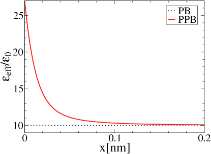
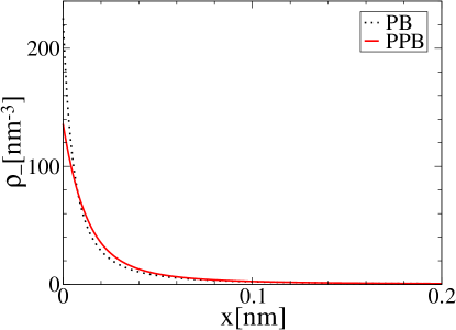
Figure 4: Effective dielectric constant $\epsilon_{\rm eff}=\epsilon+2\alpha c_{s}\cosh\beta e\psi$, and the counterion density profile for reduced dielectric constant, $\epsilon/\epsilon_{0}=10$ (in water $\epsilon/\epsilon_{0}=80$). The relevant system parameters are: $\sigma_{c}=0.4\,{\rm Cm^{-2}}$, $\lambda_{B}=5.76\,{\rm nm}$, $c_{s}=0.1\,{\rm M}$, and $\alpha/(4\pi\epsilon_{0})=10{\rm\AA}^{3}$.

The increased dielectric constant near a wall region, which reflects a counterion profile, $\epsilon_{\rm eff}=\epsilon+2\alpha c_{s}\cosh\beta e\psi$, generates a weaker attraction to a surface charge, so that counterions become more spread out.

The present model can by applied to study of ion specificity by assigning different polarizabilities to ion species. In Fig. (5) we show density profiles for counterions with the same charge but different polarizability, $\alpha_{1}/(4\pi\epsilon_{0})=0{\rm\AA}^{3}$ and $\alpha_{2}/(4\pi\epsilon_{0})=10{\rm\AA}^{3}$. Polarizable counterions being a better screening agent are preferred near a wall.

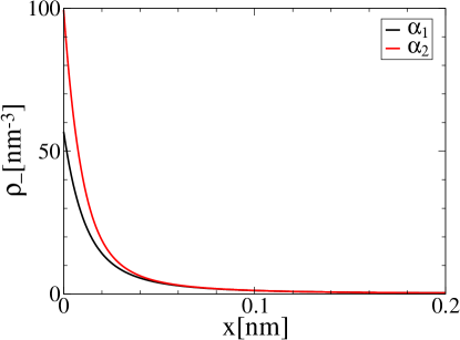
Figure 5: The counterion profiles for polarizable and non-polarizable ions. The same parameters as in Fig. (4) but now only half of the ions are polarizable: $\alpha_{1}=0{\rm\AA}^{3}$ and $\alpha_{2}=10{\rm\AA}^{3}$.

III.5.1 Negative Excess polarizability

The present mean-field framework developed for polarizable ions has been used to capture the physics of dielectric decrement caused by the restructuring of water as hydration shells form around dissolved ions Hatlo12 ; Rudi12 . Since polarizable ions in general cause dielectric increment, dielectric decrement can easily be realized when using negative values of polarizability. Negative polarizability occurs in quantum mechanics for molecules in excited state or for non-static polarizabilities, but in soft-matter it is an effective phenomena. Negative polarizability means that induced dipole acts opposite to the local field. This conceptually captures the fact that the water dipoles in a hydration shell do not respond to electrostatic field.

According to Eq. (57), the dielectric increment/decrement depends linearly on the salt concentration. The same linear dependence is found for the polarizable PB model,

$$\epsilon_{\rm eff}-\epsilon=\alpha_{+}\rho_{+}+\alpha_{-}\rho_{-},$$ (82)

where, after comparing with Eq. (57), the negative excess polarizability can be approximated as

$$\alpha_{\pm}=-M_{\pm}\bigg{(}\frac{\epsilon-\epsilon_{0}}{c_{d}}\bigg{)}.$$ (83)

Even for a modest value of a solvation number, $M_{\pm}=4$, the excess polarizability is already significant, $\alpha/(4\pi\epsilon_{0})\approx-300{\rm\AA}^{3}$, where we assume $M_{+}=M_{-}=M$ and $\alpha_{+}=\alpha_{-}=\alpha$.

In Fig. (6) we show the results for $\alpha/(4\pi\epsilon_{0})=-300{\rm\AA}^{3}$. We compare the plots with positive polarizability of the same magnitude, $\alpha/(4\pi\epsilon_{0})=300{\rm\AA}^{3}$. The negative polarizability, as expected, lowers the dielectric constant near a wall. Less intuitive is the fact that this leads to depletion of counterions from the wall region. The depletion is, furthermore, more significant than that for positive polarizability. If the electrostatic screening is reduced in the wall region than counterions should hug to the wall more tightly. This is, at least, what we see in Fig. (3) for the Langevin PB model. So why does the Langevin PB model satisfies our intuitions and the polarizable PB model for negative polarizabilities does not? Formal answer to this puzzle can be found by examining the contact value theorem in Eq. (80). The sign of the polarization surface charge, $\sigma_{p}$, does not matter, and any polarizability lowers the contact density, $\rho_{w}$.

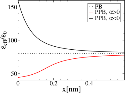
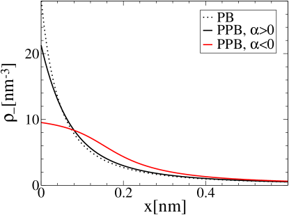
Figure 6: Effective dielectric constant $\epsilon_{\rm eff}=\epsilon+2\alpha c_{s}\cosh\beta e\psi$, and the counterion density profile for negative excess polarizability $\alpha/(4\pi\epsilon_{0})=-300{\rm\AA}^{3}$. The dielectric constant of a solvent background is that of water, $\epsilon/\epsilon_{0}=80$. The remaining parameters are: $\sigma_{c}=0.4\,{\rm Cm^{-2}}$, $\lambda_{B}=0.72\,{\rm nm}$, $c_{s}=0.1\,{\rm M}$.

The two models, the Langevin and the polarizable PB equation with $\alpha<0$ are designed to represent the same phenomena, the lowering of a dielectric constant as the hydration structures form around dissolved ions. The results, however, are not precisely comparable. Decrement of a dielectric constant near a wall are captured by both models, but density profiles are not comparable, even qualitatively. Counterion profiles of the Langevin model are more concentrated, while those of the polarizable model are more dilute. Without exact simulation results, it is hard to know which model is accurate. In recent work by Ma et al. Zhenli14 the Langevin PB equation with correlations has been solved and it yields a non-monotonic density profile with a valey at a wall followed by a peak further away from a wall. The depletion is, therefore, captured but immediately at a wall and not for the entire profile. A possible weak point of the negative polarizability model is the linearity assumption, $\epsilon_{\rm eff}-\epsilon\sim-c_{s}$. For homogenous solutions linearity breaks down for higher concentrations David13 , as hydration shells begin to overlap. This suggests that near a wall, where concentrations are high, this too could have its effect.

IV Finite-Spread Poisson-Boltzmann Equation

An alternative approach to introduce structure of a charged particle is to smear its net charge within a finite volume according to a desired distribution $\omega({\bf r}-{\bf r}_{0})$ such that

$$q=\int d{\bf r}\,\omega({\bf r}-{\bf r}_{0}).$$ (84)

An arbitrary distribution is expected to depend on, in addition to the position ${\bf r}_{0}$, the orientation characterized by three angles. An arbitrary distribution embodies dipole,

$${\bf p}=\int d{\bf r}\,({\bf r}-{\bf r}_{0})\omega({\bf r}-{\bf r}_{0}),$$ (85)

and higher order multipoles. If the two distributions at ${\bf r}_{i}$ and ${\bf r}_{j}$, do not overlap, there is no difference between the finite-spread and point-ion representation. The difference occurs for overlapping separations and the resulting potential,

$$U({\bf r}_{i}-{\bf r}_{j})=\int d{\bf r}\int d{\bf r}^{\prime}\,\frac{\omega({\bf r}-{\bf r}_{i})\omega({\bf r}^{\prime}-{\bf r}_{j})}{4\pi\epsilon|{\bf r}-{\bf r}^{\prime}|},$$ (86)

is no longer described as a truncated series of multipoles.

The finite-spread model does not want to provide a detailed electronic structure of an ion. This is beyond the scope of classical physics. But there are particles whose charge distribution is better described as extended in space, rather than as a sequence of multipoles. Among examples are charged rods, dumbbell shaped particles Pincus08 ; Bohinc08 ; Bohinc11 ; Bohinc12 , or macromolecules whose non-electrostatic interactions are ”ultrasoft”, allowing interpenetration, and the distribution of charge in space is a sensible representation Likos01 . A perfect example is a polyelectrolyte in a good solvent whose charges along a polymer chain appear on average as a smeared-out cloud due to quickly alternating configurations. Uncharged, two chain polymers interact via a Gaussian potential representing steric interactions of two self-avoiding polymer chains Hansen00a . Dendrimers offer another example of a soft, flexible macromolecule Likos01a .

There is also a more fundamental aspect of smeared-out charges: a smear-out point-charge is rid of divergence. For same-charged ions this eliminates effective excluded volume effects of a Coulomb potential and permits interpenetration of two or more charges. For opposite-charged ions it leads to a new type of a Bjerrum pair where two ions collapse into a neutral but polarizable entity Hansen11a ; Hansen11b ; Hansen12 ; Warren13 . The usual Bjerrum pair, formed between ions with hard-core interactions, is represented as a permanent dipole Yan93 .

Ultrasoft repulsive interactions (without the long-range Coulomb part) have been extensively studied, both for its theoretical aspects and as a description of a soft matter system. Studies reveal two distinct behaviors. Some ultrasoft potentials supports ”stacked” configurations, where two or more particles collapse, even though no true attractive interactions come into play Lowen01 ; Likos06 . This behavior leads to a peak in a correlation function around $r=0$. To this class of potentials belongs the penetrable sphere model Witten89 . The Gaussian core model Stillinger76 , on the other hand, represents the class of sort particles unable to support stacked configurations.

As a note of interest, we mention that the interest in ultrasoft interactions is not confined to soft-matter. The soft-core boson model with interactions $U(r)\sim(R^{6}+r^{6})^{-1}$, where $R$ is the soft-core radius, has been studied in Pohl14 in connection to superfluidity. By removing the singularity from the potential, boson particles cluster and form crystal with multiple particles occupying the same lattice sites.

IV.1 Spherical Distribution $\omega(|{\bf r}-{\bf r}_{0}|)$

In this section we consider ion species with spherically symmetric distribution $\omega_{i}(|{\bf r}-{\bf r}_{0}|)$. As in previous mean-field constructions, we start with the mean-potential that an ion of the species $i$ feels,

$$w_{i}({\bf r})=\int d{\bf r}^{\prime}\,\omega_{i}(|{\bf r}-{\bf r}^{\prime}|)\psi({\bf r}^{\prime}).$$ (87)

The non-locality of the expression reflects the finite distribution of an ion charge in space and the fact that every part of this distribution interacts with an electrostatic field. The number density that follows is

$$\rho_{i}({\bf r})=c_{i}e^{-\beta\int d{\bf r}^{\prime}\,\omega_{i}(|{\bf r}-{\bf r}^{\prime}|)\psi({\bf r}^{\prime})}.$$ (88)

To obtain the appropriate PB equation we need an expression for the charge density, which is given as the convolution of the number density,

$$\rho_{c}({\bf r})=\sum_{i=1}^{K}\int d{\bf r}^{\prime}\,\omega_{i}(|{\bf r}-{\bf r}^{\prime}|)\rho_{i}({\bf r}^{\prime}).$$ (89)

Convolution is, again, a result of the finite extension of a charge. Using an explicit expression for $\rho_{i}$ we get

$$\rho_{c}({\bf r})=\sum_{i=1}^{K}c_{i}\int d{\bf r}^{\prime}\,\omega_{i}({\bf r}-{\bf r}^{\prime})e^{-\beta\int d{\bf r}^{\prime\prime}\,\omega_{i}({\bf r}^{\prime}-{\bf r}^{\prime\prime})\psi({\bf r}^{\prime\prime})},$$ (90)

and the finite-spread PB equation for smeared-out ions is Frydel13

$$\epsilon\nabla^{2}\psi=-\sum_{i=1}^{K}c_{i}\int d{\bf r}^{\prime}\,\omega_{i}(|{\bf r}-{\bf r}^{\prime}|)e^{-\beta\int d{\bf r}^{\prime\prime}\,\omega_{i}(|{\bf r}^{\prime}-{\bf r}^{\prime\prime}|)\psi({\bf r}^{\prime\prime})}.$$ (91)

To complete the model, we still need to choose a specific spherical distribution. We model ions as uniformly distributed charges within a spherical volume,

$$\omega_{i}(|{\bf r}-{\bf r}^{\prime}|)=\frac{3q_{i}}{4\pi R_{i}^{3}}\theta(R_{i}-|{\bf r}-{\bf r}^{\prime}|),$$ (92)

where $q_{i}$ and $R_{i}$ are the charge and the radius of an ion species $i$, respectively. The pair interaction between two ions with charge $q$ and size $R$, when the two ions overlap, is

$$U(r\leq 2R)=\frac{q^{2}}{4\pi\epsilon R}\Bigg{[}\frac{6}{5}-\frac{1}{2}\Big{(}\frac{r}{R}\Big{)}^{2}+\frac{3}{16}\Big{(}\frac{r}{R}\Big{)}^{3}-\frac{1}{160}\Big{(}\frac{r}{R}\Big{)}^{5}\Bigg{]},$$ (93)

when not overlapping the usual Coulomb potential is recovered,

$$U(r>2R)=\frac{q^{2}}{4\pi\epsilon R}\Big{(}\frac{r}{R}\Big{)}^{-1}.$$ (94)

If overlap is complete the pair interaction remains finite,

$$U(0)=\frac{6}{5}\frac{q^{2}}{4\pi\epsilon R},$$ (95)

and is said to be bounded. In Fig. (7) we plot various realizations of the pair potential $U(r)$ for different ion size $R$. The degree of penetration clearly increases with increasing $R$.

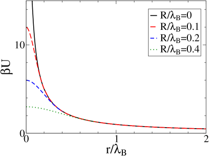
Figure 7: Pair potential between two charge distributions in Eq. (92) for different $R$. At overlapping separations the functional form of a pair potential is that in Eq. (93).

The mean-field Poisson equation for a symmetric $1:1$ electrolyte, with ion distributions in Eq. (92), is

$$\epsilon\nabla^{2}\psi = \frac{6ec_{s}}{4\pi R^{3}}\int d{\bf r}^{\prime}\,\theta(R-|{\bf r}-{\bf r}^{\prime}|)$$

$$\times \sinh\bigg{[}{-\frac{3\beta e}{4\pi R^{3}}\int d{\bf r}^{\prime\prime}\,\theta(R-|{\bf r}^{\prime}-{\bf r}^{\prime\prime}|)\psi({\bf r}^{\prime\prime})}\bigg{]}.$$

For the wall model we the integral terms simplify,

$$\int d{\bf r}^{\prime}\,\theta(R-|{\bf r}-{\bf r}^{\prime}|)f(z)=\pi\int_{-R}^{R}dz^{\prime}\,f(z+z^{\prime})(R^{2}-z^{\prime 2}),$$ (97)

where for $f(z)=1$ we recover $4\pi R^{3}/3$, a volume of a sphere. And the finite-spread PB equation becomes

$$\epsilon\psi^{\prime\prime}=\frac{6ec_{s}}{4R^{3}}\int_{-R}^{R}dz^{\prime}\,(R^{2}-z^{\prime 2})\sinh\bigg{[}{-\frac{3\beta e}{4R^{3}}\int_{-R}^{R}dz^{\prime\prime}\,\psi(z+z^{\prime}+z^{\prime\prime})(R^{2}-z^{\prime\prime 2})}\bigg{]}.$$ (98)

For the wall model particle centers are confined to the half-space $x>0$ but a charge density starts from $x>-R$ due to finite size of an ionic charge as half of a sphere sticks out. The boundary conditions, therefore, are not determined at the wall, $x=0$, but at $x=-R$,

$$-\epsilon\psi^{\prime}(-R)=\sigma_{c}.$$ (99)

This implies that the surface charge is at $x=-R$. The contact value theorem, however, is not effected and is the same as for the standard PB equation,

$$\rho_{w}=\rho_{b}+\frac{\beta\sigma_{c}^{2}}{2\epsilon},$$ (100)

where $\rho_{w}=\rho(0)$.

In Fig. (8) we plot electrostatic quantities of penetrable ions: a charge density and an electrostatic potential. Unlike the number density, these quantities are not confined to the region $x>0$, and extend to $x=-R$ as the charge of an ion sticks out. Note how the sharp peak in the charge density for the standard PB model is smoothed-out in the finite-spread model.

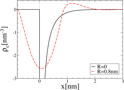
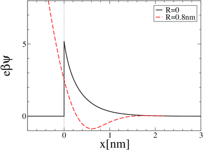
Figure 8: The charge density and electrostatic potential for penetrable ions with charge distribution in Eq. (92) with $R=0.8\,{\rm nm}$. The ion centers are confined to the half-space $x>0$ and the vertical line at $x=0$ marks the half-space available to ion centers. The results for $R=0$ correspond to those for the standard PB equation. The system parameters are $\sigma_{c}=0.4\,{\rm C/m^{2}}$, $\lambda_{B}=0.72\,{\rm nm}$, and $c_{s}=1\,{\rm M}$.

Fig. (9) shows number density profiles for penetrable ions. The first striking feature is that profiles are non-monotonic. More surprising still is the fact that a surface charged is overcharged: more counterions accumulate at a wall than needed for neutralizing it. Overcharging is signaled by a peak in coion density and indicates attraction of coions to a same-charged surface. Attraction between same-charged plates was found for dumbbell shaped counterions in Pincus08 , suggesting that charge inversion is a common feature of charges extended in space.

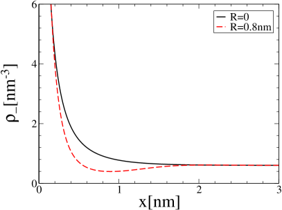
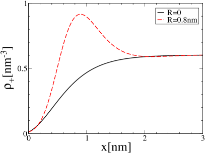
Figure 9: The number density profiles for counter- and co-ions for penetrable ions near a charged wall. The same parameters as in Fig. (8).

A closer look into plots reveals that overcharging and consequent charge inversion is a more complex phenomenon. To magnify these features we plot in Fig. (10) the number densities for a symmetric $3:3$ electrolyte. What we see is not a simple charge inversion but rather an alternating layers of counterions and coions leading to oscillations in density profiles. This behavior is reminiscent of polyelectrolyte layer-by-layer adsorption onto a charged substrate Borukhov98 ; Polylayer05 ; Polylayer10 .

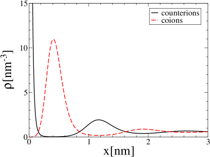
Figure 10: Number density profiles for counterions and coions with valance number $3$. The increased electrostatic interactions magnify the features in Fig. (9). Otherwise the same parameters as those in Fig. (8).

In Fig. (11) we show Monte Carlo snapshots for counterions adsorbed onto a charged wall. The figure compares two systems: counterions that approximate a point-charges with size $R=0.1\,{\rm nm}$, and counterions that are fully penetrable with size $R=0.8\,{\rm nm}$. A configuration for smaller ions appears more or less evenly distributed, indicating the strong presence of correlations, although the structure is still far from the Wigner crystal Trizac11 . There is no overcharging observed for this system, although deviations from the mean-field are sufficiently significant to yield counterion density profiles different than those of the standard PB equation by being shifted closer to a wall. On the other hand, the configuration for $R=0.8\,{\rm nm}$ is more arbitrary and there are numerous overlaps. In this system counterions are in excess and overcharge the surface charge. Furthermore, the correlations have no part in the overcharging mechanism as the Monte Carlo and the finite-spread PB equation yield identical profiles, see Fig. (12).

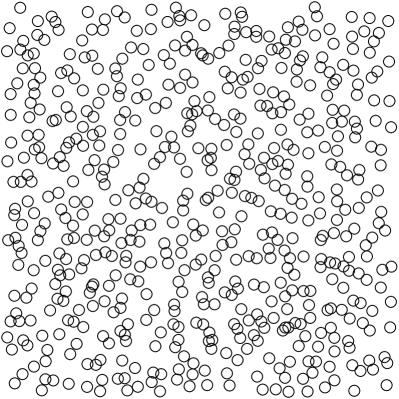
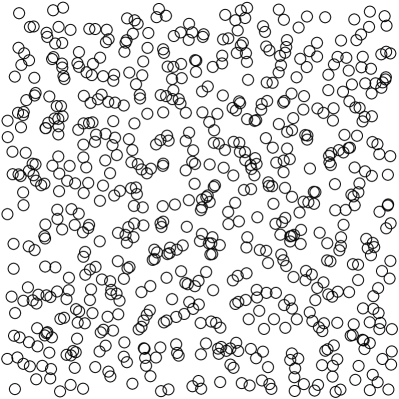
Figure 11: Monte Carlo configuration snapshots for counterions adsorbed onto a charged wall (within the slice $0<x<0.35\,{\rm nm}$). The conditions are the same as for results in Fig. (12). The circles representing particles have diameter $\sigma=0.5\,{\rm nm}$ and are selected arbitrarily for visualization. The first snapshot is for $R=0.1\,{\rm nm}$, essential non-penetrable ions, and the second snapshot is for $R=0.8\,{\rm nm}$, the fully penetrable ions. The 2D densities of each snapshot are $\rho_{2d}=2.34{\rm nm^{-2}}$ and $\rho_{2d}=2.68{\rm nm^{-2}}$, respectively. For comparison, the surface charge density is $\sigma_{c}/e=2.50\,{\rm nm^{-2}}$, indicating overcharging for $R=0.8\,{\rm nm}$ counterions.

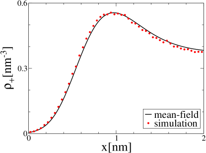
Figure 12: The coion density profile near a charged wall. The mean-field theory very accurately reproduces the exact results of the Monte Carlo simulation. The number of particles in the simulation box is $N_{+}=N_{-}=1200$, and the box size is $L_{y}=L_{z}=16{\rm nm}$ and $L_{x}=12{\rm nm}$. The periodic boundary conditions are in the lateral $(y,z)$-directions. The other parameters are: $\lambda_{B}=0.72\,{\rm nm}$, $R=0.8\,{\rm nm}$, and $\sigma_{c}=0.4\,{\rm Cm^{-2}}$.

The agreement between the mean-field profiles and those from the Monte Carlo simulation rules out correlations as being behind the observed charge inversion. The mechanism must then come from other quarters. According to an orthodox charge inversion mechanism, driven by correlations, adsorbed onto a charged wall counterions come close to form a Wigner crystal, at least locally if not globally Yan02 ; Shklovskii02 . High degree of ordering leads to irregularities in the potential landscape of a now neutralized surface at distances smaller or comparable to the lattice size. These irregularities have attractive spots which can accommodate an additional counterion. For penetrable ions the absence of correlations makes this picture obsolete. What drives overcharging is the low energy cost for overlapping configurations. This energy cost in inversely proportional to the radius $R$, see Eq. (93). By taking the limit $R\to\infty$ we recover the ideal gas limit. A divergence in the pair interactions for point-ions acts as an effective hard-shpere interaction whose radius depends on the Bjerrum length as well as a surface charge. This leads to the effective excluded volume interactions. By removing a divergence and permitting interpenetration, the effective excluded volume interactions are eliminated. This completely changes the lateral structure of adsorbed counterions.

IV.1.1 stacked configurations

A configuration snapshot for penetrable ions in Fig. (11) gives impression that counterions form stacked configurations, detected from the correlation function by the presence of a peak around $r=0$. The presence of stacked formations is, furthermore, linked to instability of the Kirkwood analysis Klein77b ; Klein77a ; Klein80 ; Frisch69 ; Nagai74 . The Kirkwood analysis is the mean-field type of an analysis. As already said in section II, even though the mean-field approximation does not incorporate explicit correlations in its free energy formulation, the correlations can be extracted using exact thermodynamic relations. This is possible because the mean-field is not a self-consistent approximation. Thus, the exact relation in Eq. (12) yields Eq. (14) from the mean-field density, which then can be put in the form of the Ornstein-Zernike equation, as done in Eq. (15), which, when Fourier transformed, becomes,

$$h(k)=-\frac{\beta u(k)}{1+\rho\beta u(k)},$$ (101)

and the corresponding structure factor, defined as $S(k)=1+\rho h(k)$, is

$$S(k)=\frac{1}{1+\rho\beta u(k)}.$$ (102)

All is good as long as $u(k)$ is a non-negative function. But if for some modes $k$ the Fourier transformed pair potential is negative, $S(k)$ becomes divergent for some wave number $k_{0}$, indicating divergent fluctuations. In addition, the onset of this so-called Kirkwood instability coincides with an onset of the long-range correlation order and with a bifurcation point where a constant density no longer yields minimum free energy and another periodic solution takes precedence Klein77b . The instability was later linked to the spinodal of the supercooled liquid.

Simulations of the penetrable sphere model (exhibiting the Kirkwood instability) showed the existence of stacked configurations (referred to as ”clumps” in that work) at temperatures below instability Klein94 . Individual stacks arranged into crystal structure (corresponding to the global minimum) or amorphous glassy structures (corresponding to a local minimum). Stacked structures gave rise to a peak around $r=0$ in the correlation function. A more thorough analysis supported by simulations linked the instability to crystals with multiply occupied lattice sites Lowen98 ; Schmidt99 ; Lowen01 . Potentials whose Fourier transformed potential $u(k)$ is positive remain always stable and are not found to form stacked crystal formations. Instead their solid phase exhibits reentrant melting upon squeezing, a behavior seen in water Stillinger97 .

In the present work we are interested in the liquid structure before the onset of instability. In particular, we want to know if the penetrable ions exhibit Kirkwood instability linked to stacked formations, and if yes, what role they play in a charge inversion mechanism.

It is enough to consider the one component plasma of penetrable ions. The Fourier transformed pair potential depends on the distribution $\omega$ and is obtained from Eq. (86),

$$U(k)=\frac{\omega^{2}(k)}{\epsilon k^{2}}.$$ (103)

For point-ions $\omega(k)=q$, and for penetrable ions $\lim_{k\to 0}\omega(k)=q$, since at large separations the usual Coulomb interactions are recovered. The difference between point and spread-out ions is seen for large $k$, where $S(k)$ reflects behavior for small separations. Regardless of the distribution $\omega(k)$, $U(k)\geq 0$ for any $k$ and the Kirkwood instability does not occur. Stacked formations, therefore, can be excluded as playing any part in a mechanism for charge inversion.

It is not clear, however, whether the conclusion holds for all Coulomb potentials with soft-core, or if it is specific to smeared-out ions. To address this concern, we consider the following soft-core Coulomb potential,

$$u(r)=\begin{cases}\frac{q^{2}}{4\pi\epsilon r}&\text{if }r\geq\sigma\\ \frac{q^{2}}{4\pi\epsilon\sigma}&\text{if }r<\sigma,\end{cases}$$ (104)

whose Fourier transform is

$$u(k)=\frac{q^{2}}{\epsilon k^{2}}\frac{\sin k\sigma}{k\sigma}.$$ (105)

$U(k)$ is no longer a non-negative function and yields instability in the mean-field structure factor. The mean-field correlation function, furthermore, shows a peak at $r=0$,

$$h(0)=-\frac{1}{2\pi^{2}}\int_{0}^{\infty}dk\,\frac{\beta U(k)k^{2}}{1+\rho\beta u(k)},$$ (106)

under certain conditions. We conclude that while the smearing-out procedure cannot lead to Kirkwood instability, this behavior is not general to all Coulomb potentials with soft-core.

.

IV.2 Needle-ions: the case for non-spherical $\omega({\bf r}-{\bf r}^{\prime})$

The modified PB equation for non-spherical distributions is more complicated as there are three additional degrees of freedom for a particle orientation to cope with. Levy et al. David13 derived the modified PB equation for a general distribution using the field-theory methodology.

In this section we consider, as an example of non-spherical distribution, needle-ions. We perform our construction as before, by writing down a mean-potential from which we obtain a number and charge densities. A needle-ion consists of a charge $q$ uniformly distributed along a line of length $d$. The charge distribution of a needle-ion is

$$\omega({\bf r}-{\bf r}_{0},{\bf n})=\frac{q}{d}\int_{-d/2}^{d/2}ds\,\delta({\bf r}_{0}+s{\bf n}-{\bf r}),$$ (107)

where ${\bf r}_{0}$ is a midpoint and ${\bf n}$ is a unit vector that designates orientation. The mean-potential that a needle-ion of a species $i$ feels when its center is at ${\bf r}$ is

$$w_{i}({\bf r},{\bf n})=\frac{q_{i}}{d_{i}}\int d{\bf r}^{\prime}\,\psi({\bf r}^{\prime})\int_{-d_{i}/2}^{d_{i}/2}ds\,\delta({\bf r}+s{\bf n}-{\bf r}^{\prime}),$$ (108)

or, suppressing the delta function, we may alternatively write

$$w_{i}({\bf r},{\bf n})=\frac{q_{i}}{d_{i}}\int_{-d_{i}/2}^{d_{i}/2}ds\,\psi({\bf r}+s{\bf n}).$$ (109)

A nonlocal contribution comes from particle’s finite extension in space. The mean-field expression for the number density in space and orientation is

$$\varrho_{i}({\bf r},{\bf n})\sim c_{i}\exp\Bigg{[}-\frac{\beta q_{i}}{d_{i}}\int_{-d_{i}/2}^{d_{i}/2}\!\!\!ds\,\psi({\bf r}+s{\bf n})\Bigg{]}.$$ (110)

We still need an expression for a charge density to complete the construction. A charge density at location ${\bf r}$ has nonlocal contributions from neighboring ions that lie within a spherical region of radius $d/2$. This region is described by the Heaviside step function $\theta(d/2-|{\bf r}-{\bf r}^{\prime}|)$. However, being located within this region is not sufficient condition for contributing to the charge density at ${\bf r}$. There is additional condition of orientation: only ions with orientation

$${\bf n}=\frac{{\bf r}^{\prime}-{\bf r}}{|{\bf r}^{\prime}-{\bf r}|},$$ (111)

contribute to the charge density at ${\bf r}$. Each species’ contribution to the charge density is

$$\rho_{c}^{i}({\bf r})\sim{q_{i}}\int d{\bf r}^{\prime}\,\theta\bigg{(}\frac{d_{i}}{2}-|{\bf r}^{\prime}-{\bf r}|\bigg{)}\varrho_{i}\bigg{(}{\bf r}^{\prime},\frac{{\bf r}^{\prime}-{\bf r}}{|{\bf r}^{\prime}-{\bf r}|}\bigg{)}.$$ (112)

Using Eq. (110) to substitute for $\varrho_{i}$, the total charge density becomes

$$\rho_{c}({\bf r}) = \sum_{i=1}^{N}{q_{i}c_{i}}\Bigg{(}\frac{6}{\pi d_{i}^{3}}\Bigg{)}\int d{\bf r}^{\prime}\,\theta\bigg{(}\frac{d_{i}}{2}-|{\bf r}^{\prime}-{\bf r}|\bigg{)}$$

$$\times \exp\Bigg{[}-\frac{\beta q_{i}}{d_{i}}\int_{-d_{i}/2}^{d_{i}/2}\!\!\!ds\,\psi\bigg{(}{\bf r}^{\prime}+s\frac{{\bf r}^{\prime}-{\bf r}}{|{\bf r}^{\prime}-{\bf r}|}\bigg{)}\Bigg{]},$$

where the coefficient $6/(\pi d_{i}^{3})$ comes from the limit $\psi\to 0$, where all orientations are equally probable and the charge density properly recovers its bulk value, $\rho_{c}\to\sum_{i=1}^{K}c_{i}q_{i}$. For a symmetric $1:1$ electrolyte and ions of the same length we get

$$\rho_{c}({\bf r}) = \frac{12ec_{s}}{\pi d^{3}}\int d{\bf r}^{\prime}\,\theta\bigg{(}\frac{d}{2}-|{\bf r}^{\prime}-{\bf r}|\bigg{)}$$

$$\times \sinh\Bigg{[}-\frac{\beta e}{d}\int_{-d/2}^{d/2}\!\!\!ds\,\psi\bigg{(}{\bf r}^{\prime}+s\frac{{\bf r}^{\prime}-{\bf r}}{|{\bf r}^{\prime}-{\bf r}|}\bigg{)}\Bigg{]}.$$

By inserting this result into the Poisson equation, $\epsilon\nabla^{2}=-\rho_{c}$, we obtain the desired modified PB equation for needle-ions,

$$-\epsilon\nabla^{2}\psi = \frac{12ec_{s}}{\pi d^{3}}\int d{\bf r}^{\prime}\,\theta\bigg{(}\frac{d}{2}-|{\bf r}^{\prime}-{\bf r}|\bigg{)}$$

$$\times \sinh\Bigg{[}-\frac{\beta e}{d}\int_{-d/2}^{d/2}\!\!\!ds\,\psi\bigg{(}{\bf r}^{\prime}+s\frac{{\bf r}^{\prime}-{\bf r}}{|{\bf r}^{\prime}-{\bf r}|}\bigg{)}\Bigg{]}.$$

IV.3 Dumbbell ions

There are cases when multivalent organic ions, such as certain DNA condensing agents or short stiff polyeletrolyes, have a rod-like structure wherein charges are spatially separated from each other Pincus08 ; Bohinc04 ; Bohinc08 ; Bohinc11 ; Bohinc12 . These separations are not small and are comparable to typical screening lengths, $\sim 1{\rm nm}$. The simplest representation of such ions is a dumbbell, a structure made of two point charges at fixed separation $d$. The distribution of a dumbbell ion located at ${\bf r}_{0}$ is

$$\omega({\bf r}-{\bf r}_{0},{\bf n})=q\delta({\bf r}-{\bf r}_{0})+q\delta({\bf r}-{\bf r}_{0}-d{\bf n}).$$ (116)

These dumbbell counterions were found to give rise to attraction between two same-charged plates by bridging two surfaces, thereby providing a finite equilibrium distance between surfaces.

The mean-field construction for dumbbell ions follows the usual route. The mean-potential for an ion species $i$ is

$$w_{i}({\bf r})=q_{i}\psi({\bf r})+q_{i}\psi({\bf r}+d_{i}{\bf n}),$$ (117)

which then leads to the following distribution,

$$\varrho_{i}({\bf r},{\bf n})\sim c_{i}e^{-\beta q_{i}\psi({\bf r})-\beta q_{i}\psi({\bf r}+d_{i}{\bf n})}.$$ (118)

A properly normalized charge density then is written as

$$\rho_{c}({\bf r})=\sum_{i=1}^{K}2q_{i}c_{i}e^{-\beta q_{i}\psi({\bf r})}\int d{\bf r}^{\prime}\,\frac{\delta(d_{i}-|{\bf r}-{\bf r}^{\prime}|)}{4\pi d_{i}^{2}}e^{-\beta q_{i}\psi({\bf r}^{\prime})},$$ (119)

and it remains now to put this into the Poisson equation. The mean-field Poisson equation for a $1:1$ dumbbell electrolyte with equal sized particles becomes

$$\epsilon\nabla^{2}\psi({\bf r})=4ec_{s}\int d{\bf r}^{\prime}\,\frac{\delta(d-|{\bf r}-{\bf r}^{\prime}|)}{4\pi d^{2}}\sinh\bigg{[}\beta e\psi({\bf r})+\beta e\psi({\bf r}^{\prime})\bigg{]}.$$ (120)

For the wall model this becomes

$$\epsilon\psi^{\prime\prime}=\frac{2ec_{s}}{d}\int_{-d}^{d}ds\,\sinh\big{[}\beta e\psi(x)+\beta e\psi(x+s)\big{]}\theta(x)\theta(x+s),$$ (121)

where the Heaviside step functions ensure that dumbbell ions do not go through the wall.

V Short-range non-electrostatic interactions

So far we have considered only interactions due to electrostatic structure of an ion. In addition to these there are also non-electrostatic interactions, generally short-ranged and repulsive, the most obvious of which are the excluded volume interactions whose source is traced to the Pauli exclusion principle which prohibits two electrons from occupying the same quantum state Dyson .

For ions in aqueous solution the excluded volume interactions are enhanced due to formation of a hydration shell. Excluded interactions can, furthermore, lead to effective, softer type of interactions. For example, the effective interactions between two linear polymers in a good solvent can be represented with the Gaussian functional form and result from a self-avoiding walk between dissolved polymer chains Hansen00a . There are many other types of exotic interactions in soft-matter systems, and some further examples include effective interactions between star polymers, dendrimers, etc. Likos01 . In this section we consider different schemes for incorporating short-range interactions of non-electrostatic origin.

V.1 the mean-field implementation

The simplest way to implement short-range interactions is to use the mean-field framework. Considering point-charges, the mean-potential for such an implementation is

$$\beta w_{i}({\bf r})=\beta q_{i}\psi({\bf r})+\beta\sum_{j=1}^{K}\int d{\bf r}^{\prime}\rho_{j}({\bf r}^{\prime})u_{ij}({\bf r}-{\bf r}^{\prime}),$$ (122)

where $u_{ij}$ designates the non-electrostatic interactions between particles of the species $i$ and $j$. The corresponding mean-field density is

$$\rho_{i}=c_{i}e^{-\beta q_{i}\psi}e^{-\beta\sum_{j=1}^{K}\int d{\bf r}^{\prime}(\rho_{j}({\bf r}^{\prime})-c_{j})u_{ij}({\bf r}-{\bf r}^{\prime})},$$ (123)

which recovers bulk density in the limit $\psi\to 0$. The charge density is $\rho_{c}=\sum_{i=1}^{K}q_{i}\rho_{i}$ and the resulting mean-field Poisson equation is

$$-\varepsilon\nabla^{2}\psi=\sum_{i=1}^{K}c_{i}q_{i}e^{-\beta q_{i}\psi}e^{-\beta\sum_{j}\int\!d{\bf r}^{\prime}(\rho_{j}({\bf r}^{\prime})-c_{j})u_{ij}({\bf r}-{\bf r}^{\prime})}.$$ (124)

The approximation consists of two coupled equations, Eq. (123) and (124). Note that the implementation of non-electrostatic interactions leads to nonlocal approximation where the density is convoluted with the pair interaction $u_{ij}({\bf r}-{\bf r}^{\prime})$.

If the electrolyte is symmetric, $1:1$, and there is only one type of short-range interactions for each particles, Eq. (124) reduces to a more familiar form,

$$\varepsilon\nabla^{2}\psi({\bf r})=2c_{s}\sinh(\beta e\psi)\,e^{-\beta\int\!d{\bf r}^{\prime}(\rho({\bf r}^{\prime})-2c_{s})u({\bf r}-{\bf r}^{\prime})},$$ (125)

where the total number density, $\rho=\rho_{+}+\rho_{-}$, is given by

$$\rho=2c_{s}\cosh(\beta e\psi)e^{-\beta\int d{\bf r}^{\prime}(\rho({\bf r}^{\prime})-2c_{s})u({\bf r}-{\bf r}^{\prime})}.$$ (126)

As a specific example, we consider penetrable sphere ions (PSM) whose short-range repulsive interaction is

$$\beta u(|{\bf r}-{\bf r}^{\prime}|)=\varepsilon\,\theta(\sigma-|{\bf r}-{\bf r}^{\prime}|),$$ (127)

where $\sigma$ is the diameter of a penetrable sphere, and $\varepsilon$ is the strength. In the limit $\varepsilon\to\infty$ the hard-core interactions are recovered.

At first we consider uncharged penetrable spheres and compare results with those from simulation. Results for a wall model are plotted in Fig. (13) which shows density profiles of penetrable spheres near a planar wall.

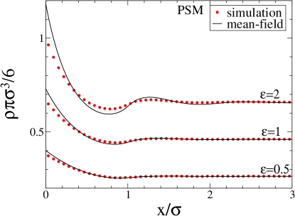
Figure 13: Density profiles of uncharged penetrable spheres near a planar wall. Particle centers are confined in the $x$-axis, $x\in[0,12.5\sigma]$. The number of particles is fixed, $\int dx\,\rho(x)=N=1000$. For Monte Carlo simulation the dimensions of the simulation box are $12.5\times 12.5\times 12.5\sigma$. The box encloses $N=1000$ particles. In the $y$ and $z$ directions periodic boundary conditions are used. The influence of the second wall is minor, and we refer to this system as the wall model.

The mean-field becomes less accurate as $\varepsilon$ increases where it overestimates the contact values, $\rho_{w}$, which are related to the bulk pressure via the contact value theorem,

$$\rho_{w}=\beta P.$$ (128)

Overestimated contact density values imply that the mean-field pressure is larger than the true one, $P_{\rm mf}>P$. To obtain the mean-field pressure we use the virial equation Hansen86 ,

$$\beta P=\rho_{b}-\frac{2\pi}{3}\rho_{b}^{2}\int_{0}^{\infty}dr\,r^{3}g(r)\frac{\partial\beta u(r)}{\partial r},$$ (129)

from which we discard correlations, $g(r)=1$, according to the mean-field procedure, and we get

$$\beta P_{\rm mf}=\rho_{b}+\frac{\varepsilon\rho_{b}^{2}}{2}\Big{(}\frac{4\pi\sigma^{3}}{3}\Big{)},$$ (130)

where we used $\frac{\partial\beta u(r)}{\partial r}=-\varepsilon\delta(r-\sigma)$. The mean-field contact value theorem for penetrable spheres, therefore, is

$$\rho_{w}=\rho_{b}+\frac{\varepsilon\rho_{b}^{2}}{2}\Big{(}\frac{4\pi\sigma^{3}}{3}\Big{)}.$$ (131)

The lower contact density for a true system implies a neglect of correlations in the mean-field approximation.

Having in mind hard-spheres as a model system for excluded volume interactions, we can make contact with it by setting $\varepsilon=1$, where the resulting mean-field pressure,

$$\beta P_{\rm mf}=\rho_{b}(1+4\eta),$$ (132)

agrees to the second virial term with the the pressure for hard-spheres, where $\eta=\pi\rho\sigma^{3}/6$ is the packing fraction.

We next consider charged penetrable spheres with $\varepsilon=1$ and solve Eq. (125) and Eq. (126) for symmetric $1:1$ electrolyte. For the wall model the boundary conditions are the same as for the standard PB equation, and the contact value theorem is

$$\rho_{w}=\rho_{b}(1+4\eta)+\frac{\beta\sigma_{c}^{2}}{2\epsilon}.$$ (133)

In Fig. (14) we plot density profiles for counterions near a charged wall. In comparison with the standard PB equation, the penetrable sphere ions generate a non-monotonic structure of a double-layer, where we see the emergence of a secondary peak. The structure is a result of overcrowding, where counterions coming to neutralize the surface charge cannot be packed too closely together.

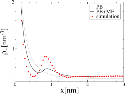
Figure 14: The counterion density near a charged wall. The system is confined between two charged walls at $x=0$ and $x=6\,{\rm nm}$ and the surface charge is $\sigma_{c}=-0.2\,{\rm Cm^{-2}}$. The other parameters are: the Bjerrum length $\lambda_{B}=0.72\,{\rm nm}$, and the diameter of penetrable spheres $\sigma=0.8{\rm nm}$. There is no dialectric discontinuity across an interface. The number of cations is $\int dx\,\rho_{i}(x)=N_{i}=300$ and $N_{+}=N_{-}$. The penetrability parameter is set to $\varepsilon=1$. For simulation we used the hard-sphere limit, $\varepsilon\to\infty$.

The simulation results for hard-sphere particles with the same diameter yield a profile with stronger structure. The penetrable sphere model captures only qualitatively these features.

The present model can be used to study ion specific effects. For neutral surfaces, size asymmetry can lead to different density profiles of ions with the same valance number. This leads to charge build-up across an interface. In Fig. (15) we show density profiles near a neutral wall for a $1:1$ electrolyte with size asymmetry. The larger cations exhibit greater structure and are squeezed against the wall which, in turn, leads to a charge build-up that pulls anions. Simulation results for hard-spheres with the same diameters show similar profiles, however, anions have greater structure as they are depleted from the immediate wall vicinity.

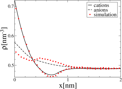
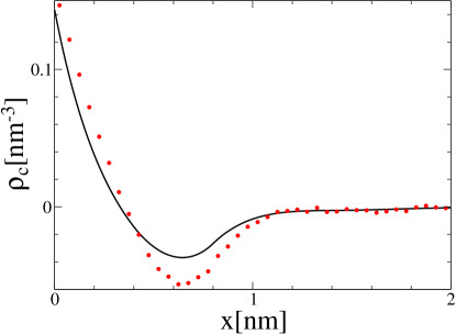
Figure 15: Density profiles of cations, anions, and of total charge near an uncharged wall. Two parallel uncharged plates at $x=0$ and $x=6\,{\rm nm}$ confine all particle centers. The dielectric constant is the same across an interface. The Bjerrum lenght is $\lambda_{B}=0.72\,{\rm nm}$, the ion sizes are $\sigma_{++}=0.8\,{\rm nm}$, $\sigma_{--}=0\,{\rm nm}$, and $\sigma_{+-}=0.4\,{\rm nm}$, and $\int dx\rho_{i}(x)=N_{i}$ where $N_{+}=N_{-}=300$. The simulation was done for the same system but for hard-spheres, $\varepsilon\to\infty$, while in the numerical model we used $\varepsilon=1$.

V.2 short-range interactions beyond the mean-field

In this section we develop a more accurate implementation of short-range interactions, while keeping electrostatics at the mean-field level. Such a procedure introduces asymmetric treatment of different parts of a pair potential. To formally set up and justify this asymmetry of methods, we consider the scaled pair potential,

$$u_{ij}^{\lambda}=u_{ij}^{\rm hs}+\lambda\Bigg{(}\frac{q_{i}q_{j}}{4\pi\epsilon|{\bf r}-{\bf r}^{\prime}|}\Bigg{)},$$ (134)

where $u^{\rm hs}_{ij}$ is the hard-sphere potential, and $\lambda$ is the scaling parameter. For $\lambda=0$ a hard-sphere system is recovered. The density of all ions is independent of $\lambda$ and is kept fixed by the external electrostatic potential, $\psi_{\rm ext}^{\lambda}$. The partition function for this system is

$$Z_{\lambda}=\frac{1}{\prod_{j=1}^{K}(N_{j}!\Lambda^{3N_{j}})}\int\prod_{i=1}^{N}d{\bf r}_{i}e^{-\beta\sum_{i}^{N}Q_{i}\psi_{\rm ext}^{\lambda}({\bf r}_{i})}e^{-\frac{\beta}{2}\sum_{i,j}^{N}\big{[}\lambda\frac{Q_{i}Q_{j}}{4\pi\epsilon|{\bf r}_{i}-{\bf r}_{j}|}+u_{ij}^{\rm hs}({\bf r}_{i},{\bf r}_{j})\big{]}},$$ (135)

where $N=\sum_{j=1}^{K}N_{j}$ is the total number of particles, $N_{j}$ is the number of particles of a species $i$, and the charges $\{Q_{i}\}$ have the following values $Q_{N_{j-1}+1}=Q_{N_{j-1}+2}=\dots=\dots=Q_{N_{j-1}+N_{j}}=q_{j}$, where $q_{i}$ is the charge of a species $i$. The exact functional form of $\psi_{\rm ext}^{\lambda}({\bf r})$ is not needed and it will not appear in the final result. It is sufficient to know that it keeps densities fixed at their physical shape for any value $\lambda$, and $\psi_{\rm ext}^{\lambda=1}$ recovers the true external potential, $\psi_{\rm ext}$.

The free energy, $\beta F=-\log Z$, is obtained from thermodynamic integration,

$$F[\{\rho_{i}\}] = F_{\lambda=0}[\{\rho_{i}\}]+\int_{0}^{1}d\lambda\,\frac{\partial F_{\lambda}}{\partial\lambda}$$

$$= F_{\rm id}[\{\rho_{i}\}]+F^{\rm hs}_{\rm ex}[\{\rho_{i}\}]+\int d{\bf r}\,\rho_{c}({\bf r})\psi_{\rm ext}^{\lambda=0}({\bf r})+\int_{0}^{1}d\lambda\,\frac{\partial F_{\lambda}}{\partial\lambda},$$

where $F_{\rm ex}^{\rm hs}[\rho]$ is the excess free energy due to hard-sphere interactions and is a functional of density only. The integrand of the last term after evaluation is

$$\frac{\partial F_{\lambda}}{\partial\lambda}=\int d{\bf r}\,\rho_{c}({\bf r})\frac{\partial\psi_{\rm ext}^{\lambda}({\bf r})}{\partial\lambda}+\frac{1}{2}\sum_{i,j}^{K}\int d{\bf r}\int d{\bf r}^{\prime}\,\frac{q_{i}\rho_{i}({\bf r})q_{j}\rho_{j}({\bf r}^{\prime})}{4\pi\epsilon|{\bf r}-{\bf r}^{\prime}|}g^{\lambda}_{ij}({\bf r},{\bf r}^{\prime}),$$ (137)

where $g_{ij}=1+h_{ij}$. Inserting this into Eq. (LABEL:eq:F_lambda) we get

$$F[\{\rho_{i}\}] = F_{\rm id}[\{\rho_{i}\}]+F^{\rm hs}_{\rm ex}[\{\rho_{i}\}]+\int\!\!d{\bf r}\,\rho_{c}({\bf r})\psi_{\rm ext}({\bf r})+\frac{1}{2}\int\!\!d{\bf r}\!\!\int\!\!d{\bf r}^{\prime}\,\frac{\rho_{c}({\bf r})\rho_{c}({\bf r}^{\prime})}{4\pi\epsilon|{\bf r}-{\bf r}^{\prime}|}$$

$$+ \frac{1}{2}\sum_{i,j}^{K}\int\!\!d{\bf r}\!\!\int\!\!d{\bf r}^{\prime}\,\frac{q_{i}\rho_{i}({\bf r})q_{j}\rho_{j}({\bf r}^{\prime})}{4\pi\epsilon|{\bf r}-{\bf r}^{\prime}|}\int_{0}^{1}d\lambda\,h_{ij}^{\lambda}({\bf r},{\bf r}^{\prime}).$$

By setting correlations to zero, $h_{ij}^{\lambda}=0$,

$$F[\{\rho_{i}\}]\approx F_{\rm id}[\{\rho_{i}\}]+F^{\rm hs}_{\rm ex}[\{\rho_{i}\}]+\int d{\bf r}\,\rho_{c}({\bf r})\psi_{\rm ext}({\bf r})+\frac{1}{2}\int d{\bf r}\int d{\bf r}^{\prime}\,\frac{\rho_{c}({\bf r})\rho_{c}({\bf r}^{\prime})}{4\pi\epsilon|{\bf r}-{\bf r}^{\prime}|},$$ (139)

we have an approximation that completely neglects terms coupling the electrostatic and hard-core interactions, and that consists of the free energy for hard-spheres plus the mean-field electrostatic correction.

Densities are obtained from the minimum condition, $\frac{\delta F}{\delta\rho_{i}({\bf r})}=0$, and

$$\rho_{i}({\bf r})=c_{i}\exp\Big{[}-\beta q_{i}\psi({\bf r})-\frac{\delta\beta F^{\rm hs}_{\rm ex}}{\delta\rho_{i}({\bf r})}+\beta\mu_{\rm ex}\Big{]},$$ (140)

where $\mu_{\rm ex}=\frac{\partial F_{\rm ex}^{\rm hs}}{\partial\rho}|_{\rho=\rho_{b}}$ is the excess chemical potential over the ideal contribution, $\mu_{\rm id}=\log\rho_{b}\Lambda^{3}$, and $\psi$ is the total electrostatic potential. Implementing this into the Poisson equation we get

$$-\epsilon\nabla^{2}\psi=\sum_{i=1}^{K}c_{i}q_{i}\exp\Big{[}-\beta ez_{i}\psi-\frac{\delta\beta F^{\rm hs}_{\rm ex}}{\delta\rho_{i}({\bf r})}+\beta\mu_{\rm ex}\Big{]}.$$ (141)

Then for $1:1$ electrolyte with all ions having the same size,

$$\epsilon\nabla^{2}\psi=2c_{s}e\sinh(\beta e\psi)\exp\Big{[}-\frac{\beta\delta F_{\rm ex}^{\rm hs}}{\delta\rho}+\beta\mu_{\rm ex}\Big{]}$$ (142)

where $\rho=\rho_{+}+\rho_{-}$ is

$$\rho=2c_{s}\cosh(\beta e\psi)\exp\Big{[}-\frac{\beta\delta F_{\rm ex}^{\rm hs}}{\delta\rho}+\beta\mu_{\rm ex}\Big{]}.$$ (143)

V.2.1 perturbative expansion and the dilute limit

To complete the approximation it remains to find an expression for the excess free energy. The first two terms of the virial expansion for $F^{\rm hs}_{\rm ex}$ are Evans79

$$F_{\rm ex} = \frac{1}{2}\int\!\!d{\bf r}_{1}\!\!\int\!\!d{\bf r}_{2}\,\rho({\bf r}_{1})\rho({\bf r}_{2})\bar{f}(r_{12})$$ (144)

$$+ \frac{1}{6}\int\!\!d{\bf r}_{1}\!\!\int\!\!d{\bf r}_{2}\!\!\int\!\!d{\bf r}_{3}\,\rho({\bf r}_{1})\rho({\bf r}_{2})\rho({\bf r}_{3})\bar{f}(r_{12})\bar{f}(r_{23})\bar{f}(r_{31})$$

$$+ \dots$$

where $\bar{f}(r)=1-e^{-\beta u(r)}$ is the negative Mayer $f$-function, and for hard-spheres is given by the Heaviside function, $\bar{f}(r)=\theta(\sigma-r)$. In the dilute limit the first term dominates and constitutes an accurate approximation,

$$\lim_{\rho\to 0}F^{\rm hs}_{\rm ex}=\frac{1}{2}\int d{\bf r}\int d{\bf r}^{\prime}\,\rho({\bf r}^{\prime})\rho({\bf r}^{\prime})\theta(\sigma-|{\bf r}-{\bf r}^{\prime}|),$$ (145)

which yields

$$\frac{\delta F^{\rm hs}_{\rm ex}}{\delta\rho({\bf r})}=\int d{\bf r}^{\prime}\,\rho({\bf r}^{\prime})\theta(\sigma-|{\bf r}-{\bf r}^{\prime}|),$$ (146)

and the number density becomes

$$\rho_{\pm}({\bf r})=c_{b}e^{\mp\beta e\psi({\bf r})-\int d{\bf r}^{\prime}\,(\rho({\bf r}^{\prime})-2c_{b})\theta(\sigma-|{\bf r}-{\bf r}^{\prime}|)}.$$ (147)

Incidentally, the dilute limit approximation is the same as the mean-field implementation of the penetrable sphere interactions with $\varepsilon=1$, as both approximations are designed to give the lowest order term of the virial expansion for $F_{\rm ex}$ (see Fig. (14) and Fig. (15) for performance of the dilute limit approximation).

V.2.2 nonperturbative approach

Further expansion of the excess free energy does not constitute an efficient scheme. Already the second lowest term involves the three-body overlap contributions that numerically is difficult to deal with. A more powerful approach is a nonperturbative scheme. A nonperturbative construction keeps numerical complexity of the dilute limit approximation but incorporates additional terms (generally an infinite set of terms) that lead to accurate behavior for some limiting condition.

One example is the weighted density approximation of Ref.Tarazona84 ; Tarazona84b . This approximation is constructed in terms of weighted density which constitutes a building block of the theory and is suggested from the lowest order term of the virial series for $F_{\rm ex}^{\rm hs}$,

$$\bar{\rho}({\bf r})=\frac{1}{8}\int d{\bf r}^{\prime}\,\rho({\bf r}^{\prime})\theta(\sigma-|{\bf r}-{\bf r}^{\prime}|).$$ (148)

$\bar{\rho}$ is dimensionless and normalized to recover the packing fraction in a bulk, $\bar{\rho}_{b}=\eta=\pi\sigma^{3}\rho_{b}/6$. The approximation assumes that $F^{\rm hs}_{\rm ex}$ has a general form

$$F_{\rm ex}^{\rm hs}=\int d{\bf r}\,\rho({\bf r})\phi_{\rm ex}(\bar{\rho}({\bf r})),$$ (149)

where $\phi_{\rm ex}$ denotes an excess free energy per particle and is a function of $\bar{\rho}({\bf r})$. Tarazona suggested a generalized Carnahan-Starling approach, where for $\phi_{\rm ex}$ he used the quasi-exact Carnahan-Starling equation Tarazona84 ,

$$\phi_{\rm ex}^{\rm cs}(\bar{\rho}({\bf r}))=\frac{\bar{\rho}({\bf r})(4-3\bar{\rho}({\bf r}))}{(1-\bar{\rho}({\bf r}))^{2}},$$ (150)

but defined as a function of a weighted density. Now, in addition to recovering the dilute limit exactly, the approximation recovers the homogenous limit. Furthermore, the construction satisfies the contact value theorem, $\rho_{w}=P_{\rm cs}$, where $P_{\rm cs}$ is the Carnahan-Starling expression for hard-sphere pressure. The excess chemical potential of this generalized Carnahan-Starling approach is

$$\frac{\delta F^{\rm hs}_{\rm ex}}{\delta\rho({\bf r})}=f_{\rm ex}^{\rm cs}({\bar{\rho}({\bf r})})+\frac{1}{8}\int d{\bf r}^{\prime}\,\rho({\bf r}^{\prime})\frac{\partial f_{\rm ex}^{\rm cs}}{\partial\bar{\rho}({\bf r}^{\prime})}\theta(\sigma-|{\bf r}-{\bf r}^{\prime}|),$$ (151)

and the densities of ionic species are obtained from Eq. (140).

A nonperturbative construction can be further improved by increasing the number of weighted densities as building blocks of the theory. Some improvements where implemented as a result of careful studies of the direct correlation function, which suggested a density dependent weight function Evans92 . The breakthrough approach, however, came with the Rosenfeld’s fundamental measure theory Rosenfeld89 . Motivated (at least in part) by desire to construct a theory that recovers the 1D limit behavior (a property later referred to as the dimensional crossover), Rosenfeld obtained a new set of weight functions by decomposing the Heaviside step function,

$$\theta(\sigma_{ij}-|{\bf r}_{i}-{\bf r}_{j}|) = \omega_{3}^{i}\!\otimes\!\omega_{0}^{j}+\omega_{0}^{i}\!\otimes\!\omega_{3}^{j}+\omega_{2}^{i}\!\otimes\!\omega_{1}^{j}+\omega_{1}^{i}\!\otimes\!\omega_{2}^{j}$$ (152)

$$- {\boldsymbol{\omega}}_{2}^{i}\!\otimes\!{\boldsymbol{\omega}}_{1}^{j}-{\boldsymbol{\omega}}_{2}^{i}\!\otimes\!{\boldsymbol{\omega}}_{1}^{j},$$

where

$$\omega_{\alpha}\otimes\omega_{\beta}=\int d{\bf r}^{\prime}\,\omega_{\alpha}^{i}({\bf r}^{\prime}-{\bf r}_{i})\omega_{\beta}^{j}({\bf r}^{\prime}-{\bf r}_{j}),$$ (153)

and the relevant weight functions are

$$\omega_{3}^{i}({\bf r})=\theta(R_{i}-r),$$

$$\omega_{2}^{i}({\bf r})=\delta(R_{i}-r),$$

$${\boldsymbol{\omega}}_{2}^{i}({\bf r})=\frac{\bf r}{r}\delta(R_{i}-r),$$

and $\omega_{1}^{i}({\bf r})=\omega_{2}^{i}({\bf r})/(4\pi R_{i})$, $\omega_{0}^{i}({\bf r})=\omega_{2}^{i}({\bf r})/(4\pi R_{i}^{2})$, and ${\boldsymbol{\omega}}_{1}^{i}({\bf r})={\boldsymbol{\omega}}_{2}^{i}({\bf r})/(4\pi R_{i})$. The six weighted densities that result are,

$$n_{\alpha}=\sum_{i=1}^{K}\int d{\bf r}^{\prime}\,\rho_{i}({\bf r}^{\prime})\omega^{i}_{\alpha}({\bf r}-{\bf r}^{\prime}),$$ (154)

and a general formula for the excess free energy is

$$\beta F_{\rm ex}^{\rm hs}=\int d{\bf r}\,\Phi^{\rm RF}(\{n_{\alpha}({\bf r})\}).$$ (155)

Based on the scaled particle theory results Lebowitz59 ; Corti04 ; Stillinger06 , Rosenfeld came up with the following functional form Rosenfeld89 ; Tarazona08 ; Evans09 ; Roth10 ,

$$\Phi^{\rm RF} = -n_{0}\log(1-n_{3})+\frac{n_{1}n_{2}-{\bf n}_{1}\cdot{\bf n}_{2}}{1-n_{3}}+\frac{n_{2}^{3}-3n_{2}({\bf n}_{2}\cdot{\bf n}_{2})}{24\pi(1-n_{3})^{2}}.$$

The construction also recovers the PY direct correlation function for homogenous liquids.

In Fig. (16) we plot the counterion density profiles for a symmetrical electrolyte $1:1$ confined between two parallel hard walls. The conditions are the same as in Fig. (14). The WDA gives improvements over the dilute limit approximation, but the DFT fundamental measure theory results agree most closely with the simulation.

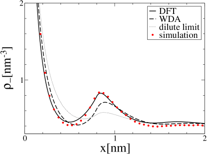
Figure 16: The counterion density near a charged wall for the DFT scheme. Conditions as in Fig. (14). DFT denotes the density functional theory based on the fundamental measure theory Rosenfeld89 , and WDA denotes the weighted density approximation based on the generalized Carnahan-Starling equation Tarazona84 .

In Fig. (17) we plot density profiles for a $1:1$ electrolyte with size asymmetry confined by uncharged walls. The conditions are the same as in Fig. (15). The DFT here is less accurate, although the charge density profile quite well agrees with simulation. The disparity can be traced to the lack of correlations in the mean-field treatment of electrostatics, which become important for an uncharged wall system. The presence of correlations is best seen in the contact density, related to the pressure via the contact value theorem, which is lower in the simulation results, and which indicates negative correlational contributions due to formation of Bjerrum pairs Yan93 .

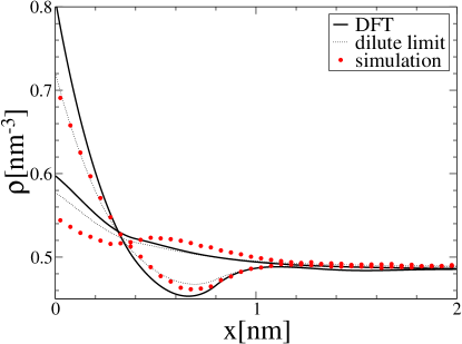
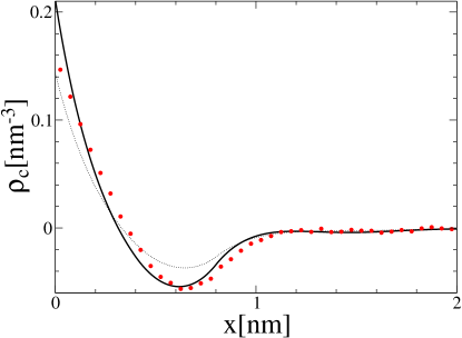
Figure 17: Density profiles near an uncharged wall for various approximations. Conditions as in Fig. (15).

V.2.3 Correlations

The results in Fig. (17) for neutral confinement indicate that despite of highly accurate expression for hard-core interactions, $F_{\rm ex}^{\rm hs}$, the mean-field treatment of electrostatics is not sufficient and the correlations play a dominant role. The neglected correlational contribution to the free energy, taken out of the complete expression in Eq. (LABEL:eq:F_lambda2), is

$$F_{\rm c}=\frac{1}{2}\sum_{i,j}^{K}\int\!\!d{\bf r}\!\!\int\!\!d{\bf r}^{\prime}\,\frac{q_{i}\rho_{i}({\bf r})q_{j}\rho_{j}({\bf r}^{\prime})}{4\pi\epsilon|{\bf r}-{\bf r}^{\prime}|}\int_{0}^{1}d\lambda\,h_{ij}^{\lambda}({\bf r},{\bf r}^{\prime}).$$ (157)

As $\lambda\to 0$, $h^{\lambda}_{ij}$ does not vanish, but instead $h^{\lambda}_{ij}\to h^{\rm hs}_{ij}$.

Applied to homogenous electrolytes, the formula in Eq. (157) yields the charging process formula,

$$f_{\rm c} = \frac{1}{2}\sum_{i=1}^{K}q_{i}c_{i}\int_{0}^{1}d\lambda\,\Bigg{[}4\pi\int_{0}^{\infty}dr\,r^{2}\sum_{j=1}^{K}\frac{q_{j}c_{j}h^{\lambda}_{ij}(r)}{4\pi\epsilon r}\Bigg{]},$$ (158)

where $f_{c}=F_{c}/V$. By identifying the term

$$\rho_{c,i}^{\lambda}(r)=\sum_{j=1}^{K}q_{j}c_{j}h^{\lambda}_{ij}(r)$$ (159)

as the charge distribution around an ion of the species $i$ fixed at the origin (constituting the charge correlation hole), the term in brackets becomes an electrostatic potential that a test ion of the species $i$ feels due to surrounding ions in the system,

$$f_{\rm c}=\frac{1}{2}\sum_{i=1}^{K}q_{i}c_{i}\int_{0}^{1}d\lambda\,\psi_{i}^{\lambda},$$ (160)

where the superscript $\lambda$ indicates that the interactions are scaled. The formula is the expression of the ”charging process”, a common route for obtaining the correlational free energy. Substituting for $\psi^{\lambda}$ the linear Debye-Hückel solution leads to the Debye charging process, which for $1:1$ electrolyte of ions of the same size becomes Yan02 ,

$$q_{i}\psi_{i}^{\lambda}=-\frac{e}{4\pi\epsilon}\Bigg{[}\frac{\kappa\sqrt{\lambda}}{1+\kappa\sigma\sqrt{\lambda}}\Bigg{]},$$ (161)

and

$$\beta f_{c} = -\frac{1}{4\pi\sigma^{3}}\Bigg{[}\log(\kappa\sigma+1)-\kappa\sigma+\frac{(\kappa\sigma)^{2}}{2}\Bigg{]}.$$ (162)

This correlation term constitutes a weak-coupling correction and it does not capture the formation of Bjerrum pairs Yan93 . It gives, however, some estimate of what the contributions of neglected correlations are.

Application of the charging process to inhomogeneous electrolytes is not easy as it requires the precise functional form for $\psi_{\rm ext}^{\lambda}({\bf r})$ which ensures that densities remain constant throughout charging. The implementation of coupled contributions of hard-core and electrostatic contributions remains a challenge. There are some perturbative extensions to the DFT theory based on the reference fluid density Rosenfeld93 ; Eisenberg03 and which address this issue.

V.3 local schemes

After reviewing nonlocal approximations for hard-sphere interactions, it may seem a regression to discuss next local approximations. Nonlocal construction based on weighted densities captures discrete structure of a fluid and is found to satisfy the contact value theorem sum rule. A local construction, on the other hand, is expressed in terms of local density (or a weighted density with a delta weight function), and as such, it does not posses discrete structure of a liquid that is implicit in weight functions, and fails to satisfy the contact value theorem Frydel12 . In other words, density profiles produced by the local type of an approximation are unphysical.

Then why even bother with local approximations? The first answer is simplicity. But this does not justify a model as a description of the world. A more reasonable justification may sound like this. For true electrolytes as they are found in laboratories the exact nature of the excluded volume interactions is not known with precision and there are many different and complex contributions. The hard-sphere model is itself an idealization. The local approximation, in spite of its shortcomings, can offer a first glance and an estimate of excluded volume effects. One, however, has to know how to interpret such a local approximation. The structureless density profile cannot be read as physical. The saturation effect of a local density triggered by overcrowding is an artifact of the model. But although density is unphysical, it does not mean that every other quantity that follows is equally so. For example, the incorrect contact density does not imply an incorrect contact potential. In fact, the contact potential values were found to be reasonably well estimated by a local scheme Frydel12 . The local saturation of a density profile, its flattening near a charged surface, captures qualitatively the fact that a double-layer is elongated due to excluded volume effects, and this in turn reproduces, at least qualitatively, the increase in electrostatic potential that is less efficiently screened.

Within local approximation the excess free energy is

$$F_{\rm ex}^{\rm hs}=\int d{\bf r}\,f_{\rm ex}(\rho({\bf r})),$$ (163)

where the excess free energy density $f_{\rm ex}$ is a function of a local density, and a functional derivative becomes classical derivative,

$$\frac{\delta F_{\rm ex}^{\rm hs}}{\delta\rho({\bf r})}=\frac{\partial f_{\rm ex}}{\partial\rho({\bf r})}=\mu_{\rm ex}(\rho({\bf r})),$$ (164)

which yields the following density

$$\rho_{i}({\bf r})=c_{i}e^{-\beta\big{[}q_{i}\psi({\bf r})+\mu_{\rm ex}(\rho({\bf r}))-\mu_{\rm ex}(\rho_{b})\big{]}},$$ (165)

The mean-field Poisson equation becomes,

$$\epsilon\nabla^{2}\psi({\bf r})=-\sum_{i=1}^{K}q_{i}c_{i}e^{-\beta\big{[}q_{i}\psi({\bf r})+\mu_{\rm ex}(\rho({\bf r}))-\mu_{\rm ex}(\rho_{b})\big{]}}.$$ (166)

We assume that all diameters are the same.

To complete the model, it remains to choose expression for $\mu_{\rm ex}$. There are several equations of state we can choose from. The hard-sphere model (or the quasi-exact Carnahan-Starling equation) is

$$\frac{\beta P}{\rho}=\frac{1+\eta+\eta^{2}-\eta^{3}}{(1-\eta)^{3}}~{}~{}~{}\longrightarrow~{}~{}~{}\beta\mu_{\rm ex}=\frac{8\eta-9\eta^{2}+3\eta^{3}}{(1-\eta)^{3}}.$$ (167)

A cruder van der Waals model for excluded volume interactions is

$$\frac{\beta P}{\rho}=\frac{1}{1-\nu\rho}~{}~{}~{}\longrightarrow~{}~{}~{}\beta\mu_{\rm ex}=-\log(1-\nu\rho)+\frac{\nu\rho}{1-\nu\rho},$$ (168)

where $\nu$ denotes the excluded volume. Finally, the lattice-gas model is David97

$$\frac{\beta P}{\rho}=-\frac{\log(1-\eta)}{\eta}~{}~{}~{}\longrightarrow~{}~{}~{}\beta\mu_{\rm ex}=-\log(1-\eta).$$ (169)

In Fig. (18) we compare the lattice-gas equation of state with that for hard-spheres. The two models are completely different. There is no agreement in any limit. The lattice-gas curve is relatively flat and then exhibits a sharp rise as $\eta\to 1$.

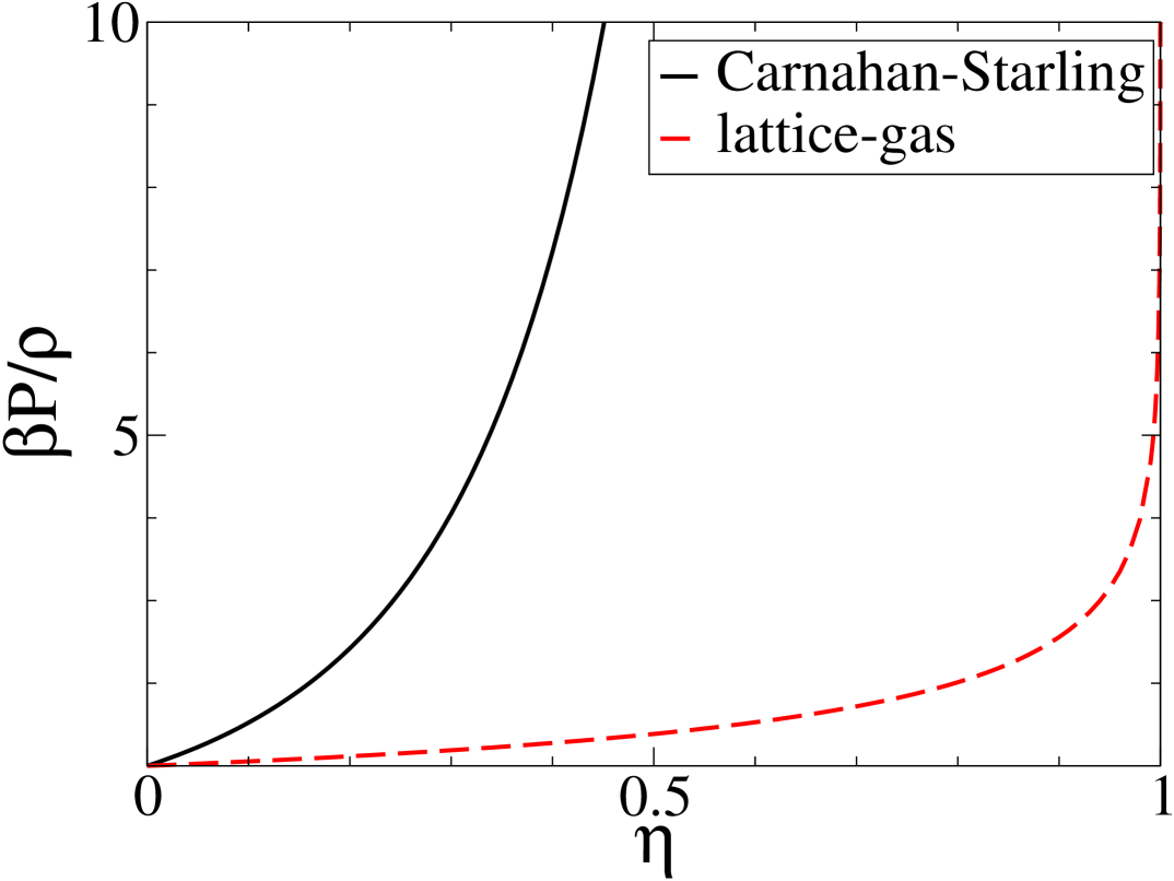
Figure 18: The equation of state $\beta P/\rho$ as a function of a packing fraction $\eta=\pi\sigma^{3}/6$.

The lattice-gas model has advantage in its simple analytical form. The probability for successful insertion of a particle into a hard-sphere fluid is $e^{-\beta\mu_{\rm ex}}=1-\eta$. The result is intuitive and expresses the fraction of an available volume not taken up by other particles. This simple result leads to the following density

$$\rho_{i}=c_{i}e^{-\beta q_{i}\psi}\bigg{(}\frac{1-\nu\sum_{i=1}^{K}\rho_{i}}{1-\nu\sum_{i=1}^{K}c_{i}}\bigg{)},$$ (170)

where $\nu=\pi\sigma^{3}/6$ is the sphere volume. After some algebraic manipulation we get

$$\rho_{i}=\frac{c_{i}e^{-\beta q_{i}\psi}}{1+\nu\sum_{i=1}^{K}c_{i}(e^{-\beta q_{i}\psi}-1)}.$$ (171)

In the limit $\psi\to 0$, the standard Poisson-Boltzmann equation is recovered, $\rho_{i}\to c_{i}e^{-\beta q_{i}\psi}$. But if potential becomes large a density cannot increase indefinitely as it is bounded from above, $\rho\leq\nu^{-1}$. The modified Poisson-Boltzmann equation that results is

$$\epsilon\nabla^{2}\psi=-\frac{\sum_{i=1}^{K}q_{i}c_{i}e^{-\beta q_{i}\psi}}{1+\nu\sum_{i=1}^{K}c_{i}(e^{-\beta q_{i}\psi}-1)}.$$ (172)

Specializing to the $1:1$ electrolyte we get David97

$$\epsilon\nabla^{2}\psi=-\frac{2ec_{s}\sinh\beta e\psi}{1+2\nu c_{s}(\cosh\beta e\psi-1)}$$ (173)

This is the modified Poisson-Boltzmann equation as derived in David97 . It yields the same boundary condition as the standard PB equation. Also, the model does not lead to the true contact value theorem, $\rho_{w}=P+\frac{\beta\sigma_{c}^{2}}{2\epsilon}$, where in place of $P$ we use the lattice-gas pressure in Eq. (169). Instead, it obeys another contact value relation,

$$\rho_{w}=\frac{1}{\nu}\bigg{[}1-(1-\eta_{b})e^{-\beta\sigma_{c}^{2}\nu/2\epsilon}\bigg{]},$$ (174)

since, as was said before, the density is not physical. The model introduces a new length scale, $\nu\sigma_{c}$, that corresponds to the width of counterion layer that would form if all counterions were allowed to come to a charged surface and the exceeded volume effect was the only interaction. Now, even for the vanishing screening length, $\kappa^{-1}\to 0$, a double-layer will have thickness $\nu\sigma_{c}$ (where $\kappa=\sqrt{8\pi c_{s}\lambda_{B}}$ is the Debye screening parameter). Based on these two competing length scales it is possible to estimate the importance of the excluded volume effects. If $\nu\sigma_{c}>\kappa^{-1}$, we should expect the excluded volume effects to play a significant role.

In Fig. (19) we compare the results of the modified PB equation with other approximations. The density profile of the modified PB equation shows unphysical saturation of a local density. The standard PB equation, in fact, yields better agreement with the DFT near a wall including a contact density. The modified PB equation, however, yields better results for electrostatic potential which comes close to the DFT approximation at a wall contact.

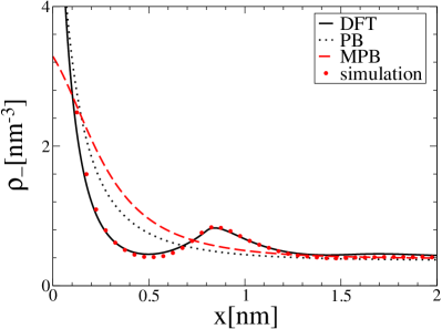
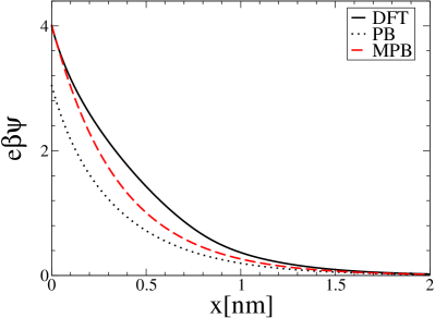
Figure 19: Counterion density and potential profiles for the conditions as in Fig. (14) and Fig. (14).

The modified PB equation captures the fact that the surface charge is less efficient screening when the excluded volume interactions are involved. In Fig. (20) we plot contact potential as a function of the surface charge. The modified PB equation captures the influence of the excluded volume effects in relation to the standard PB equation. As $\sigma_{c}$ becomes large, the agreement with the DFT is less perfect.

Figure 20: Electrostatic potential at a wall contact as a function of a surface charge. The system parameters are : $\lambda_{B}=0.72\,{\rm nm}$, $\sigma=0.8\,{\rm nm}$, $c_{s}=0.3\,{\rm M}$.

The question still remains how using the Carnahan-Starling equation of state for the local approximation would change the results. After all, when choosing the lattice-gas equation of state, the only criterion that was followed was simplicity. It turns out that the equation of state for hard-spheres gives worse agreement with the DFT and it exaggerates overcrowding by yielding too high contact potentials. It somewhat seems a stroke of luck that the lattice-gas equation of state provides both simplicity and relative accuracy, suggesting that some cancellation of errors is being involved.

VI Conclusion

The present review provides a framework for constructing various mean-field models for ions with some sort of structure and provides a number of modified PB equations to which this construction leads. All possibilities, of course, cannot be exhausted, but with a large number of detailed constructions it should not be difficult to build a model that fits a given situation. One possible direction to pursue further is to explore in more detail models for ions with finite charge distribution, all the way until making contact with polyelectrolytes, whose single configuration is represented with a Brownian walk type of a distribution. What was also left out from the review were models that combine several structures together. For example, a spherical charge distribution could be supplemented with repulsive Gaussian interactions representing a self-avoiding walk of two polymer chains. This would render a more realistic representation of polyelectrolytes. But again, such combinations are not difficult to infer from provided constructions. It is, in fact, one of the goals of this review to motivate such new constructions.

The review also leaves some suggestions for the future work. As there is an ever increasing number of new macromolecules with interactions ranging from ultrasoft to hard-core, particles whose shape is not fixed but flexible, there is an ever growing demand for their accurate representation. One possible way to proceed is to explore the present mean-field framework and implement some sort of elastic behavior to allow charge distributions to deform into most optimal shape, so that near an interface particles and their mutual interactions are modified. Similar elastic behavior could be supplemented to non-electrostatic type of interactions.

As far as the treatment of short-range non-electrostatic interactions is concerned, the mean-field is sufficient if interactions are soft. The handling of hard-sphere interactions, however, is far more challenging. The most efficient theory for hard-core interactions, the fundamental measure DFT, shows shortcomings even for the weak-coupling limit conditions. To construct a more accurate theory it is, therefore, necessary to incorporate correlations, thus, to go beyond the conveniences of the mean-field. But for charged hard-core particles correlations are difficult to implement as they couple hard-core and electrostatic interactions. The treatment of these coupled, short- and long-range, interactions is, in fact, one of the most outstanding problems of soft-matter electrostatics.

The idea of a modified PB equation, of representing more physics and more accurately through a model based on a single differential equation, has caught some momentum, and there are models that go beyond the mean-field and attempt to implement effects seen in the intermediate- and strong-coupling limit. An exemplary case is the work by Bazant et al. Bazant11 ; Bazant12 where the authors suggested the modified PB equation with dielectric constant represented as a linear differential operator. The model aims to represent ionic liquids were opposite ions strongly associate and coexist as a Bjerrum pair rather than as free ions.

There is an additional motivation for pursuing various mean-field constructions. Simple models such as charged hard-spheres are easy to simulate, and for these systems one could simply stick to simulations to cover the entire range of electrostatics, from weak- to strong-coupling regime. But there are systems that are not easy to simulate. This is especially true for polarizable ions and for explicit treatment of water. For these cases the mean-field construction provides a real alternative, sometimes the only choice.

Finally, it should be reminded and stressed one more time what the boundaries of the mean-field treatment are and what type of electrostatics it is capable of representing. Not only it neglects correlational corrections already active in the weak-coupling regime, but it completely fails in the strong-coupling limit as a predictive tool. The strong-coupling limit electrostatics calls for different treatments.

99

References

- (1) D. Ben-Yaakov, D. Andelman and D. Harries, J. Phys. Chem. B 113, 6001 (2009).
- (2) F. Hofmeister, Arch. Exp. Pathol. Pharmacol. 24, 247 (1888).
- (3) Y. Zhang, P. S. Cremer, Curr. Opin. Chem. Biol. 10, 658 (2006).
- (4) A. P. dos Santos, A. Diehl and Y. Levin, Langmuir 26, 10778 (2010).
- (5) J. B. Hasted, D. M. Ritson, and C. H. Collie, J. Chem. Phys. 16, 1 (1948).
- (6) D. Ben-Yaakov, D. Andelman and R. Podgornik, J. Chem. Phys. 134, 074705 (2011).
- (7) A. Abrashkin, D. Andelman, and H. Orland, Phys. Rev. Lett. 99, 077801 (2007).
- (8) Y. W. Kim, Y. Yi, and P. A. Pincus, Phys. Rev. Lett. 101, 208305 (2008).
- (9) R.R. Netz, H. Orland, Eur. Phys. J. E 1, 203 (2000).
- (10) W. Klein and H. L. Frisch, J. Chem. Phys. 84, 968 (1986).
- (11) N. Grewe and W. Klein, J. Math. Phys. 18, 1735 (1977).
- (12) A. A. Louis, P. G. Bolhuis, and J. P. Hansen, Phys. Rev. E 62, 7961 (2000).
- (13) A. Naji, M. Kanduč, R. R. Netz, R. Podgornik, ”Exotic electrostatics: unusual features of electrostic interactions between macroions”, in Understanding Soft Condensed Matter via Modeling and Computation (Series in soft condensed matter) Vol. 3, 2010, pp. 265-295.
- (14) P. Linse and V. Lobaskin, Phys. Rev. Lett. 83, 4208 (1999).
- (15) V. I. Perel and B. I. Shklovskii, Physica A 274, 446 (1999).
- (16) B. I. Shklovskii, Phys. Rev. E 60, 5802 (1999).
- (17) A. G. Moreira and R. R. Netz, Europhys. Lett. 52, 705 (2000).
- (18) L. Šamaj and E. Trizac, Phys. Rev. Lett. 106, 078301 (2011).
- (19) I. Rouzina and V. A. Bloomfield, J. Phys. Chem. 100, 9977 (1996).
- (20) Y. Levin, Rep. Prog. Phys. 65, 1577 (2002).
- (21) A. Yu. Grosberg, T. T. Nguyen, and B. I. Shklovskii, Rev. Mod. Phys. 74, 329 (2002)
- (22) A. Levy, D. Andelman, H. Orland, J. Chem. Phys. 139, 164909 (2013).
- (23) J. J Bikerman, Philos. Mag. 33 384 (1942).
- (24) I. Borukhov, D. Andelman, and H. Orland, Phys. Rev. Lett. 79, 435 (1997).
- (25) C. Azuara, H. Orland, M. Bon, P. Koehl, and M. Delarue Biophysical Journal 95, 5587 (2008).
- (26) D. H. Mengistu, K. Bohinc, and S. May, Europhys. Lett. 88 14003 (2009).
- (27) P. Koehl, H. Orland, and M. Delarue, Phys. Rev. Lett. 102, 087801 (2009).
- (28) A. Iglič, E. Gongadze, and K. Bohinc Bioelectrochemistry, 79 223 (2010).
- (29) D. Frydel and M. Oettel, Phys Chem Chem Phys. 13, 4109 (2011).
- (30) D. Frydel and M. Oettel, ”Extended Poisson-Boltzmann descriptions of the electrostatic double layer: implications for charged particles at interfaces”, in ”New challenges in Electrostatics of Soft and Disordered Matter”, Eds. J. Dobnikar, A. Naji, D.Dean and R. Podgornik, Singapore (2014).
- (31) A. Levy, D. Andelman, H. Orland, Phys. Rev. Lett. 108, 227801 (2012).
- (32) F. London, Trans. Farad. Soc. 33, 8 (1937).
- (33) R. R. Netz, J. Phys.: Condens. Matter 16, S2353 (2004).
- (34) R. R. Netz, Curr. Opin. Colloid Interface Sci. 9, 192 (2004).
- (35) L. B. Bhuiyan and C. W. Outhwaite, J. Phys. Chem. 93 1526 (1989).
- (36) D. Frydel, J. Chem. Phys. 134, 234704 (2011).
- (37) M. M. Hatlo, R. van Roij and L. Lue, EPL 97 28010 (2012).
- (38) V. Démery, D. S. Dean and R. Podgornik, J. Chem. Phys. 137, 174903 (2012).
- (39) M. Ma and Z. Xu, http://arxiv.org/pdf/1410.4661
- (40) K. Bohinc, A. Iglič and S. May, Europhys. Lett. 68, 494 (2004).
- (41) S. May, A. Iglic, J. Rescic, S. Maset and K. Bohinc, J. Phys. Chem. B 112, 1685 (2008).
- (42) K. Bohinc, J. Rescic, J. Maset and S. May, J. Chem. Phys. 134, 07411 (2011).
- (43) K. Bohinc, J. M. A. Grime, L. Lue, Soft Matter 8, 5679 (2012).
- (44) C. N. Likos, Phys. Rep. 348, 267 (2001).
- (45) A. A. Louis, P. G. Bolhuis, J.-P. Hansen, and E. J. Meijer, Phys. Rev. Lett. 85, 2522 (2000).
- (46) C. N. Likos, M. Schmidt, and H. Löwen, M. Ballauff and D. Pötschke, Macromolecules 34, 2914 (2001).
- (47) D. Coslovich, J.-P. Hansen and G. Kahl, Soft Matter 7, 1690 (2011).
- (48) D. Coslovich, J.-P. Hansen and G. Kahl, J. Chem. Phys. 134, 244514 (2011).
- (49) A. Nikoubashman, J.-P. Hansen, and G. Kahl, J. Chem. Phys. 137, 094905 (2012).
- (50) P. B. Warren and A. J. Masters, J. Chem. Phys. 138, 074901 (2013).
- (51) M. E. Fisher and Y. Levin, Phys. Rev. Lett. 71, 3826 (1993).
- (52) C. N. Likos, A. Lang, M. Watzlawek, and H. Löwen, Phys. Rev. E 63, 031206 (2001).
- (53) B. M. Mladek, D. Gottwald, G. Kahl, M. Neumann, and C. N. Likos, Phys. Rev. Lett. 96, 045701 (2006).
- (54) C. Marquest and T. A. Witten, J. Phys. France 50, 1267 (1989).
- (55) F. H. Stillinger, J. Chem. Phys. 65, 3968 (1976).
- (56) F. Cinti, T. Macrí, W. Lechner, G. Pupillo and T. Pohl, Nature Communications 5, 3235 (2014).
- (57) D. Frydel, Y. Levin, J. Chem. Phys. 138, 174901 (2013).
- (58) I. Borukhov, Physica A 249, 315 (1998).
- (59) J. Hemmerle, V. Roucoules, G. Fleith, M. Nardin, V. Ball, Ph. Lavalle, P. Marie, J.-C. Voegel, P. Schaaf, Langmuir 21, 10328 (2005).
- (60) D. Mijares, M. Gaitan, B. Polk, D. DeVoe, J. Res. NIST 115, 61 (2010).
- (61) N. Grewe and W. Klein, J. Math. Phys. 18, 1729 (1977).
- (62) W. Klein and N. Grewe, J. Chem. Phys. 72, 5456 (1980).
- (63) W. Kunkin and H. L. Frisch, J. Chem. Phys. 50, 181 (1969).
- (64) T. Naitoh and K. Nagai, J. Stat. Phys. 11, 391 (1974).
- (65) W. Klein, H. Gould, R. A. Ramos, I. Clejan and A. I. Melcuk, Physica A 205, 738 (1994).
- (66) C. N. Likos, M. Watzlawek, and H. Löwen, Phys. Rev. E 58, 3135 (1998).
- (67) M. Schmidt, J. Phys.: Condens. Matter 11, 10163 (1999).
- (68) F. H. Stillinger and D. K. Stillinger, Physica A 244, 358 (1997).
- (69) J. Urbanija, K. Bohinc, A. Bellen, S. Maset, A. Iglič, J. Chem. Phys. 129, 105101 (2008).
- (70) M. Kanduč, A. Naji, R. Podgornik, J. Phys. Condens. Matter. 21, 424103 (2009).
- (71) R. I. Slavchov and T. I. Ivanov, J. Chem. Phys. 140, 074503 (2014).
- (72) F. J. Dyson and A. Lenard, J. Math. Phys. 8, 423 (1967); F. J. Dyson and A. Lenard, J. Math. Phys. 9, 698 (1968); F. J. Dyson, J. Math. Phys. 8, 1538 (1967).
- (73) J. P. Hansen and I.R. McDonald, Theory of Simple Liquids, 2nd ed. (Academic Press, London, 1986).
- (74) R. Evans, Adv. Phys. A 28, 143 (1979).
- (75) P. Tarazona, Mol. Phys. 52, 81 (1984).
- (76) P. Tarazona and R. Evans, Mol. Phys. 52 847 (1984).
- (77) R. Evans, in Fundamentals of Inhomogeneous Fluids, edited by D. Henderson, Chap. 3 (Dekker, New York, 1992), p. 85.
- (78) Y. Rosenfeld, Phys. Rev. Lett. 63, 980 (1989).
- (79) H. Reiss, H. L. Frisch, J. L. Lebowitz, J. Chem. Phys 31, 369 (1959).
- (80) M. Heying and D. S. Corti, J. Phys. Chem. B 108, 19756 (2004).
- (81) F. H. Stillinger, P. G. Debenedetti and S. Chatterjee, J. Chem. Phys. 125, 204504 (2006).
- (82) P. Tarazona, J. A. Cuesta, and Y. Martinez-Raton, Lect. Notes Phys. 753 247 (2008).
- (83) R. Evans, Lecture Notes at 3rd Warsaw School of Statistical Physics (Warsaw University Press, Kazimierz Dolny, 2009) pp. 43- 85.
- (84) R. Roth, J. Phys.: Condens. Matter 22, 063102 (2010).
- (85) Y. Rosenfeld, J. Chem. Phys. 98, 8126 (1993).
- (86) D. Gillespie, W. Nonner, and R. S. Eisenberg, Phys. Rev. E 68, 031503 (2003).
- (87) D. Frydel, Y. Levin, J. Chem. Phys. 137, 164703 (2012).
- (88) M. Z. Bazant, B. D. Storey, and A. A. Kornyshev, Phys. Rev. Lett. 106, 046102 (2011).
- (89) B. D. Storey and M. Z. Bazant, Phys. Rev. E 86, 056303 (2012).
99