A posteriori error estimates
for leap-frog and cosine methods
for second order evolution problems

Abstract

We consider second order explicit and implicit two-step time-discrete schemes for wave-type equations. We derive optimal order a posteriori estimates controlling the time discretization error. Our analysis, has been motivated by the need to provide a posteriori estimates for the popular leap-frog method (also known as Verlet’s method in molecular dynamics literature); it is extended, however, to general cosine-type second order methods. The estimators are based on a novel reconstruction of the time-dependent component of the approximation. Numerical experiments confirm similarity of convergence rates of the proposed estimators and of the theoretical convergence rate of the true error.

1 Introduction

This work is concerned with second order explicit and implicit two-step time-discrete schemes for wave-type equations. Our objective is to derive optimal order a posteriori estimates controlling the time-discretization error. To the best of our knowledge, error control for wave equations, discretized by popular methods is limited so far to first order schemes [9, 13]. Despite the importance of such wave-type problems, the lack of error control for time-discretizations used extensively in applications is probably due to the two-step character of these methods, and the associated technical issues. Our analysis, has been motivated by the need to provide a posteriori estimates for the leap-frog method or, as often termed, Verlet’s method in the molecular dynamics literature. It extends, however to general cosine-type second order methods [5, 6].

Adaptivity and a posteriori error control for parabolic problems have been developed in, e.g., [12, 25, 21, 15, 19, 8, 10, 17]. In particular, as far as time discretization is concerned, all implicit one-step methods can be treated within the framework developed in [2, 20, 3, 4, 18]. Although some of these results apply (directly or after appropriate modifications) to the wave equation also, when written as a first order system and discretised by implicit Runge-Kutta or Galerkin schemes, this framework does not cover popular two-step implicit or explicit time-discretisation methods. The recent results in [9, 13] cover only first order time discrete schemes; see also [1] for certain estimators to standard implicit time-stepping finite element approximations of the wave equation. For earlier works on adaptivity for wave equations from various perspectives we refer, e.g., to [16, 7, 23, 24].

Model problem and notation.

Let $(H,\langle{\cdot},{\cdot}\rangle)$ be a Hilbert space and $\mathcal{A}:[0,T]\to D(\mathcal{A})$, positive definite, self-adjoint, linear operator on $D(\mathcal{A})$, the domain of $\mathcal{A}$, which is assumed to be dense in $H$. For time $t\in(0,T]$, we consider the linear second order hyperbolic problem: find $u:[0,T]\to D(\mathcal{A})$, such that

$$u^{\prime\prime}(t)+\mathcal{A}u(t) =f(t)\quad\text{for }0<t\leq T,$$ (1)

$$u(0) =u_{0},$$

$$u^{\prime}(0) =v_{0},$$

where $f:[0,T]\to H$, $u_{0},v_{0}\in H$.

Leap-frog time-discrete schemes.

We shall be concerned with the popular leap-frog time-discrete scheme for (1). We consider a subdivision of the time interval $(0,T]$ into disjoint subintervals $(t^{n},t^{n+1}]$, $n=0,\dots,N-1$, with $t^{0}=0$ and $t^{N}=T$, and we define $k_{n}:=t^{n+1}-t^{n}$, the time-step. For simplicity of the presentation, we shall assume that $k_{n}=k$ is constant, although this is not a restriction of the analysis below. Despite being two-step, the schemes considered herein can be formulated for variable time steps also, with their consistency and stability properties then being influenced accordingly, cf. [22, 11]; the study of such extensions is out of the scope of this work. We shall use the notation $t^{n+1/2}:=(t^{n+1}+t^{n})/2$.

The time-discrete leap-frog scheme (or Verlet’s method in the terminology of initial value problems or of molecular dynamics) for the wave problem (1) is defined by finding approximations $U^{n+1}\in D(\mathcal{A})$ of the exact values $u^{n+1}:=u(t^{n+1})$, such that:

$$\partial^{2}U^{n+1}+\mathcal{A}U^{n}=f^{n},\quad n=1,\dots,N-1,$$ (2)

where $f^{n}:=f(t^{n})\in H$,

$$\partial^{2}U^{n+1}:=\frac{\partial U^{n+1}-\partial U^{n}}{k}=\frac{U^{n+1}-2U^{n}+U^{n-1}}{k^{2}},$$ (3)

with

$$\partial U^{n+1}:=\frac{U^{n+1}-U^{n}}{k},$$

assuming knowledge of $U^{0}$ and $U^{1}$. We set $U^{0}:=u_{0}$ and we define $U^{1}$ by

$$\frac{\partial U^{1}-v_{0}}{k}+\frac{1}{2}\mathcal{A}U^{0}=\frac{1}{2}f^{0},$$ (4)

where $f^{0}:=f(0)$ and $\partial U^{1}:=(U^{1}-U^{0})/k$. This is a widely used and remarkable method in many ways: it is the only two-step explicit scheme for second order problems which is second order accurate, it has important conservation and geometric properties, as it is symplectic, and it is very natural and simple to formulate and implement. We refer to the review article [14] for a thorough discussion. Explicit schemes, such as (2) are suited for the discretization of wave-type partial differential equations, since their implementation requires a mild CFL-type condition of the form $k/h\leq C$ (in contrast to parabolic problems,) where $h$ stands for the space-discretization parameter.

Cosine methods.

The leap-frog scheme is a member of a general class of two-step methods for second order evolution problems, which are based on the approximation of cosine and are used extensively in practical computations. In a two-step cosine method, for $n=1,\dots,N-1,$ we seek approximations $U^{n+1}$ such that

$$\partial^{2}U^{n+1}+\big{[}\,q_{1}\,\mathcal{A}U^{n+1}-2p_{1}\mathcal{A}U^{n}+q_{1}\,\mathcal{A}U^{n-1}\,\big{]}=\big{[}\,q_{1}\,f^{n+1}-2p_{1}f^{n}+q_{1}\,f^{n-1}\,\big{]},\$$ (5)

where we assume that $p_{1}=q_{1}-\frac{1}{2}$ for second order accuracy; we refer to [5, 6] for a detailed discussion and analysis of general multi-step cosine schemes. In this case, the rational function $r(x)=(1+p_{1}x^{2})/(1+q_{1}x^{2})$ is a second order approximation to the cosine, in the sense that for $|x|$ sufficiently small,

$$|r(x)-\cos(x)|\leq C\,x^{4}\,.$$ (6)

When $q_{1}=0$ the above methods are explicit, and the condition $p_{1}=q_{1}-\frac{1}{2}$ implies that the only explicit second order member of this family is the leap-frog method (2).

In this work, we derive a posteriori error bounds in the $\operatorname{L}^{\infty}($)-in-time-energy-in-space norm of the error. The derived bounds are of optimal order, i.e., of the same order as the error (which is known to be second order) for the class of the schemes considered [5, 6]. This is verified by the numerical experiments presented herein. Our approach is based on the following ingredients: first, we rewrite the schemes as one-step system on staggered time grids. In turn, this can be seen as a second order perturbation of the staggered midpoint method. Further, by introducing appropriate interpolants, we arrive to a form which can be viewed as perturbation of (1) written as a first-order system. Finally, we employ an adaptation of the time reconstruction from [2], yielding the desired a posteriori error estimates. An interesting observation is that our estimates hold without any additional time-step assumption, which at the fully discrete level would correspond to a CFL-type restriction. Thus, in a posteriori analysis, standard stability considerations of time discretisation schemes might influence the behaviour of the estimator, but are not explicitly required; the possible instability is sufficiently reflected by the behaviour of the estimator, see Section 4. Although not done here, by employing space reconstruction techniques it would be possible to derive error estimates for fully discrete schemes in various norms, using ideas from [19, 17, 13].

The remaining of this work is organized as follows. In §2 we reformulate the numerical methods appropriately – this is a crucial step in our approach. We start with the leap-frog method and we continue with providing two alternative reformulations of general cosine methods. In §3 we introduce appropriate time reconstructions and we derive the error bounds. In §4 we present detailed numerical experiments which yield experimental orders of convergence for the estimators that are the same with those of the actual error. Finally, in §5 we draw some concluding remarks.

2 Reformulation of the methods

It will be useful for the analysis to reformulate the methods as a system in two staggered grids.

2.1 Leap-frog

Starting with the leap-frog method, we introduce the auxiliary variable

$$V^{n+1/2}:=\partial U^{n+1},$$ (7)

for $n=0,1,\dots,N-1$, and we set $V^{-1/2}:=2v_{0}-V^{1/2}$. (Note that, then, $v_{0}=(V^{-1/2}+V^{1/2})/2$.) Also, we define $U^{-1}:=U^{0}-kV^{-1/2}$ and we observe that we have

$$v_{0}=\frac{U^{1}-U^{-1}}{2k}.$$

Further, we introduce the notation

$$\partial V^{n+1/2}:=\frac{V^{n+1/2}-V^{n-1/2}}{k},\quad n=0,1,\dots,N-1,$$ (8)

noting that the identity $\partial V^{1/2}=2(\partial U^{1}-v_{0})/k$ also holds.

We can now write the method (2) as a system in the staggered form considered in [14]:

$$\begin{split}&\partial U^{n+1}-V^{n+1/2}=0,\\ \quad&\partial V^{n+1/2}+\mathcal{A}U^{n}=f^{n}\,,\end{split}$$ (9)

for $n=0,1,\dots,N-1$.

Next, our goal is to recast (9) using globally defined piecewise linear functions. We define $U:[-k,T]\to D(\mathcal{A})$ to be the piecewise linear interpolant of the sequence $\{U^{n}\}_{n=-1}^{N}$, at the points $\{t^{n}\}_{n=-1}^{N}$, with $t^{-1}:=-k$. In addition, let $V:[-k/2,t^{N-1/2}]\to D(\mathcal{A})$ be the piecewise linear interpolant of the sequence $\{V^{n+1/2}\}_{n=-1}^{N-1}$, at the points $\{t^{n+1/2}\}_{n=-1}^{N-1}.$ Using the notation

$$\begin{split}U^{n+1/2}:=&\ U(t^{n+1/2}),\\ \quad V^{n}:=&\ V(t^{n}),\qquad n=0,\dots,N-1\,.\end{split}$$ (10)

we, then, have

$$U^{n+1/2}=\frac{1}{2}(U^{n+1}+U^{n}),\quad V^{n}=\frac{1}{2}(V^{n+1/2}+V^{n-1/2}),$$ (11)

for $n=0,1,\dots,N-1$.

Hence, in view of (11), (9) implies

$$\partial U^{n+1}-\frac{1}{2}(V^{n+1}+V^{n}) =-\frac{1}{4}(V^{n+3/2}-2V^{n+1/2}+V^{n-1/2}),$$ (12)

$$\partial V^{n+1/2}+\frac{1}{2}\mathcal{A}(U^{n+1/2}+U^{n-1/2}) =f^{n}+\frac{1}{4}\mathcal{A}(U^{n+1}-2U^{n}+U^{n-1}),$$

for $n=0,\dots,N-1$. Upon defining the piecewise constant residuals

$$R_{U}(t)|_{(t^{n-1/2},t^{n+1/2}]}\equiv R_{U}^{n}:=\frac{1}{4}\mathcal{A}(U^{n+1}-2U^{n}+U^{n-1}),$$

$$R_{V}(t)|_{(t^{n},t^{n+1}]}\equiv R_{V}^{n+1/2}:=-\frac{1}{4}(V^{n+3/2}-2V^{n+1/2}+V^{n-1/2})\,,$$

it is easy to check that, given that the leap-frog method is second order (in both $U^{n}$ and $V^{n+1/2}$), we have $R_{U}^{n}=O(k^{2})$ and $R_{V}^{n+1/2}=O(k^{2}).$ Hence, (12) can be viewed as a second order perturbation of the staggered mid-point method for (1) written as first order system

$$u^{\prime}-v=0\,,$$ (13)

$$v^{\prime}+\mathcal{A}u=f\,.$$

In what follows, it will be useful to rewrite (12) as a perturbation of the continuous system (13). To this end, we introduce two time interpolants onto piecewise linear functions defined on the staggered grids: we define $U_{1}:[0,T]\to D(\mathcal{A})$ to be the piecewise linear interpolant of the sequence $\{U^{n+1/2}\}_{n=-1}^{N-1}$ and $V_{1}:[0,t^{N-1}]\to D(\mathcal{A})$ to be the piecewise linear interpolant of the sequence $\{V^{n}\}_{n=0}^{N-1}$. Then, (12) can be written as

$$U^{\prime}-I_{0}V_{1} =R_{V},$$ (14)

$$V^{\prime}+\mathcal{A}\tilde{I}_{0}U_{1} =\tilde{I}_{0}f+R_{U},$$

where we define the interpolators

$$\begin{split}\tilde{I}_{0}:&\text{ piecewise constant midpoint interpolator on }\{(t^{n-1/2},t^{n+1/2}]\}_{n=0}^{N-1},\\ I_{0}&\text{ piecewise constant midpoint interpolator on }\{(t^{n-1},t^{n}]\}_{n=1}^{N-1}.\end{split}$$ (15)

This formulation will be the starting point of our analysis in the next section.

2.2 Cosine methods: Formulation 1

We shall see that cosine methods (5) can be reformulated in a similar way as a staggered system. As in the leap-frog case we introduce the auxiliary variable

$$V^{n+1/2}:=\partial U^{n+1},$$ (16)

and we let

$$\partial V^{n+1/2}:=\frac{V^{n+1/2}-V^{n-1/2}}{k},\quad n=0,1,\dots,N-1,$$ (17)

Then the methods (5) can be rewritten in system form:

$$\begin{split}&\partial U^{n+1}-V^{n+1/2}=\ 0,\\ \quad&\partial V^{n+1/2}+\big{[}\,q_{1}\,\mathcal{A}U^{n+1}-2p_{1}\mathcal{A}U^{n}+q_{1}\,\mathcal{A}U^{n-1}\,\big{]}\\ =&\big{[}\,q_{1}\,f^{n+1}-2p_{1}f^{n}+q_{1}\,f^{n-1}\,\big{]}\,,\end{split}$$ (18)

for $n=0,1,\dots,N-1$. Using the same notation and conventions as in the leap-frog case, we observe, respectively,

$$\begin{split}\big{[}\,q_{1}\,&\mathcal{A}U^{n+1}-2p_{1}\mathcal{A}U^{n}+q_{1}\,\mathcal{A}U^{n-1}\,\big{]}=\frac{1}{2}\mathcal{A}(U^{n+1/2}+U^{n-1/2})\\ &-\frac{1}{2}\mathcal{A}(U^{n+1/2}+U^{n-1/2})+\big{[}\,q_{1}\,\mathcal{A}U^{n+1}-2p_{1}\mathcal{A}U^{n}+q_{1}\,\mathcal{A}U^{n-1}\,\big{]}\\ =&\frac{1}{2}\mathcal{A}(U^{n+1/2}+U^{n-1/2})\\ &-\frac{1}{2}\mathcal{A}(U^{n+1/2}+U^{n-1/2})+\mathcal{A}U^{n}+\big{[}\,q_{1}\,\mathcal{A}U^{n+1}-2q_{1}\mathcal{A}U^{n}+q_{1}\,\mathcal{A}U^{n-1}\,\big{]}\\ =&\frac{1}{2}\mathcal{A}(U^{n+1/2}+U^{n-1/2})\\ &-\frac{1}{4}\big{[}\mathcal{A}U^{n+1}-2\mathcal{A}U^{n}+\,\mathcal{A}U^{n-1}\,\big{]}+\big{[}\,q_{1}\,\mathcal{A}U^{n+1}-2q_{1}\mathcal{A}U^{n}+q_{1}\,\mathcal{A}U^{n-1}\,\big{]}\\ =&\frac{1}{2}\mathcal{A}(U^{n+1/2}+U^{n-1/2})-\frac{(1-4q_{1})}{4}\big{[}\mathcal{A}U^{n+1}-2\mathcal{A}U^{n}+\,\mathcal{A}U^{n-1}\,\big{]}\,,\end{split}$$ (19)

where we used the fact that $p_{1}=q_{1}-\frac{1}{2}.$ Therefore, as before we conclude that

$$\partial U^{n+1}-\frac{1}{2}(V^{n+1}+V^{n}) =-\frac{1}{4}(V^{n+3/2}-2V^{n+1/2}+V^{n-1/2}),$$ (20)

$$\partial V^{n+1/2}+\frac{1}{2}\mathcal{A}(U^{n+1/2}+U^{n-1/2}) =\tilde{f}^{n}+\frac{(1-4q_{1})}{4}\mathcal{A}(U^{n+1}-2U^{n}+U^{n-1}),$$

where $\tilde{f}^{n}=\big{[}\,q_{1}\,f^{n+1}-2p_{1}f^{n}+q_{1}\,f^{n-1}\,\big{]}$ and $n=0,\dots,N-1$. Let us now define

$$R^{\cos}_{U}(t)|_{(t^{n-1/2},t^{n+1/2}]}\equiv R_{U}^{\cos,n}:= \ \frac{(1-4q_{1})}{4}\mathcal{A}(U^{n+1}-2U^{n}+U^{n-1})$$

$$+q_{1}\,\big{[}\,\,f^{n+1}-2f^{n}+\,f^{n-1}\,\big{]},$$

$$R^{\cos}_{V}(t)|_{(t^{n},t^{n+1}]}\equiv R_{V}^{\cos,n+1/2}:=-\frac{1}{4}(V^{n+3/2}-2V^{n+1/2}+V^{n-1/2})\,.$$

As in the leap-frog case, it is easy to check that given that the method is second order, we have $R_{U}^{\cos,n}=O(k^{2})$ and $R_{V}^{\cos,n+1/2}=O(k^{2}).$ Hence, (12) can be seen as a second order perturbation of the staggered mid-point method for (13). Further, still using the same notation for time interpolants as the leap-frog case, we obtain

$$U^{\prime}-I_{0}V_{1} =R^{\cos}_{V},$$ (21)

$$V^{\prime}+\mathcal{A}\tilde{I}_{0}U_{1} ={\tilde{I}_{0}\tilde{f}}+R^{\cos}_{U}\,.$$

where $\tilde{I}_{0}\tilde{f}|_{(t^{n-1/2},t^{n+1/2}]}=\tilde{f}^{n}.$ It is interesting to compare (21) to (14).

2.3 Cosine methods: Formulation 2

We briefly discuss an alternative formulation of cosine methods. This time we let

$$V^{n+1/2}:=\big{(}\,I+k^{2}q_{1}\mathcal{A}\,\big{)}\partial U^{n+1},$$ (22)

and, as before,

$$\partial V^{n+1/2}:=\frac{V^{n+1/2}-V^{n-1/2}}{k},\quad n=0,1,\dots,N-1.$$ (23)

Then, using again $p_{1}=q_{1}-\frac{1}{2},$ we rewrite the methods (5) as

$$\begin{split}\partial U^{n+1}-V^{n+1/2}=&-k^{2}q_{1}\mathcal{A}\,\partial U^{n+1},\\ \quad\partial V^{n+1/2}+\mathcal{A}U^{n}=&\big{[}\,q_{1}\,f^{n+1}-2p_{1}f^{n}+q_{1}\,f^{n-1}\,\big{]}\,,\end{split}$$ (24)

for $n=0,1,\dots,N-1$. Using the same notation and conventions as in the leap-frog case, we finally conclude

$$\partial U^{n+1}-\frac{1}{2}(V^{n+1}+V^{n})=-k^{2}q_{1}\mathcal{A}\,\partial U^{n+1}-\frac{1}{4}(V^{n+3/2}-2V^{n+1/2}+V^{n-1/2}),$$ (25)

$$\partial V^{n+1/2}+\frac{1}{2}\mathcal{A}(U^{n+1/2}+U^{n-1/2})=\tilde{f}^{n}+\frac{1}{4}\mathcal{A}(U^{n+1}-2U^{n}+U^{n-1}),$$

where $\tilde{f}^{n}=\big{[}\,q_{1}\,f^{n+1}-2p_{1}f^{n}+q_{1}\,f^{n-1}\,\big{]}$ and $n=0,\dots,N-1$. Upon defining the perturbations as

$$R^{\cos,2}_{U}(t)|_{(t^{n-1/2},t^{n+1/2}]}\equiv R_{U}^{\cos,2,n}:=\frac{1}{4}\mathcal{A}(U^{n+1}-2U^{n}+U^{n-1})+q_{1}\,\big{[}\,\,f^{n+1}-2f^{n}+\,f^{n-1}\,\big{]},$$

$$R^{\cos,2}_{V}(t)|_{(t^{n},t^{n+1}]}\equiv R_{V}^{\cos,2,n+1/2}:=-k^{2}q_{1}\mathcal{A}\,\partial U^{n+1}-\frac{1}{4}(V^{n+3/2}-2V^{n+1/2}+V^{n-1/2})\,,$$

it is easy to check, again, that the method is second order ($R^{\cos,2,n}_{U}=O(k^{2})$ and $R_{V}^{\cos,2,n+1/2}=O(k^{2}),$) and, thus, (12) can be interpreted as a second order perturbation of the staggered mid-point method for (13). Still, using the same notation as before, we have

$$U^{\prime}-I_{0}V_{1} =R^{\cos,2}_{V},$$ (26)

$$V^{\prime}+\mathcal{A}\tilde{I}_{0}U_{1} =\tilde{I}_{0}\tilde{f}+R^{\cos,2}_{U}\,.$$

3 A posteriori error bounds

We have seen that all above schemes can be written in the form,

$$V^{\prime}+\mathcal{A}\tilde{I}_{0}U_{1} =\tilde{I}_{0}(f+\rho_{U}),$$ (27)

$$U^{\prime}-I_{0}V_{1} =I_{0}\rho_{V},$$

where $\tilde{I}_{0},I_{0}$ are defined in (15) and $\tilde{I}_{0}\rho_{U}$ equal to $R_{U},R^{\cos}_{U}$, or $R^{\cos,2}_{U}$, for the leap-frog, the first and second cosine method formulations, respectively; similarly, $I_{0}\rho_{V}$ is equal to $R_{V},R^{\cos}_{V}$, or $R^{\cos,2}_{V}$ for each of the respective 3 formulations; cf., (14), (21) and (26). It is possible, in principle, to consider non-constant $\rho_{U},\rho_{V}$ on each time-step; nevertheless the, easiest to implement, constant ones considered here suffice to deliver optimal estimator convergence rates, as will be highlighted in the numerical experiments below.

3.1 Reconstructions

We continue by defining appropriate time reconstructions, cf., [2]. To this end, on each interval $(t^{n-1/2},t^{n+1/2}]$, for $n=0,\dots,N-1$, we define the reconstruction $\hat{V}$ of $V$ by

$$\hat{V}(t):=V^{n-1/2}+\int_{t_{n-1/2}}^{t}(-\mathcal{A}U_{1}+\tilde{I}_{1}f+\rho_{U})\,\mathrm{d}t,$$

where $\tilde{I}_{1}$ is a piecewise linear interpolant on the mesh $\{(t^{n-1/2},t^{n+1/2}]\}_{n=1}^{N-1}$, such that $\tilde{I}_{1}f(t^{n})=f^{n}$. We observe that $\hat{V}(t^{n-1/2})=V^{n-1/2}$, and

$$\hat{V}(t^{n+1/2})=V^{n-1/2}+k(-\mathcal{A}U_{1}(t^{n})+\tilde{I}_{1}f(t^{n})+\rho_{U}(t^{n}))=V^{n+1/2},$$

using the mid-point rule to evaluate the integral and the first equation in (12).

Also, on each interval $(t^{n-1},t^{n}]$, for $n=1,\dots,N-1$, we define the reconstruction $\hat{U}$ of $U$ by

$$\hat{U}(t):=U^{n-1}+\int_{t_{n-1}}^{t}(V_{1}+\rho_{V})\,\mathrm{d}t.$$

Again, we observe that $\hat{U}(t^{n-1})=U^{n-1}$ and that

$$\hat{U}(t^{n})=U^{n-1}+k(V_{1}(t^{n-1/2})+\rho_{V}(t^{n-1/2}))=U^{n},$$

using the mid-point rule. Notice that each of the above reconstructions is similar in spirit to the Crank-Nicolson reconstruction of [2]; however, we note that, although $\hat{U},\hat{V}$ are both globally continuous functions, their derivatives jump alternatingly at the nodes of the staggered grid.

3.2 Error equation and estimators

Setting $\hat{e}_{U}:=u-\hat{U}$ and $\hat{e}_{V}:=u^{\prime}-\hat{V}$, we deduce

$$\hat{e}_{V}^{\prime}+\mathcal{A}\hat{e}_{U} =\mathcal{R}_{1}+\mathcal{R}_{f}$$ (28)

$$\hat{e}_{U}^{\prime}-\hat{e}_{V} =\mathcal{R}_{2},$$

with

$$\mathcal{R}_{1} :=-\mathcal{A}(\hat{U}-U_{1})-\rho_{U},$$ (29)

$$\mathcal{R}_{2} :=\hat{V}-V_{1}-\rho_{V},$$

$$\mathcal{R}_{f} :=f-\tilde{I}_{1}f.$$

For $\Phi=(\phi_{1},\phi_{2})$, $\Psi=(\psi_{1},\psi_{2})$ $\in D(\mathcal{A})\times H$, we define the bilinear form

$$\langle\!\langle{\Phi},{\Psi}\rangle\!\rangle:=\langle{\mathcal{A}^{1/2}\phi_{1}},{\mathcal{A}^{1/2}\psi_{1}}\rangle+\langle{\phi_{2}},{\psi_{2}}\rangle.$$

It is evident that $\langle\!\langle{\cdot},{\cdot}\rangle\!\rangle$ is an inner product on $[D(\mathcal{A}^{1/2})\times H]^{2}$. This is the standard energy inner product and the induced norm, denoted by $|\kern-0.7113pt\|{\cdot}|\kern-0.7113pt\|,$ i.e.,

$$|\kern-0.7113pt\|{\Phi}|\kern-0.7113pt\|=(||\mathcal{A}^{1/2}\phi_{1}||^{2}+||\phi_{2}||^{2})^{1/2}\,,$$

is the natural energy norm for (1).

Then, the a posteriori error estimates will follow by applying standard energy arguments to the error equation (28). More specifically, in view of (28), we have

$$\frac{1}{2}\frac{\mathrm{d}}{\mathrm{d}t}|\kern-0.7113pt\|{(\hat{e}_{U},\hat{e}_{V})}|\kern-0.7113pt\|^{2} =\langle\!\langle{(\hat{e}_{U}^{\prime},\hat{e}_{V}^{\prime})},{(\hat{e}_{U},\hat{e}_{V})}\rangle\!\rangle$$

$$=\langle{\mathcal{A}\hat{e}_{U}^{\prime}},{\hat{e}_{U}}\rangle+\langle{\hat{e}_{V}^{\prime}},{\hat{e}_{V}}\rangle$$

$$=\langle{\mathcal{A}\hat{e}_{V}},{\hat{e}_{U}}\rangle+\langle{\mathcal{A}\mathcal{R}_{2}},{\hat{e}_{U}}\rangle-\langle{\mathcal{A}\hat{e}_{U}},{\hat{e}_{V}}\rangle+\langle{\mathcal{R}_{1}},{\hat{e}_{V}}\rangle+\langle{\mathcal{R}_{f}},{\hat{e}_{V}}\rangle$$

$$=\langle{\mathcal{A}\mathcal{R}_{2}},{\hat{e}_{U}}\rangle+\langle{\mathcal{R}_{1}},{\hat{e}_{V}}\rangle+\langle{\mathcal{R}_{f}},{\hat{e}_{V}}\rangle,$$

using the self-adjointness of $\mathcal{A}$. Hence, using the Cauchy-Schwarz inequality, we arrive to

$$\frac{1}{2}\frac{\mathrm{d}}{\mathrm{d}t}|\kern-0.7113pt\|{(\hat{e}_{U},\hat{e}_{V})}|\kern-0.7113pt\|^{2} \leq|\kern-0.7113pt\|{(\mathcal{R}_{2},\mathcal{R}_{1}+\mathcal{R}_{f})}|\kern-0.7113pt\||\kern-0.7113pt\|{(\hat{e}_{U},\hat{e}_{V})}|\kern-0.7113pt\|.$$

Integrating between $0$ and $\tau$, with $0\leq\tau\leq t^{N}$ such that

$$|\kern-0.7113pt\|{(\hat{e}_{U},\hat{e}_{V})(\tau)}|\kern-0.7113pt\|{}=\sup_{t\in[0,t^{N}]}|\kern-0.7113pt\|{(\hat{e}_{U},\hat{e}_{V})(t)}|\kern-0.7113pt\|,$$

we arrive to

$$\frac{1}{2}|\kern-0.7113pt\|{(\hat{e}_{U},\hat{e}_{V})(\tau)}|\kern-0.7113pt\|^{2}\leq\frac{1}{2}|\kern-0.7113pt\|{(\hat{e}_{U},\hat{e}_{V})(0)}|\kern-0.7113pt\|^{2}+|\kern-0.7113pt\|{(\hat{e}_{U},\hat{e}_{V})(\tau)}|\kern-0.7113pt\|\int_{0}^{\tau}|\kern-0.7113pt\|{(\mathcal{R}_{2},\mathcal{R}_{1}+\mathcal{R}_{f})}|\kern-0.7113pt\|\mathrm{d}t,$$

which implies

$$|\kern-0.7113pt\|{(\hat{e}_{U},\hat{e}_{V})(\tau)}|\kern-0.7113pt\|^{2}\leq 2|\kern-0.7113pt\|{(\hat{e}_{U},\hat{e}_{V})(0)}|\kern-0.7113pt\|^{2}+4\Big{(}\int_{0}^{\tau}|\kern-0.7113pt\|{(\mathcal{R}_{2},\mathcal{R}_{1}+\mathcal{R}_{f})}|\kern-0.7113pt\|\mathrm{d}t\Big{)}^{2}.$$

This already gives the following a posteriori bound.

Theorem 1.

Let $u$ be the solution of (1), $\hat{e}_{U}:=u-\hat{U}$ and $\hat{e}_{V}:=u^{\prime}-\hat{V}.$ Then, the following a posteriori error estimate holds

$$\sup_{t\in[0,t^{N}]}|\kern-0.7113pt\|{(\hat{e}_{U},\hat{e}_{V})(t)}|\kern-0.7113pt\|^{2}\leq 2|\kern-0.7113pt\|{(\hat{e}_{U},\hat{e}_{V})(0)}|\kern-0.7113pt\|^{2}+4\Big{(}\int_{0}^{t^{N}}|\kern-0.7113pt\|{(\mathcal{R}_{2},\mathcal{R}_{1}+\mathcal{R}_{f})}|\kern-0.7113pt\|\mathrm{d}t\Big{)}^{2},$$

where $\mathcal{R}_{2},\mathcal{R}_{1}$, and $\mathcal{R}_{f}$ are defined in (29).

An immediate Corollary from Theorem 1 is an posteriori bound for the error $\sup_{[0,t^{N}]}|\kern-0.7113pt\|{(u-U,u^{\prime}-V)}|\kern-0.7113pt\|$ which can be trivially deduced through a triangle inequality.

Remark 2.

Notice that due to the two-mesh stagerring, the computation of the ‘last’ $V$ used in the above estimate, $V^{N-1/2},$ requires the computation of $U^{N+1}.$ This can be obtained by advancing one more time step in the computation before estimating.

4 Numerical Experiments

4.1 Fully discrete formulation.

Although the focus of the present work is in time-discretization, we shall introduce a fully discrete version of the time-stepping schemes for the numerical experiments bellow. To this end, we consider Let $\Omega\subset\mathbb{R}^{d}$, $d=2,3$ be a domain with boundary $\partial\Omega$. We consider the initial-boundary value problem for the wave equation: find $u\in\operatorname{L}^{\infty}(0,T;\operatorname{H}^{1}_{0}(\Omega))$ such that,

$$u_{tt}+\mathcal{A}u = f\quad\;\text{ in }\;\Omega\times(0,T],$$ (30)

$$u = u_{0}\quad\text{ in }\;\Omega\times\{0\}\quad$$ (31)

$$u_{t} = v_{0}\quad\text{ in }\;\Omega\times\{0\}\quad\text{}$$ (32)

$$u = g\quad\text{ on }\;\partial\Omega\times(0,T],$$ (33)

where, for simplicity, we take $\mathcal{A}=-c^{2}\Delta,c\neq 0,$ and $g\in\operatorname{H}^{1/2}(\partial\Omega)$. Further, for each $n$, we consider the standard, conforming finite element space $S_{h}^{p}\subset\operatorname{H}^{1}_{0}(\Omega)$, based on a quasiuniform triangulation of $\Omega$ consisting of finite elements of polynomial degree $p$, with $h$ denoting the largest element diameter. Focusing on time-discretization issues, we shall use the same spatial discretization for all time-steps. The respective discrete spatial operator is denoted by $\mathcal{A}_{h}^{p}$. The fully-discrete leap-frog method is then defined as follows: for each $n=2,\dots,N$, find $U^{n+1}\in S_{h}^{p}$, such that

$$U^{n+1} =2U^{n}-U^{n-1}+k^{2}(\bar{f}^{n}-\mathcal{A}_{h}^{p}U^{n}),$$ (34)

and $U^{1}\in S_{h}^{p}$ such that

$$U^{1} =U^{0}+kV^{0}+\frac{k^{2}}{2}(\mathcal{A}_{h}^{p}U^{0}-\bar{f}^{0});$$ (35)

here $\bar{f}^{n}(\cdot):=\Pi f(\cdot,t_{n})$ for each $t_{n}$, where $\Pi:\operatorname{L}^{2}(\Omega)\to S_{h}^{p}$ denotes a suitable interpolation/projection operator onto the finite element space $S_{h}^{p}$ of the source function $f$. We also set $U^{0}:=\Pi u_{0}$ and $V^{0}:=\Pi v_{0}$. Note that $V$ can be calculated as above through $U$, or can be computed as follows: find $V^{n+1/2}\in S_{h}^{p}$ such that

$$V^{n+1/2} =V^{n-1/2}+k(\bar{f}^{n}-\mathcal{A}_{h}^{p}U^{n});$$ (36)

(36) can be used to overcome the difficulty of evaluating estimators defined on staggered time mesh and depending on the term $V^{n+3/2}$.

To assess the time-error estimator, we replace $\mathcal{A}$ by its approximation $\mathcal{A}_{h}^{p}$ in the a posteriori estimators discussed above, and in the $((\cdot,\cdot))$-inner product and $|||\cdot|||$-norm. For brevity, we introduce the notation:

$$e_{R}:=(\hat{e}_{U},\hat{e}_{V})\quad\text{and}\quad e_{L}:=e_{R}+(U-\hat{U},V-\hat{V})=(u-U,u_{t}-V).$$

The objective is to study the performance of the a posteriori estimator

$$\eta_{1}:={\left(2|||e_{R}(0)|||^{2}+4{\left(\int_{0}^{T}|||(R_{2},R_{1}+R_{f})|||\right)}^{2}\right)}^{1/2},$$ (37)

from Theorem 1.

4.2 Specific tests

For $t\in[0,1]$ and $\Omega:=(0,1)^{2}$, we consider the model problem (30) - (32) in the following set up: $\mathcal{A}:=-c^{2}\Delta$ and $f=0$, for $c>0$ constant. Then, the exact solution $u$ of problem (30) - (32) is given by:

$$u(t,x):=\sum_{j,k=1}^{\infty}\sin(k\pi x)\sin(j\pi x)\left(\alpha_{k,j}\cos(\xi_{k,j}\pi t)+\beta_{k,j}\sin(\xi_{k,j}\pi t)\right)$$ (38)

where $\alpha_{k,j}>0$, $\beta_{k,j}>0$ and $\xi_{k,j}:=c\sqrt{k^{2}+j^{2}}$. To illustrate the estimator’s behaviour, we have chosen the following sets of parameters as numerical examples:

$$\left\{\begin{aligned} \text{ }&c:=1.0,\\ \text{ }&\alpha_{1,1}=\beta_{1,1}=15.0,\beta_{k,j}=\alpha_{k,j}=0\;\text{for }\;k,j\neq 1,\\ \end{aligned}\right.$$ (39)

$$\left\{\begin{aligned} \text{ }&c:=1.0,\\ \text{ }&\alpha_{3,3}=\beta_{3,3}=1.0,\beta_{k,j}=\alpha_{k,j}=0\;\text{for }\;k,j\neq 3,\\ \end{aligned}\right.$$ (40)

$$\left\{\begin{aligned} \text{ }&c:=5.0,\\ \text{ }&\alpha_{1,1}=\beta_{1,1}=15.0,\beta_{k,j}=\alpha_{k,j}=0\;\text{for }\;k,j\neq 1,\\ \end{aligned}\right.$$ (41)

The solutions of (39) - (41) are all smooth, but (41) oscillates much faster temporally, while (40) has greater space-dependence of the error. In the numerical experiments, the C++ library FEniCS/dolfin 1.2.0 and PETSc/SuperLU were used for the finite element formulation and the linear algebra implementation. For each of the examples, we compute the solution of (34) using finite element spaces of polynomial degree $p=2$, and time step size $k=Ch^{r}/(p+1)^{2}$, $r=1,2$, for some constant $C>0$, with $h>0$ denoting the diameter of the largest element in the mesh associated with $S_{h}^{p}$. The sequences of meshsizes considered (with respective colouring in the figures below) are: $h=1/2$ (cyan),$1/4$ (green), $1/(4\sqrt{2})$ (yellow), $1/8$ (red), $1/10$ (purple), for Examples (39) and (41), and $h=1/(4\sqrt{2})$ (cyan), $1/8$ (green), $1/10$ (yellow), $1/12$ (red), $1/14$ (purple) for Example (40). Note that the CFL-condition required by the leap-frog method, is satisfied by the restriction on the time step

$$k\leq C\frac{h}{(p+1)^{2}},$$ (42)

for sufficiently small $C>0$ constant, which couples the temporal and spatial discretization sizes. We also include an experiment to highlight the behaviour of the estimator when the CFL condition is violated.

We monitor the evolution of the values and the experimental order of convergence of the estimator $\eta_{1}$, and the errors $e_{R}$ and $e_{L}$, as well as the effectivity index over time on a sequence of uniformly refined meshes with mesh sizes given as per each example. We also monitor the energy of the reconstructed solution:

$$E_{\text{reconstruction}}:=(\hat{U},\hat{V}).$$ (43)

We define experimental order of convergence ($\operatorname{EOC}$) of a given sequence of positive quantities $a(i)$ defined on a sequence of meshes of size $h(i)$ by

$$\operatorname{EOC}(a,i)=\frac{\log(a(i+1)/a(i))}{\log(h(i+1)/h(i))},$$ (44)

the inverse effectivity index ,

$$\operatorname{IEI}(\|{e}\|_{\operatorname{L}^{\infty}(0,t_{m};|||\cdot|||)},\eta_{1})=\frac{\|{e}\|_{\operatorname{L}^{\infty}(0,t_{m};|||\cdot|||)}}{\eta_{1}}.$$ (45)

The $\operatorname{IEI}$has the same information as the (standard) effectivity index and has the advantage of relating directly to the inequality appearing in Theorem 1. The results of numerical experiments on uniform meshes, depicted in Figures 1 and 2, indicate that the error estimators are reliable and also efficient provided the time steps are kept sufficiently small. In the last experiment, Figure 4(a), the behaviour of the estimator is displayed, for the case when the CFL condition (42) is violated; the estimator remains reliable in this case also: the instability is reflected in the behaviour of estimator, cf., Figure 4(a). Indeed, the inverse effectivity idex $\operatorname{IEI}$ of the estimator oscillates around a constant value for all times in the course of the numerically unstable behaviour.

5 Concluding remarks

An a posteriori error bound for error measured in $\operatorname{L}^{\infty}$ - norm in time and energy norm in space for leap-frog and cosine-type time semi-discretizations for linear second order evolution problems was presented and studied numerically. The estimator was found to be reliable, with the same convergence rate as the theoretical convergence rate of the error. In a fully discrete setting, this estimator corresponds to the control of time discretization error. The estimators were also found to be sharp on uniform meshes provided that the time steps and, thus, the time-dependent part of the error, is kept sufficiently small. Investigation into the suitability of the proposed estimators within an adaptive algorithm remains a future challenge.

Fig. 1: Examples (39) and (40).

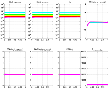
(a) Example (39). Errors, estimator and $\operatorname{IEI}$ are plotted on the top row and $\operatorname{EOC}$s and energy of the reconstructed solution on the bottom row over time ($x$-axis). Results are computed on the sequence of uniform meshes with mesh size $h$, fixed time step $k=0.4h/(p+1)^{2}$ and $p=2$. The $\operatorname{IEI}$ behaviour indicates that the error is well estimated by the estimator and the convergence rate of the estimator remains near to $\operatorname{EOC}\approx 2$, i.e., to that of the errors $e_{L}$ and $e_{R}$.

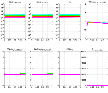
(b) Example (40). Errors, estimator and $\operatorname{IEI}$ are plotted on the top row and $\operatorname{EOC}$s and energy of the reconstructed solution on the bottom row over time ($x$-axis). Results are computed on the sequence of uniform meshes with mesh size $h$, fixed time step $k=0.4h/(p+1)^{2}$ and $p=2$. The $\operatorname{IEI}$ behaviour indicates that the error is well estimated by the estimator and the convergence rate of the estimator remains near to $\operatorname{EOC}\approx 2$, i.e., to that of the errors $e_{L}$ and $e_{R}$.

Fig. 2: Example (41).

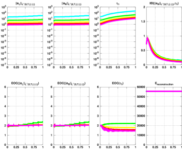
(a) Example (41). Errors, estimator and $\operatorname{IEI}$ are depicted on the top row and $\operatorname{EOC}$s and energy of the reconstructed solution on the bottom row over time ($x$-axis). Results are computed on the sequence of uniform meshes with mesh size $h$, time-step $k=0.1h/(p+1)^{2}$ and $p=2$. The $\operatorname{IEI}$ behaviour indicates that the error is overestimated by the estimator. The convergence rate of the estimator is slightly below $2$, probably due to the somewhat coarse time-step for asymptotic convergence, cf., subfigure (b) below.

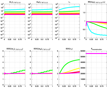
(b) Example (41). Errors, estimator and $\operatorname{IEI}$ are depicted on the top row and $\operatorname{EOC}$s and energy of the reconstructed solution on the bottom row over time ($x$-axis). Results are computed on the sequence of uniform meshes with mesh size $h$, time-step $k=0.4h^{2}/(p+1)^{2}$, and $p=2$. The effect of using slightly smaller time-step for fine $h$ (resulting from the $h^{2}$-term) is evident compared to subfigure (a) above, in that the $\operatorname{EOC}\geq 2$ for all times.

Fig. 3: Example (39), violation of the CFL condition.

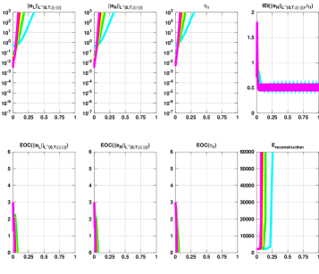
(a) Example (39). Errors, estimator and $\operatorname{IEI}$ are depicted on the top row and $\operatorname{EOC}$s and energy of the reconstructed solution on the bottom row over time ($x$-axis). Results are computed on the sequence of uniform meshes with mesh size $h$ and time step $k=2.0h/(p+1)^{2}$ and $p=3$. The $\operatorname{IEI}$ behaviour indicates that the error is overestimated by the estimator but follows the error behaviour. The method is unstable due to the violation of the CFL condition (cf., Figure 2(b) for comparison with a stable approximation.)

References

- [1] Slimane Adjerid, A posteriori finite element error estimation for second-order hyperbolic problems, Comput. Methods Appl. Mech. Engrg., 191 (2002), pp. 4699–4719.
- [2] Georgios Akrivis, Charalambos Makridakis, and Ricardo H. Nochetto, A posteriori error estimates for the Crank-Nicolson method for parabolic equations, Math. Comp., 75 (2006), pp. 511–531 (electronic).
- [3] , Optimal order a posteriori error estimates for a class of Runge-Kutta and Galerkin methods, Numer. Math., 114 (2009), pp. 133–160.
- [4] , Galerkin and Runge-Kutta methods: unified formulation, a posteriori error estimates and nodal superconvergence, Numer. Math., 118 (2011), pp. 429–456.
- [5] Garth A. Baker, Vassilios A. Dougalis, and Steven M. Serbin, High order accurate two-step approximations for hyperbolic equations, RAIRO Anal. Numér., 13 (1979), pp. 201–226.
- [6] , An approximation theorem for second-order evolution equations, Numer. Math., 35 (1980), pp. 127–142.
- [7] Wolfgang Bangerth and Rolf Rannacher, Adaptive finite element techniques for the acoustic wave equation, J. Comput. Acoust., 9 (2001), pp. 575–591.
- [8] A. Bergam, C. Bernardi, and Z. Mghazli, A posteriori analysis of the finite element discretization of some parabolic equations, Math. Comp., 74 (2005), pp. 1117–1138 (electronic).
- [9] Christine Bernardi and Endre Süli, Time and space adaptivity for the second-order wave equation, Math. Models Methods Appl. Sci., 15 (2005), pp. 199–225.
- [10] Christine Bernardi and Rüdiger Verfürth, A posteriori error analysis of the fully discretized time-dependent Stokes equations, M2AN Math. Model. Numer. Anal., 38 (2004), pp. 437–455.
- [11] M. P. Calvo and J. M. Sanz-Serna, The development of variable-step symplectic integrators, with application to the two-body problem, SIAM J. Sci. Comput., 14 (1993), pp. 936–952.
- [12] Kenneth Eriksson and Claes Johnson, Adaptive finite element methods for parabolic problems. II. Optimal error estimates in and , SIAM J. Numer. Anal., 32 (1995), pp. 706–740.
- [13] Emmanuil H. Georgoulis, Omar Lakkis, and Charalambos Makridakis, A posteriori -error bounds for finite element approximations to the wave equation, IMA J. Numer. Anal., 33 (2013), pp. 1245–1264.
- [14] Ernst Hairer, Christian Lubich, and Gerhard Wanner, Geometric numerical integration illustrated by the Störmer-Verlet method, Acta Numer., 12 (2003), pp. 399–450.
- [15] Paul Houston and Endre Süli, Adaptive Lagrange-Galerkin methods for unsteady convection-diffusion problems, Math. Comp., 70 (2001), pp. 77–106.
- [16] Claes Johnson, Discontinuous Galerkin finite element methods for second order hyperbolic problems, Comput. Methods Appl. Mech. Engrg., 107 (1993), pp. 117–129.
- [17] Omar Lakkis and Charalambos Makridakis, Elliptic reconstruction and a posteriori error estimates for fully discrete linear parabolic problems, Math. Comp., 75 (2006), pp. 1627–1658 (electronic).
- [18] Christian Lubich and Charalambos Makridakis, Interior a posteriori error estimates for time discrete approximations of parabolic problems, Numer. Math., 124 (2013), pp. 541–557.
- [19] Charalambos Makridakis and Ricardo H. Nochetto, Elliptic reconstruction and a posteriori error estimates for parabolic problems, SIAM J. Numer. Anal., 41 (2003), pp. 1585–1594 (electronic).
- [20] , A posteriori error analysis for higher order dissipative methods for evolution problems, Numer. Math., 104 (2006), pp. 489–514.
- [21] Marco Picasso, Adaptive finite elements for a linear parabolic problem, Comput. Methods Appl. Mech. Engrg., 167 (1998), pp. 223–237.
- [22] Robert D. Skeel, Variable step size destabilizes the Störmer/leapfrog/Verlet method, BIT, 33 (1993), pp. 172–175.
- [23] E. Süli, A posteriori error analysis and global error control for adaptive finite volume approximations of hyperbolic problems, in Numerical analysis 1995 (Dundee, 1995), vol. 344 of Pitman Res. Notes Math. Ser., Longman, Harlow, 1996, pp. 169–190.
- [24] Endre Süli, A posteriori error analysis and adaptivity for finite element approximations of hyperbolic problems, in An introduction to recent developments in theory and numerics for conservation laws (Freiburg/Littenweiler, 1997), vol. 5 of Lect. Notes Comput. Sci. Eng., Springer, Berlin, 1999, pp. 123–194.
- [25] R. Verfürth, A posteriori error estimates for finite element discretizations of the heat equation, Calcolo, 40 (2003), pp. 195–212.