Abstract

We present two maximally superintegrable Hamiltonian systems ${\cal H}_{\lambda}$ and ${\cal H}_{\eta}$ that are defined, respectively, on an $N$-dimensional spherically symmetric generalization of the Darboux surface of type III and on an $N$-dimensional Taub–NUT space. Afterwards, we show that the quantization of ${\cal H}_{\lambda}$ and ${\cal H}_{\eta}$ leads, respectively, to exactly solvable deformations (with parameters $\lambda$ and $\eta$) of the two basic quantum mechanical systems: the harmonic oscillator and the Coulomb problem. In both cases the quantization is performed in such a way that the maximal superintegrability of the classical Hamiltonian is fully preserved. In particular, we prove that this strong condition is fulfilled by applying the so-called conformal Laplace–Beltrami quantization prescription, where the conformal Laplacian operator contains the usual Laplace–Beltrami operator on the underlying manifold plus a term proportional to its scalar curvature (which in both cases has non-constant value). In this way, the eigenvalue problems for the quantum counterparts of ${\cal H}_{\lambda}$ and ${\cal H}_{\eta}$ can be rigorously solved, and it is found that their discrete spectrum is just a smooth deformation (in terms of the parameters $\lambda$ and $\eta$) of the oscillator and Coulomb spectrum, respectively. Moreover, it turns out that the maximal degeneracy of both systems is preserved under deformation. Finally, new further multiparametric generalizations of both systems that preserve their superintegrability are envisaged.

1 Introduction

It is well known that if we consider a natural classical Hamiltonian system on the $N$-dimensional ($N$D) Euclidean space

$${\cal H}={\cal T}(\mathbf{p})+{\cal U}(\mathbf{q}),$$ (1)

the harmonic oscillator potential ${\cal U}(\mathbf{q})=\omega^{2}\mathbf{q}^{2}$ and the Coulomb potential ${\cal U}(\mathbf{q})=-k/|\mathbf{q}|$ define two maximally superintegrable (MS) systems (in the Liouville sense), since both systems are endowed with $(2N-1)$ functionally independent and globally defined integrals of the motion. In the first case such integrals are provided by the components of the Demkov–Fradkin tensor [1, 2], and in the second one by the angular momenta together with the $N$ components of the Runge–Lenz vector (see e.g. [3] and references therein). At the classical dynamical level, the footprint of superintegrability consists in the fact that all bounded trajectories of these two systems are closed ones, a fact which is diretly related with Bertrand’s theorem [4]. Moreover, when the quantization of these systems is performed it is found that such superintegrability implies that their spectrum exhibits maximal degeneracy due to a superabundance of quantum integrals of the motion.

In this paper we review two spherically symmetric deformations of the oscillator and Coulomb systems that define two new MS systems [5, 6]. As a consequence, their quantization [7, 8, 9] is shown to present maximal degeneracy in the spectra. At a first sight, the existence of such deformations could seem impossible since the only spherically symmetric potentials on the Euclidean space that are MS are just the oscillator and the Coulomb ones. Therefore, the addition of any radial perturbation on these systems leads to superintegrability breaking and thus to a lack of maximal degeneracy in the spectra, a fact that is very well known in quantum perturbation theory. However, as we shall see, such superintegrable perturbations can be obtained if both the potential and the kinetic energy are simultaneously deformed in a very precise way. Explicitly, the Hamiltonian (1) will be smoothly deformed into

$${\cal H}_{\mu}(\mathbf{q},\mathbf{p})={\cal T}_{\mu}(\mathbf{q},\mathbf{p})+{\cal U}_{\mu}(\mathbf{q}),$$ (2)

where $\mu$ can be regarded as a (generic) deformation parameter in such a manner that we will be no longer working on the flat Euclidean space, but on a suitable curved space with metric and kinetic energy given by

$${\rm d}s_{\mu}^{2}=\sum_{i,j=1}^{N}g_{ij}(\mathbf{q}){\rm d}q_{i}{\rm d}q_{j},\quad\ {\cal T}_{\mu}(\mathbf{q},\mathbf{p})=\frac{1}{2}\sum_{i,j=1}^{N}g^{ij}(\mathbf{q}){p_{i}p_{j}}.$$

This fact will provide additional interesting geometric features to the systems we will deal with. In particular, we will see that the curved/deformed generalization of the Demkov–Fradkin tensor and of the Runge–Lenz vector do exist, and will be the essential tool to prove the MS property of the deformed systems.

We recall that the quantization problem on curved spaces is clearly a non-trivial one, since the kinetic energy term ${\cal T}_{\mu}(\mathbf{q},\mathbf{p})$ is a function of both positions and momenta that creates severe ordering ambiguities. Nevertheless, we shall explicitly show that a quantization of ${\cal{H}}_{\mu}$ (2) that preserves the MS property is achieved through the conformal Laplacian quantization (see [8, 9, 10, 11, 12, 13] and references therein):

$$\hat{\mathcal{H}}_{\rm c,\mu}=\hat{\mathcal{T}}_{\rm c,\mu}+{\mathcal{U}}_{\mu}=-\frac{\hbar^{2}}{2}\Delta_{\rm c,\mu}+{\mathcal{U}}_{\mu}=-\frac{\hbar^{2}}{2}\left(\Delta_{\rm LB,\mu}-\frac{(N-2)}{4(N-1)}\,R_{\mu}\right)+\mathcal{U}_{\mu}\,,$$ (3)

where $R_{\mu}$ is the scalar curvature on the underlying $N$D curved manifold ${\cal M}_{\mu}$, the operator $\Delta_{\rm c,\mu}$ is the conformal Laplacian [14] and $\Delta_{\rm LB,\mu}$ is the usual Laplace–Beltrami operator on ${\cal M}_{\mu}$, i.e.,

$$\Delta_{\rm LB,\mu}=\sum_{i,j=1}^{N}\frac{1}{\sqrt{g}}\partial_{i}\sqrt{g}g^{ij}\partial_{j}\,,$$

where $g^{ij}$ is the inverse of the metric tensor $g_{ij}$ and $g$ is the corresponding determinant. The limit $\mu\to 0$ gives rise to the quantization of the flat Hamiltonian (1) with ${\rm d}s^{2}={\rm d}\mathbf{q}^{2}$ since

$$\lim_{\mu\to 0}R_{\mu}=0,\qquad\lim_{\mu\to 0}\Delta_{\rm c,\mu}=\lim_{\mu\to 0}\Delta_{\rm LB,\mu}=\Delta=\nabla^{2},\qquad\lim_{\mu\to 0}\hat{\mathcal{H}}_{\rm c,\mu}=-\frac{\hbar^{2}}{2}\nabla^{2}+{\mathcal{U}}\,.$$

We also recall that the quantization (3) can be related through a similarity transformation to the Hamiltonian obtained by means of the so-called direct Schrödinger quantization prescription on conformally flat spaces [7, 8]

$$\hat{\mathcal{H}}_{\mu}=\hat{\mathcal{T}}_{\mu}+{\mathcal{U}}_{\mu}=-\frac{\hbar^{2}}{2f_{\mu}(r)^{2}}\,\Delta+\mathcal{U}_{\mu}\,,$$

where $f_{\mu}(r)=f_{\mu}(|\mathbf{q}|)$ is the conformal factor of the metric on ${\cal M}_{\mu}$ written as ${\rm d}s_{\mu}^{2}=f_{\mu}(r)^{2}{\rm d}\mathbf{q}^{2}$. In this case, the scalar curvature reads

$$R_{\mu}=-(N-1)\left(\frac{(N-4)f_{\mu}^{\prime}(r)^{2}+f_{\mu}(r)\left(2f_{\mu}^{\prime\prime}(r)+2(N-1)r^{-1}f_{\mu}^{\prime}(r)\right)}{f_{\mu}(r)^{4}}\right).$$ (4)

In the next two sections, we review the exactly solvable deformations of the $N$D isotropic oscillator $\hat{\mathcal{H}}_{\rm c,\lambda}$ [8] and the Coulomb system $\hat{\mathcal{H}}_{\rm c,\eta}$ [9], correspondingly. New results are sketched in the last section by presenting the only possible multiparametric spherically symmetric generalizations of the above systems which are MS with quadratic integrals of motion, that is, the most generic deformations that can be endowed, respectively, with a generalized Demkov–Fradkin tensor and with a Runge–Lenz $N$-vector.

2 An exactly solvable deformation of the oscillator system

The $N$D classical Hamiltonian system given by

$${\cal H}_{\lambda}(\mathbf{q},\mathbf{p})={\cal T}_{\lambda}(\mathbf{q},\mathbf{p})+{\cal U}_{\lambda}(\mathbf{q})=\frac{\mathbf{p}^{2}}{2(1+\lambda\mathbf{q}^{2})}+\frac{\omega^{2}\mathbf{q}^{2}}{2(1+\lambda\mathbf{q}^{2})},$$ (5)

where $\lambda$ and $\omega$ are real parameters and $\mathbf{q},\mathbf{p}\in\mathbb{R}^{N}$ are canonical coordinates and momenta, was proven in [5] to be MS. The kinetic energy ${\cal T}_{\lambda}(\mathbf{q},\mathbf{p})$ can be interpreted as the one generating the geodesic motion of a particle with unit mass on a conformally flat space with metric and (non-constant) scalar curvature (4) given by

$${\rm d}s_{\lambda}^{2}=(1+\lambda\mathbf{q}^{2}){\rm d}\mathbf{q}^{2},\qquad R_{\lambda}(\mathbf{q})=-\lambda\,\frac{(N-1)\bigl{(}2N+3\lambda(N-2)\mathbf{q}^{2}\bigr{)}}{(1+\lambda\mathbf{q}^{2})^{3}}.$$

Such a curved space is, in fact, an $N$D spherically symmetric generalization ${\mathcal{M}}_{\lambda}$ [15, 16] of the Darboux surface of type III [17, 18, 19]. The limit $\lambda\to 0$ of the above expressions leads to the well known results concerning the (flat) $N$D isotropic harmonic oscillator with frequency $\omega$:

$${\cal H}=\frac{1}{2}\mathbf{p}^{2}+\frac{1}{2}\omega^{2}\mathbf{q}^{2},\qquad{\rm d}s^{2}={\rm d}\mathbf{q}^{2},\qquad R=0.$$

The remarkable point is that ${\cal H}_{\lambda}$ is a MS Hamiltonian, a fact that can be stated as follows.

Proposition 1. [5, 6] (i) The Hamiltonian ${\cal H}_{\lambda}$ (5) is endowed with the following constants of motion ($m=2,\dots,N$):

$\bullet$ $(2N-3)$ angular momentum integrals:

$$C^{(m)}=\!\!\sum_{1\leq i<j\leq m}\!\!\!\!(q_{i}p_{j}-q_{j}p_{i})^{2},\qquad C_{(m)}=\!\!\!\sum_{N-m<i<j\leq N}\!\!\!\!\!\!(q_{i}p_{j}-q_{j}p_{i})^{2},\qquad C^{(N)}=C_{(N)}.$$ (6)

$\bullet$ $N^{2}$ integrals which form the ND curved/deformed Demkov–Fradkin tensor ($i,j=1,\dots,N$):

$$I_{\lambda,ij}=p_{i}p_{j}-\bigl{(}2\lambda{\cal H}_{\lambda}(\mathbf{q},\mathbf{p})-\omega^{2}\bigr{)}q_{i}q_{j},\qquad{\cal H}_{\lambda}=\frac{1}{2}\sum_{i=1}^{N}I_{\lambda,ii}\,.$$

(ii) Each of the three sets $\{{\cal H}_{\lambda},C^{(m)}\}$, $\{{\cal H}_{\lambda},C_{(m)}\}$ ($m=2,\dots,N$) and $\{I_{\lambda,ii}\}$ ($i=1,\dots,N$) is formed by $N$ functionally independent functions in involution.

(iii) The set $\{{\cal H}_{\lambda},C^{(m)},C_{(m)},I_{\lambda,ii}\}$ for $m=2,\dots,N$ with a fixed index $i$ is constituted by $(2N-1)$ functionally independent functions.

Let us now consider the standard definitions for the quantum positions $\hat{\mathbf{q}}=(\hat{q}_{1},\dots,\hat{q}_{N})$, momenta $\hat{\mathbf{p}}=(\hat{p}_{1},\dots,\hat{p}_{N})$ and $\nabla=(\frac{\partial}{\partial q_{1}},\dots,\frac{\partial}{\partial q_{N}})$ operators ($i,j=1,\dots,N)$:

$$\hat{q}_{i}\,\psi(\mathbf{q})=q_{i}\,\psi(\mathbf{q}),\qquad\hat{p}_{i}\,\psi(\mathbf{q})=-{\rm i}\hbar\,\frac{\partial\,\psi(\mathbf{q})}{\partial q_{i}},\qquad[\hat{q}_{i},\hat{p}_{j}]={\rm i}\hbar\,\delta_{ij},\qquad\mathbf{q}\cdot\nabla=\sum_{i=1}^{N}q_{i}\frac{\partial}{\partial q_{i}}\,.$$

If we now apply the conformal Laplacian quantization prescription (3) to ${\cal H}_{\lambda}$ (5) we find:

Proposition 2. [8] Let $\hat{\cal H}_{{\rm c},\lambda}$ be the quantum Hamiltonian given by

$$\hat{\cal H}_{{\rm c},\lambda} =-\frac{\hbar^{2}}{2}\Delta_{\rm LB,\lambda}+\frac{\omega^{2}\mathbf{q}^{2}}{2(1+\lambda\mathbf{q}^{2})}-{\hbar^{2}\lambda(N-2)}\left(\frac{2N+3\lambda(N-2)\mathbf{q}^{2}}{8(1+\lambda{\mathbf{q}}^{2})^{3}}\right)\,,$$

$$\mbox{with}\qquad\Delta_{\rm LB,\lambda}=\frac{1}{(1+\lambda\mathbf{q}^{2})}\,\Delta+\frac{\lambda(N-2)}{(1+\lambda\mathbf{q}^{2})^{2}}\,(\mathbf{q}\cdot\nabla)\,.$$ (7)

(i) $\hat{\cal H}_{{\rm c},\lambda}$ commutes with the $(2N-3)$ quantum angular momentum operators $(m=2,\dots,N)$

$$\hat{C}^{(m)}=\!\!\sum_{1\leq i<j\leq m}\!\!\!\!(\hat{q}_{i}\hat{p}_{j}-\hat{q}_{j}\hat{p}_{i})^{2},\qquad\hat{C}_{(m)}=\!\!\!\sum_{N-m<i<j\leq N}\!\!\!\!\!\!(\hat{q}_{i}\hat{p}_{j}-\hat{q}_{j}\hat{p}_{i})^{2},\qquad\hat{C}^{(N)}=\hat{C}_{(N)}\,,$$ (8)

as well as with the $N^{2}$ curved/deformed Demkov–Fradkin operators given by

$$\hat{I}_{{\rm c},\lambda,ij}=\hat{p}_{i}\hat{p}_{j}-(N-2)\frac{{\rm i}\hbar\lambda}{2(1+\lambda\hat{\mathbf{q}}^{2})}\,(\hat{q}_{i}\hat{p}_{j}+\hat{q}_{j}\hat{p}_{i})+\frac{(N-2)\hbar^{2}\lambda^{2}\hat{q}_{i}\hat{q}_{j}}{(1+\lambda\hat{\mathbf{q}}^{2})^{2}}\left(1-\frac{N-2}{4}\right)$$

$$\qquad\quad\qquad-\frac{(N-2)\hbar^{2}\lambda}{2(1+\lambda\hat{\mathbf{q}}^{2})}\,\delta_{ij}-2\lambda\hat{q}_{i}\hat{q}_{j}{\hat{\cal H}_{{\rm c},\lambda}}(\hat{\mathbf{q}},\hat{\mathbf{p}})+\omega^{2}\hat{q}_{i}\hat{q}_{j},$$

with $i,j=1,\dots,N$ and such that ${\hat{\cal H}_{{\rm c},\lambda}}=\frac{1}{2}\sum_{i=1}^{N}\hat{I}_{{\rm c},\lambda,ii}$.

(ii) Each of the three sets $\{{\hat{\cal H}_{{\rm c},\lambda}},\hat{C}^{(m)}\}$, $\{{\hat{\cal H}_{{\rm c},\lambda}},\hat{C}_{(m)}\}$ ($m=2,\dots,N$) and $\{\hat{I}_{{\rm c},\lambda,ii}\}$ ($i=1,\dots,N$) is formed by $N$ algebraically independent commuting observables.

(iii) The set $\{{\hat{\cal H}_{{\rm c},\lambda}},\hat{C}^{(m)},\hat{C}_{(m)},\hat{I}_{{\rm c},\lambda,ii}\}$ for $m=2,\dots,N$ with a fixed index $i$ is formed by $(2N-1)$ algebraically independent observables.

(iv) $\hat{\cal H}_{{\rm c},\lambda}$ is formally self-adjoint on the space $L^{2}({\mathcal{M}}_{\lambda})$, associated with the underlying Darboux III space, defined by

$$\langle\Psi|\Phi\rangle_{\rm c,\lambda}=\int_{{\mathcal{M}}_{\lambda}}\overline{{\Psi}(\mathbf{q})}\,\Phi(\mathbf{q})\,(1+\lambda\mathbf{q}^{2})^{N/2}\,{\rm d}\mathbf{q}.$$

The complete solution to the eigenvalue problem along with the corresponding eigenfunctions for the case of positive deformation parameter $\lambda$ is summarized in the following statement.

Theorem 3. [8] Let $\hat{\cal H}_{{\rm c},\lambda}$ be the quantum Hamiltonian (7) with $\lambda>0$. Then:

(i) The continuous spectrum of $\hat{\cal H}_{{\rm c},\lambda}$ is given by $[\frac{\omega^{2}}{2\lambda},\infty)$. There are no embedded eigenvalues and its singular spectrum is empty.

(ii) $\hat{\cal H}_{{\rm c},\lambda}$ has an infinite number of eigenvalues, all of which are contained in $(0,\frac{\omega^{2}}{2\lambda})$. Their only accumulation point is $\frac{\omega^{2}}{2\lambda}$ which is the bottom of the continuous spectrum.

(iii) All the discrete eigenvalues of $\hat{\cal H}_{{\rm c},\lambda}$ are of the form

$$E_{\lambda,n}\!\!\! = \!\!\!-\lambda\hbar^{2}\left(n+\frac{N}{2}\right)^{2}+\hbar\left(n+\frac{N}{2}\right)\sqrt{\hbar^{2}\lambda^{2}\left(n+\frac{N}{2}\right)^{2}+\omega^{2}},\qquad n\in\mathbb{N}\,.$$ (9)

(iv) The eigenfunction $\Psi_{{\rm c},\lambda}$ of $\hat{\cal H}_{{\rm c},\lambda}$ with eigenvalue $E_{\lambda,n}$ is given by

$$\Psi_{{\rm c},\lambda}(\mathbf{q})=(1+\lambda\mathbf{q}^{2})^{(2-N)/4}\prod_{i=1}^{N}\exp\{-\beta^{2}q_{i}^{2}/2\}H_{n_{i}}(\beta q_{i}),\qquad\beta=\sqrt{\frac{\Omega}{\hbar}},$$

where $H_{n_{i}}$ are Hermite polynomials with $n_{i}\in\mathbb{N}$ such that $n_{1}+\cdots+n_{N}=n$ and the deformed frequency $\Omega$ is defined by

$$\Omega=\sqrt{\omega^{2}-2\lambda E_{\lambda,n}}\,.$$

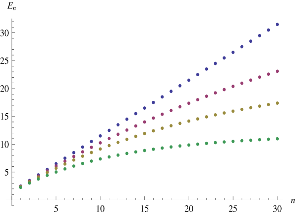
Figure 1: The discrete spectrum $E_{\lambda,n}$ (9) for $0\leq n\leq 25$, $N=3$, $\hbar=\omega=1$ and $\lambda=\{0,0.01,0.02,0.04\}$ starting from the upper dot (straight) line corresponding to the isotropic harmonic oscillator with $\lambda=0$, that is, $E_{0,n}$. In the same order, $E_{\lambda,0}=\{1.5,1.48,1.46,1.41\}$ and $E_{\lambda,\infty}=\{\infty,50,25,12.5\}$.

Moreover, the bound states of this system satisfy

$$E_{\lambda,\infty}=\lim_{n\to\infty}E_{\lambda,n}=\frac{\omega^{2}}{2\lambda},\qquad\lim_{n\to\infty}(E_{\lambda,n+1}-E_{\lambda,n})=0.$$

The discrete spectrum (9) is depicted in figure 1 as a function of $n$ for several values of $\lambda$. As it was remarked in the introduction, the spectrum turns out to be maximally degenerate since it can be described as a function of just one quantum number $n\in\mathbb{N}$. By taking into account the definition of $n$, the number of degenerate states $D(E_{\lambda,n})$ for a given energy level $E_{\lambda,n}$ corresponds to all the possible combinations of $\{n_{i}\in\mathbb{N}\}$ obeying to the constraint $\sum_{i=1}^{N}n_{i}=n$, namely

$$D(E_{\lambda,n})=\frac{(n+N-1)!}{n!(N-1)!},$$

which for $N=3$ reduces to the well known expression $D(E_{\lambda,n})={(n+2)(n+1)}/{2}$ for the degeneracies of the isotropic oscillator. Therefore, the curved system has a similar set of integrals of the motion as the undeformed one and, as a consequence, it exhibits the same degeneracy.

3 An exactly solvable deformation of the Coulomb system

Now we consider the $N$D Hamiltonian system given by

$${\cal{H}}_{\eta}={\cal T}_{\eta}(\mathbf{q},\mathbf{p})+{\cal U}_{\eta}(\mathbf{q})=\frac{|\mathbf{q}|}{2(\eta+|\mathbf{q}|)}\,\mathbf{p}^{2}-\frac{k}{\eta+|\mathbf{q}|}\,,$$ (10)

where $\eta$ and $k$ are real parameters. The metric and scalar curvature of the underlying manifold ${\mathcal{M}}_{\eta}$ turns out to be

$${\rm d}s_{\eta}^{2}=\left(1+\frac{\eta}{|\mathbf{q}|}\right){\rm d}\mathbf{q}^{2},\qquad R_{\eta}=\eta(N-1)\,\frac{4(N-3)r+3\eta(N-2)}{4r(\eta+r)^{3}},\qquad r=|\mathbf{q}|=\sqrt{\mathbf{q}^{2}}\,.$$

We remark that the system (10) is directly related to a reduction [20] of the geodesic motion on the Taub–NUT space [21, 22, 23, 24, 25, 26, 27, 28, 29, 30, 31]. In fact, this system can be regarded as an $\eta$-deformation of the $N$D Euclidean Coulomb problem with coupling constant $k$, since the limit $\eta\to 0$ yields

$${\cal H}=\frac{1}{2}\,{\mathbf{p}^{2}}-\frac{k}{|\mathbf{q}|},\qquad{\rm d}s^{2}={\rm d}\mathbf{q}^{2},\qquad R=0.$$

Remarkably enough, the Hamiltonian ${\cal{H}}_{\eta}$ turns out to be a MS classical system, and this result can be summarized as follows.

Proposition 4. [6] (i) The Hamiltonian ${\cal{H}}_{\eta}$ (10) is endowed with the $(2N-3)$ angular momentum integrals (6) and Poisson-commutes with the ${\cal R}_{\eta,i}$ components ($i=1,\dots,N$) of the Runge–Lenz $N$-vector given by

$${\cal R}_{\eta,i}=\sum_{j=1}^{N}p_{j}(q_{j}p_{i}-q_{i}p_{j})+\frac{q_{i}}{|\mathbf{q}|}\left(\eta{\cal{H}}_{\eta}(\mathbf{q},\mathbf{p})+k\right).$$

(ii) The set $\{{\cal H}_{\eta},C^{(m)},C_{(m)},{\cal R}_{\eta.{i}}\}$ with $m=2,\dots,N$ and a fixed index $i$ is formed by $(2N-1)$ functionally independent functions.

We also recall that the classical system ${\cal{H}}_{\eta}$ has been fully solved in [32]. Next the quantum counterpart of (10) can be obtained by applying (3), and reads:

Proposition 5. [9] (i) The quantum Hamiltonian $\hat{\cal H}_{{\rm c},\eta}$ given by

$$\hat{\cal H}_{{\rm c},\eta}=-\frac{\hbar^{2}}{2}\Delta_{\rm LB,\eta}-\frac{k}{\eta+|\mathbf{q}|}+\hbar^{2}\eta(N-2)\,\frac{4(N-3)|\mathbf{q}|+3\eta(N-2)}{32|\mathbf{q}|(\eta+|\mathbf{q}|)^{3}}\,,$$

$$\mbox{with}\qquad\Delta_{\rm LB,\eta}=\frac{|\mathbf{q}|}{\eta+|\mathbf{q}|}\,\Delta-\frac{\eta(N-2)}{2|\mathbf{q}|(|\mathbf{q}|+\eta)^{2}}\,(\mathbf{q}\cdot\nabla)\,,$$ (11)

commutes with the $(2N-3)$ quantum angular momentum operators (8) as well as with the following $N$ Runge–Lenz operators $(i=1,\dots,N)$:

$${\normalsize{\hat{\cal R}_{{\rm c},\eta,i}=\frac{1}{2}\sum_{j=1}^{N}\left(\hat{p}_{j}+{\rm i}\hbar\,\eta\,\frac{(N-2)\hat{q}_{j}}{4(\eta+|\hat{\mathbf{q}}|)\,\hat{\mathbf{q}}^{2}}\right)(\hat{q}_{j}\hat{p}_{i}-\hat{q}_{i}\hat{p}_{j})}}$$

$$\qquad\qquad+\frac{1}{2}\sum_{j=1}^{N}(\hat{q}_{j}\hat{p}_{i}-\hat{q}_{i}\hat{p}_{j})\left(\hat{p}_{j}+{\rm i}\hbar\,\eta\,\frac{(N-2)\hat{q}_{j}}{4(\eta+|\hat{\mathbf{q}}|)\,\hat{\mathbf{q}}^{2}}\right)+\frac{\hat{q}_{i}}{|\hat{\mathbf{q}}|}\left(\eta\hat{\cal{H}}_{\rm c,\eta}(\mathbf{q},\mathbf{p})+k\right).$$

(ii) Each of the three sets $\{{\hat{\cal H}_{{\rm c},\eta}},\hat{C}^{(m)}\}$, $\{{\hat{\cal H}_{{\rm c},\eta}},\hat{C}_{(m)}\}$ ($m=2,\dots,N$) and $\{\hat{\cal R}_{{\rm c},\eta,i}\}$ ($i=1,\dots,N$) is formed by $N$ algebraically independent commuting operators.

(iii) The set $\{{\hat{\cal H}_{{\rm c},\eta}},\hat{C}^{(m)},\hat{C}_{(m)},\hat{\cal R}_{{\rm c},\eta,i}\}$ for $m=2,\dots,N$ with a fixed index $i$ is formed by $(2N-1)$ algebraically independent operators.

(iv) $\hat{\cal H}_{{\rm c},\eta}$ is formally self-adjoint on the Hilbert space $L^{2}({\mathcal{M}}_{\eta})$ with the scalar product

$$\langle\Psi|\Phi\rangle_{\rm c,\eta}=\int_{{\mathcal{M}}_{\eta}}\overline{{\Psi}(\mathbf{q})}\,\Phi(\mathbf{q})\,\left(1+\frac{\eta}{|\mathbf{q}|}\right)^{N/2}\,{\rm d}\mathbf{q}.$$

For a positive value of the deformation parameter $\eta$, the complete solution of the eigenvalue problem for this quantum mechanical deformed Coulomb problem is the following.

Theorem 6. [9] Let $\hat{\cal H}_{{\rm c},\eta}$ be the quantum Hamiltonian (11) with $k>0$ and $\eta>0$. Then:

(i) The continuous spectrum of $\hat{\cal H}_{{\rm c},\eta}$ is given by $[0,\infty)$. There are no embedded eigenvalues and the singular spectrum is empty.

(ii) $\hat{\cal H}_{{\rm c},\eta}$ has an infinite number of eigenvalues $E_{\eta,n,l}$, depending only on the sum $(n+l)$ and accumulating at $0$.

(iii) The eigenvalues $E_{\eta,n,l}$ of $\hat{\cal H}_{{\rm c},\eta}$ are of the form

$$E_{\eta,n,l}=\frac{-k^{2}}{\hbar^{2}\left(n+l+\frac{N-1}{2}\right)^{2}+k\eta+\sqrt{\hbar^{4}\left(n+l+\frac{N-1}{2}\right)^{4}+2\,\hbar^{2}k\eta\left(n+l+\frac{N-1}{2}\right)^{2}}}\,,$$ (12)

such that the radial eigenfunction $\Phi_{{\rm c},\eta}(r)$ of $\hat{\cal H}_{{\rm c},\eta}$ with eigenvalue $E_{\eta,n,l}$ reads

$$\Phi_{{\rm c,\eta}}(r)=\left(1+\frac{\eta}{r}\right)^{\frac{2-N}{4}}r^{l}\exp\left(-\frac{Kr}{\hbar^{2}\left(n+l+\frac{N-1}{2}\right)}\right)\,L_{n}^{2l+N-2}\left(\frac{2Kr}{\hbar^{2}\left(n+l+\frac{N-1}{2}\right)}\right),$$

where $L_{n}^{\alpha}$ are generalized Laguerre polynomials and the deformed coupling constant $K$ reads

$$K=k+\eta\,E_{\eta,n,l}.$$

Since $\hat{\cal H}_{{\rm c},\eta}$ is a Hamiltonian with radial symmetry, its complete eigenfunction is so given by $\Psi_{{\rm c},\eta}=\Phi_{{\rm c},\eta}(r)Y_{\boldsymbol{l}}(\boldsymbol{\theta})$ where $Y_{\boldsymbol{l}}(\boldsymbol{\theta})$ denotes the usual hyperspherical harmonics, $\boldsymbol{\theta}=(\theta_{1},\dots,\theta_{N-1})$ and $\boldsymbol{l}$ is a vector of $N-1$ quantum numbers $\boldsymbol{l}=(l_{2},\dots,l_{N-1},l_{N}=l)$ such that (see (8))

$${\hat{C}}^{(m)}Y_{\boldsymbol{l}}(\boldsymbol{\theta})=\hbar^{2}l_{m}(l_{m}+m-2)Y_{\boldsymbol{l}}(\boldsymbol{\theta}),\qquad l_{m}-l_{m-1}\geq 0,\qquad m=2,\dots N.$$

Figure 2: Discrete spectrum (12) for the fundamental and the three first excited states of the Hamiltonian $\hat{\cal H}_{{\rm c},\eta}$ (11) when $\eta=\{0,0.2,0.4,0.6,1\}$ with $\hbar=k=1$ and $N\geq 3$. Note that the effect of the $\eta$ deformation is quite strong for the fundamental state, since it comes from the shift $r\to r+\eta$ in the usual Coulomb potential.

Notice also that the bound states of this system satisfy

$$\lim_{n,l\to\infty}E_{\eta,n,l}=0,\qquad\lim_{\mathfrak{n}\to\infty}(E_{\eta,\mathfrak{n}+1}-E_{\eta,\mathfrak{n}})=0,\qquad\mathfrak{n}=n+l.$$

As expected, the limit $\eta\to 0$ of $E_{\eta,n,l}$ provides the well known formula for the standard Coulomb eigenvalues $E_{0,n,l}$

$$E_{0,n,l}=-\frac{k^{2}}{2\hbar^{2}\left(n+l+\frac{N-1}{2}\right)^{2}}\,.$$

And we find that the perturbative series for the eigenvalues of the deformed system $\hat{\cal H}_{{\rm c},\eta}$ (11) reads

$$E_{\eta,n,l}=E_{0,n,l}+\eta\,\frac{k^{3}}{2\hbar^{4}\left(n+l+\frac{N-1}{2}\right)^{4}}-\eta^{2}\,\frac{5k^{4}}{8\hbar^{6}\left(n+l+\frac{N-1}{2}\right)^{6}}+O(\eta^{3}).$$

In figure 2 the eigenvalues of the fundamental and of the first three excited states are plotted for different values of the deformation parameter $\eta$.

As we can see from (12) the spectrum is maximally degenerate as, again, it depends on a unique principal quantum number $\mathfrak{n}=n+l$. The degeneracy $D(E_{\eta,\mathfrak{n}})$ of a given energy level $E_{\eta,\mathfrak{n}}$ can be computed straightforwardly by taking into account that the cardinality $D(L_{l})$ given by the set of the hyperspherical harmonics $\{Y_{\boldsymbol{l}}(\boldsymbol{\theta})\}$ having the same quantum number $l$ and such that $\hat{C}^{(N)}\{Y_{\boldsymbol{l}}(\boldsymbol{\theta})\}=\hbar^{2}l(l+N-2)\{Y_{\boldsymbol{l}}(\boldsymbol{\theta})\}$ reads [33]

$$D(L_{l})=\frac{(2l+N-2)(l+N-3)!}{l!(N-2)!}\,.$$

From it we obtain that

$$D(E_{\eta,\mathfrak{n}})=\sum_{l=0}^{\mathfrak{n}}D(L_{l})=\frac{(2\mathfrak{n}+N-1)(\mathfrak{n}+N-2)!}{\mathfrak{n}!(N-1)!}.$$

In particular, for $N=3$ we obtain $D(E_{\eta,\mathfrak{n}})=(\mathfrak{n}+1)^{2}$, which coincides with the degeneracy of the energy levels of the undeformed Coulomb problem.

4 Generalization

So far we have reviewed some specific exactly solvable deformations of the oscillator and Coulomb potentials, which can be regarded as the most natural MS deformations beyond constant curvature. Nevertheless, there are more possible generalizations within this framework that preserves the classical MS property and that would lead to other exactly solvable deformed oscillator and Coulomb systems. These arise within the classification of Bertrand Hamiltonians formerly introduced in [34] and further developed in [35, 36, 37]. Such systems are MS and their underlying Bertrand spaces are spherically symmetric ones. If we require to keep quadratic integrals of motion, so generalizing the Demkov–Fradkin tensor and the Runge–Lenz $N$-vector, it can be shown that there only exists one possible generalization of the deformations of the oscillator and Coulomb systems here studied that depends on two deformation parameters.

In particular, the two-parameter MS deformation of the oscillator system turns out to be

$${\cal H}_{\lambda,\xi}(\mathbf{q},\mathbf{p})={\cal T}_{\lambda,\xi}(\mathbf{q},\mathbf{p})+{\cal U}_{\lambda,\xi}(\mathbf{q})=\frac{(1-\xi\mathbf{q}^{4})^{2}\mathbf{p}^{2}}{2(1+\lambda\mathbf{q}^{2}+\xi\mathbf{q}^{4})}+\frac{\omega^{2}\mathbf{q}^{2}}{2(1+\lambda\mathbf{q}^{2}+\xi\mathbf{q}^{4})},$$

where $\xi$ is a real parameter. Obviously, the limit $\xi\to 0$ gives rise to the Hamiltonian ${\cal H}_{\lambda}$ (5) The underlying manifold ${\mathcal{M}}_{\lambda,\xi}$ is endowed with a conformally flat metric given by

$${\rm d}s_{\lambda,\xi}^{2}=\frac{(1+\lambda\mathbf{q}^{2}+\xi\mathbf{q}^{4})}{(1-\xi\mathbf{q}^{4})^{2}}\,{\rm d}\mathbf{q}^{2}.$$

And the corresponding scalar curvature (4) reads

$$R_{\lambda,\xi}(r)=-\frac{(N-1)}{(1+\lambda r^{2}+\xi r^{4})^{3}}\bigg{\{}N\big{(}2+3\lambda r^{2}+6\xi r^{4}+\lambda\xi r^{6}\big{)}\big{(}\lambda+3\lambda\xi r^{4}+2\xi r^{2}(3+\xi r^{4})\big{)}$$

$$\qquad\qquad\qquad\qquad\qquad\qquad-6r^{2}(\lambda^{2}-4\xi)(1-\xi r^{4})^{2}\bigg{\}},$$

where recall that $r=|\mathbf{q}|=\sqrt{\mathbf{q}^{2}}$.

As far as the Coulomb system is concerned, the resulting two-parameter MS deformation is given by

$${\cal{H}}_{\eta,\zeta}={\cal T}_{\eta,\zeta}(\mathbf{q},\mathbf{p})+{\cal U}_{\eta,\zeta}(\mathbf{q})=\frac{(1-\zeta\mathbf{q}^{2})^{2}|\mathbf{q}|}{2(\eta+|\mathbf{q}|+\eta\zeta\mathbf{q}^{2})}\,\mathbf{p}^{2}-\frac{k(1+\zeta\mathbf{q}^{2})}{(\eta+|\mathbf{q}|+\eta\zeta\mathbf{q}^{2})}\,,$$

which generalizes the one-parameter Hamiltonian ${\cal H}_{\eta}$ (10). Hence the metric of the underlying spherically symmetric space ${\mathcal{M}}_{\eta,\zeta}$ and its scalar curvature are found to be

$${\rm d}s_{\eta,\zeta}^{2}=\frac{(\eta+|\mathbf{q}|+\eta\zeta\mathbf{q}^{2})}{(1-\zeta\mathbf{q}^{2})^{2}|\mathbf{q}|}\,{\rm d}\mathbf{q}^{2}\,,$$

$$R_{\eta,\zeta}(r)=-\frac{(N-1)}{4r(\eta+r+\eta\zeta r^{2})^{3}}\bigg{\{}6\eta(1-\zeta r^{2})^{2}\bigg{(}\eta+r\big{(}2+\zeta r(6\eta+r[2+\eta\zeta r])\big{)}\bigg{)}$$

$$\qquad\qquad\qquad-N\big{(}3\eta+r(4+\eta\zeta r[6-\zeta r^{2}])\big{)}\big{(}\eta-\zeta r^{2}(6\eta+r[4+3\eta\zeta r])\big{)}\bigg{\}}.$$

It is worth stressing that ${\mathcal{M}}_{\eta,\zeta}$ turns out to be the $N$D spherically symmetric generalization of the Darboux surface of type IV [17, 18, 19] constructed in [15, 16].

Consequently, by applying the conformal Laplacian quantization (3) to the above two-parameter Hamiltonians, new exactly solvable systems, $\hat{\cal{H}}_{\rm c,\lambda,\xi}$ and $\hat{\cal{H}}_{\rm c,\eta,\zeta}$, would be obtained as deformations of the oscillator and Coulomb systems. Their solution would generalize the results presented in theorems 3 and 6. Work on this line is currently in progress.

References

[1]
Demkov Y N 1959 Soviet Phys. JETP9 63
[2]
Fradkin D M 1965 Amer. J. Phys.33 207
[3]
Ballesteros A, Enciso A, Herranz F J and Ragnisco O 2009 Commun. Math. Phys.290 1033
[4]
Bertrand J 1873 C.R. Acad. Sci. Paris77 849
[5] Ballesteros A, Enciso A, Herranz F J and Ragnisco O 2008 Physica D237 505
[6] Ballesteros A, Enciso A, Herranz F J, Ragnisco O and Riglioni D 2011 SIGMA7 048
[7] Ballesteros A, Enciso A, Herranz F J, Ragnisco O and Riglioni D 2011 Phys. Lett. A375 1431
[8] Ballesteros A, Enciso A, Herranz F J, Ragnisco O and Riglioni D 2011 Ann. Phys. 326 2053
[9] Ballesteros A, Enciso A, Herranz F J, Ragnisco O and Riglioni D 2014 Ann. Phys. 351 540
[10]
Wald R M 1984 General Relativity
(Chicago: The University of Chicago Press)
[11]
Liu Z J and Qian M 1992 Trans. Amer. Math. Soc.331 321
[12]
Landsman N P 1998 Mathematical Topics Between Classical and Quantum Mechanics
(New York: Springer)
[13] Michel J P, Radoux F and Silhan J 2014 SIGMA10 016
[14] Baer C and Dahl M 2003 Geom. Funct. Anal.13 483
[15] Ballesteros A, Herranz F J and Ragnisco O 2007 Phys. Lett. B652 376
[16] Ballesteros A, Enciso A, Herranz F J and Ragnisco O 2009 Ann. Phys. 324 1219
[17]
Koenigs G 1972 Leçons sur la thèorie gènèrale des surfaces
vol 4 ed G Darboux (New York: Chelsea) p 368
[18]
Kalnins E G, Kress J M, Miller W Jr and Winternitz P 2003
J. Math. Phys.44 5811
[19] Grosche C, Pogosyan G S and Sissakian A N 2007
Phys. Part. Nuclei38 525
[20]
Iwai T and Katayama N 1994 J. Phys. A: Math. Gen.27 3179
[21]
Manton N S 1982 Phys. Lett. B110 54
[22]
Atiyah M F and Hitchin N J 1985 Phys. Lett. A107 21
[23]
Gibbons G W and Manton N S 1986 Nucl. Phys. B274 183
[24]
Fehér L G and Horváthy P A 1987 Phys. Lett. B183 182
[25]
Gibbons G W and Ruback P J 1988 Comm. Math. Phys.115 267
[26]
Iwai T and Katayama N 1995 J. Math. Phys.36 1790
[27]
Iwai T, Uwano Y and Katayama N 1996 J. Math. Phys.37 608
[28] Bini D, Cherubini C and Jantzen R T 2002 Class. Quantum Grav.19 5481
[29] Bini D, Cherubini C, Jantzen R T and Mashhoon B 2003 Class. Quantum Grav.20 457
[30]
Gibbons G W and Warnick C M 2007 J. Geom. Phys.57 2286
[31] Jezierski J and Lukasik M 2007 Class. Quantum Grav.24 1331
[32]
Latini D and Ragnisco O 2014 preprint arXiv:1411.3571
[33] Atkinson K and Han W 2012
Spherical Harmonics and Approximations on the Unit Sphere: An IntroductionLecture Notes in Mathematics2044 (New York: Springer) p 16
[34]
Perlick V 1992 Class. Quantum Grav.9 1009
[35]
Ballesteros A, Enciso A, Herranz F J and Ragnisco O 2008 Class. Quantum Grav.25 165005
[36] Riglioni D 2013 J. Phys. A: Math. Theor.46 265207
[37] Post S and Riglioni D 2014 preprint arXiv:1410.4495