Large-scale Binary Quadratic Optimization Using Semidefinite Relaxation and Applications

Abstract

In computer vision, many problems can be formulated as binary quadratic programs (BQPs), which are in general NP hard. Finding a solution when the problem is of large size to be of practical interest typically requires relaxation. Semidefinite relaxation usually yields tight bounds, but its computational complexity is high. In this work, we present a semidefinite programming (SDP) formulation for BQPs, with two desirable properties. First, it produces similar bounds to the standard SDP formulation. Second, compared with the conventional SDP formulation, the proposed SDP formulation leads to a considerably more efficient and scalable dual optimization approach. We then propose two solvers, namely, quasi-Newton and smoothing Newton methods, for the simplified dual problem. Both of them are significantly more efficient than standard interior-point methods. Empirically the smoothing Newton solver is faster than the quasi-Newton solver for dense or medium-sized problems, while the quasi-Newton solver is preferable for large sparse/structured problems.

1 Introduction

Binary quadratic programs (BQPs) are a class of combinatorial optimization problems with binary variables, quadratic objective function and linear/quadratic constraints. They appear in a wide variety of applications in computer vision, such as image segmentation/pixel labelling, image registration/matching, image denoising/restoration. Moreover, Maximum a Posteriori (MAP) inference problems for Markov Random Fields (MRFs) can be formulated as BQPs too. There are a long list of references to applications formulated as BQPs or specifically MRF-MAP problems. Readers may refer to [1, 2, 3, 4, 5, 6] and the references therein for detailed studies.

Unconstrained BQPs with submodular pairwise terms can be solved exactly and efficiently using graph cuts [7, 8, 9]. However solving general BQP problems is known to be NP-hard (see [10] for exceptions). In other words, it is unlikely to find polynomial time algorithms to exactly solve these problems. Alternatively, relaxation approaches can be used to produce a feasible solution close to the global optimum in polynomial time. In order to accept such a relaxation we require a guarantee that the divergence between the solutions to the original problem and the relaxed problem is bounded. The quality of the relaxation thus depends upon the tightness of the bounds. Developing an efficient relaxation algorithm with a tight relaxation bound that can achieve a good solution (particularly for large problems) is thus of great practical importance. There are a number of relaxation methods for BQPs (in particular MRF-MAP inference problems) in the literature, including linear programming (LP) relaxation [11, 12, 13, 14], quadratic programming relaxation  [15], second order cone relaxation [16, 17, 18], spectral relaxation [19, 20, 21, 22] and SDP relaxation [17, 23].

Spectral methods are effective for many computer vision applications, such as image segmentation [19, 20] and motion segmentation [24]. The optimization of spectral methods eventually lead to the computation of top eigenvectors. Nevertheless, spectral methods may produce loose relaxation bounds in many cases [25, 26, 27]. Moreover, the inherent quadratic programming formulation of spectral methods is difficult to incorporate certain types of additional constraints [21].

SDP relaxation has been shown that it leads to tighter approximation than other relaxation methods for many combinatorial optimization problems [28, 29, 30, 31]. In particular for the max-cut problem, Goemans and Williamson [32] achieve the state-of-the-art $0.879$ approximation ratio using SDP relaxation. SDP relaxation has also been used in a range of vision problems, such as image segmentation [33], restoration [34, 35], graph matching [36, 37] and co-segmentation [38]. In a standard SDP problem, a linear function of a symmetric matrix $\mathbf{X}$ is optimized, subject to linear (in)equality constraints and the constraint of $\mathbf{X}$ being positive semidefinite (p.s.d.). The standard SDP problem and its Lagrangian dual problem are written as:

$$\mbox{(SDP-P) \quad}\min_{\mathbf{X}\in\mathcal{S}^{n}_{+}} \quad\mathrm{p}(\mathbf{X}):=\langle\mathbf{X},\mathbf{A}\rangle,$$ (1)

$$\mathrm{s.t.}\,\, \quad\langle\mathbf{X},\mathbf{B}_{i}\rangle=b_{i},\ i\in\mathcal{I}_{eq},$$

$$\quad\langle\mathbf{X},\mathbf{B}_{i}\rangle\leq b_{i},\ i\in\mathcal{I}_{in},$$

$$\mbox{(SDP-D) \quad}\max_{\mathbf{u}\in\mathbb{R}^{m}} \quad\mathrm{d}(\mathbf{u}):=-\mathbf{u}^{\!\top}\mathbf{b},$$ (2)

$$\mathrm{s.t.}\,\, \quad\mathbf{A}+\textstyle{\sum_{i=1}^{m}}u_{i}\mathbf{B}_{i}\in\mathcal{S}^{n}_{+},$$

$$\quad u_{i}\geq 0,\ i\in\mathcal{I}_{in},$$

where $m=|\mathcal{I}_{eq}|+|\mathcal{I}_{in}|$, and $\mathcal{I}_{eq}$ ($\mathcal{I}_{in}$) denotes the indexes of linear (in)equality constraints. The p.s.d. constraint $\mathbf{X}\in\mathcal{S}^{n}_{+}$ is convex, so SDP problems are convex optimization problems and the above two formulations are equivalent if a feasible solution exists. The SDP problem (1) can be considered as a semi-infinite LP problem, as the p.s.d. constraint can be converted to an infinite number of linear constraints: $\langle\mathbf{X},\mathbf{a}\mathbf{a}^{\!\top}\rangle\geq 0,\forall\mathbf{a}\in\mathbb{R}^{n}$. Through SDP, these infinite number of linear constraints can be handled in finite time.

It is widely accepted that interior-point methods [39, 40] are very robust and accurate for general SDP problems up to a moderate size (see SeDuMi [41], SDPT3 [42] and MOSEK [43] for implementations). However, its high computational complexity and memory requirement hampers the application of SDP methods to large-scale problems. Approximate nonlinear programming methods [44, 45, 46] are proposed for SDP problems based on low-rank factorization, which may converge to a local optimum. Augmented Lagrangian methods [47, 48] and the variants [49, 50] have also been developed. As gradient-descend based methods [51], they may converge slowly. The spectral bundle method [52] and the log-barrier algorithm [53] can be used for large-scale problems as well. A drawback is that they can fail to solve some SDP problems to satisfactory accuracies [48].

In this work, we propose a regularized SDP relaxation approach to BQPs. Preliminary results of this paper appeared in [54]. Our main contributions are as follows.

1. Instead of directly solving the standard SDP relaxation to BQPs, we propose a quadratically regularized version of the original SDP formulation, which can be solved efficiently and achieve a solution quality comparable to the standard SDP relaxation.

2. We proffer two algorithms to solve the dual problem, based on quasi-Newton (referred to as SDCut-QN) and smoothing Newton (referred to as SDCut-SN) methods respectively. The sparse or low-rank structure of specific problems are also exploited to speed up the computation. The proposed solvers require much lower computational cost and storage memory than standard interior-point methods. In particular, SDCut-QN has a lower computational cost in each iteration while needs more iterations to converge. On the other hand, SDCut-SN converges quadratically with higher computational complexity per iteration. In our experiments, SDCut-SN is faster for dense or medium-sized problems, and SDCut-QN is more efficient for large-scale sparse/structured problems.

3. We demonstrate the efficiency and flexibility of our proposed algorithms by applying them to a variety of computer vision tasks. We show that due to the capability of accommodating various constraints, our methods can encode problem-dependent information. More specifically, the formulation of SDCut allows multiple additional linear and quadratic constraints, which enables a broader set of applications than what spectral methods and graph-cut methods can be applied to.

Notation A matrix (column vector) is denoted by a bold capital (lower-case) letter. $\mathbb{R}^{n}$ denotes the space of real-valued $n\times 1$ vectors. $\mathbb{R}^{n}_{+}$ and $\mathbb{R}^{n}_{-}$ represent the non-negative and non-positive orthants of $\mathbb{R}^{n}$ respectively. $\mathcal{S}^{n}$ denotes the space of $n\times n$ symmetric matrices, and $\mathcal{S}^{n}_{+}$ represents the corresponding cone of positive semidefinite (p.s.d.) matrices. For two vectors, $\mathbf{x}\leq\mathbf{y}$ indicates the element-wise inequality; $\mathrm{trace}(\mathbf{X})$, $\mathrm{rank}(\mathbf{X})$ and $\mathrm{diag}(\mathbf{X})$ denote the trace, rank and the main diagonal elements of $\mathbf{X}$ respectively. $\mathrm{Diag}(\mathbf{x})$ denotes a diagonal matrix with the elements of vector $\mathbf{x}$ on the main diagonal. $\lVert\mathbf{X}\rVert_{F}^{2}$ denotes the Frobenius norm of $\mathbf{X}$. The inner product of two matrices is defined as $\langle\mathbf{X},\mathbf{Y}\rangle$. $\mathbf{I}_{n}$ indicates the $n\times n$ identity matrix. $\mathbf{0}$ and $\mathbf{1}$ denote all-zero and all-one column vectors respectively.$\nabla\mathrm{f}(\cdot)$ and $\nabla^{2}\mathrm{f}(\cdot)$ stand for the first-order and second-order derivatives of function $\mathrm{f}(\cdot)$ respectively.

2 BQPs and their SDP relaxation

Let us consider a binary quadratic program of the following form:

$$\min_{\mathbf{x}\in\{+1,-1\}^{n}}\,\, \mathbf{x}^{\!\top}\mathbf{A}_{0}\mathbf{x}+\mathbf{a}_{0}^{\!\top}\mathbf{x},\,\,\,\,$$ (3a)

$$\mathrm{s.t.}\quad\,\,\,\,\, \mathbf{x}^{{\!\top}}\mathbf{A}_{i}\mathbf{x}+\mathbf{a}_{i}^{\!\top}\mathbf{x}=b_{i},\,i\in\mathcal{I}_{eq},$$ (3b)

$$\mathbf{x}^{{\!\top}}\mathbf{A}_{i}\mathbf{x}+\mathbf{a}_{i}^{\!\top}\mathbf{x}\leq b_{i},\,i\in\mathcal{I}_{in},$$ (3c)

where $\mathbf{A}_{i}\in\mathcal{S}^{n},\mathbf{a}_{i}\in\mathbb{R}^{n},\forall i\in\mathcal{I}_{eq}\cup\mathcal{I}_{in}$; $\mathbf{b}\in\mathbb{R}^{\lvert\mathcal{I}_{eq}\rvert+\lvert\mathcal{I}_{in}\rvert}$. Note that BQP problems can be considered as special cases of quadratically constrained quadratic program (QCQP), as the constraint $\mathbf{x}\in\{1,-1\}^{n}$ is equivalent to $x_{i}^{2}=1,\forall i=1,\cdots,n$. Problems over $\mathbf{x}\in\{0,1\}^{n}$ can be also expressed as $\{1,-1\}$-problems (3) by replacing $\mathbf{x}$ with $\mathbf{y}=2\mathbf{x}-\mathbf{1}$.

Solving (3) is in general NP-hard, so relaxation methods are considered in this paper. Relaxation to (3) can be done by extending the feasible set to a larger set, such that the optimal value of the relaxation is a lower bound on the optimal value of (3). The SDP relaxation to (3) can be expressed as:

$$\min_{\mathbf{x},\mathbf{X}}\quad \langle\mathbf{X},\mathbf{A}_{0}\rangle+\mathbf{a}_{0}^{\!\top}\mathbf{x},$$ (4a)

$$\mathrm{s.t.}\quad \mathrm{diag}(\mathbf{X})=\mathbf{1},$$ (4b)

$$\langle\mathbf{X},\mathbf{A}_{i}\rangle+\mathbf{a}_{i}^{\!\top}\mathbf{x}=b_{i},\,i\in\mathcal{I}_{eq},\,\,$$ (4c)

$$\langle\mathbf{X},\mathbf{A}_{i}\rangle+\mathbf{a}_{i}^{\!\top}\mathbf{x}\leq b_{i},\,i\in\mathcal{I}_{in},$$ (4d)

$${\scriptsize\begin{bmatrix}1&\mathbf{x}^{\!\top}\\ \mathbf{x}&\mathbf{X}\end{bmatrix}}\in\mathcal{S}^{n+1}.$$ (4e)

Note that constraint (4e) is equivalent to $\mathbf{X}-\mathbf{x}\mathbf{x}^{\!\top}\in\mathcal{S}^{n}$, which is the convex relaxation to the nonconvex constraint $\mathbf{X}-\mathbf{x}\mathbf{x}^{\!\top}=\mathbf{0}$. In other words, (4) is equivalent to (3), by replacing constraint (4e) with $\mathbf{X}=\mathbf{x}\mathbf{x}^{\!\top}$ or by adding the constraint $\mathrm{rank}({\scriptsize\begin{bmatrix}1&\mathbf{x}^{\!\top}\\ \mathbf{x}&\mathbf{X}\end{bmatrix}})=1$.

The objective function and constraints (apart from the p.s.d. constraint) of the problem (4) are all linear with respect to $\overline{\mathbf{X}}={\scriptsize\begin{bmatrix}1&\mathbf{x}^{\!\top}\\ \mathbf{x}&\mathbf{X}\end{bmatrix}}$, so (4) can be expressed in the homogenized form shown in (1) with respect to $\overline{\mathbf{X}}$. For simplicity, we consider the homogeneous problem (1), instead of (4), in the sequel.

Note that the SDP solution does not offer a feasible solution to the BQP (3) directly, unless it is of rank $1$. A rounding procedure is required to extract a feasible BQP solution from the SDP solution, which will be discussed in Section 4.3.

3 SDCut Formulation

A regularized SDP formulation is considered in this work:

$$\mbox{(SDCut-P) \,\,}\min_{\mathbf{X}\in\mathcal{S}^{n}_{+}} \,\mathrm{p}_{\gamma}(\mathbf{X})\!:=\!\langle\mathbf{X},\mathbf{A}\rangle+\frac{1}{2\gamma}\lVert\mathbf{X}\rVert_{F}^{2},$$ (5a)

$$\mathrm{s.t.}\,\, \,\langle\mathbf{B}_{i},\mathbf{X}\rangle=b_{i},i\in\mathcal{I}_{eq},$$ (5b)

$$\,\langle\mathbf{B}_{i},\mathbf{X}\rangle\leq b_{i},i\in\mathcal{I}_{in},$$ (5c)

where $\gamma>0$ is a prescribed parameter (its practical value is discussed in Section 5.1).

Compared to (1), the formulation (5) adds into the objective function a Frobenius-norm term with respect to $\mathbf{X}$. The reasons for choosing this particular formulation are two-fold: $i$) The solution quality of (5) can be as close to that of (4) as desired by making $\gamma$ sufficiently large. $ii$) A simple dual formulation can be derived from (5), which can be optimized using quasi-Newton or inexact generalized Newton approaches.

In the following, a few desirable properties of (5) are demonstrated, where $\mathbf{X}^{\star}$ denotes the optimal solution to (1) and $\mathbf{X}^{\star}_{\gamma}$ denotes the optimal solution to (5) with respect to $\gamma$. The proofs can be found in Section 7.

Proposition 1.

The following results hold: ($i$) $\forall\ \epsilon>0$, $\exists\ \gamma>0$ such that $|\mathrm{p}(\mathbf{X}^{\star})-\mathrm{p}(\mathbf{X}_{\gamma}^{\star})|\leq\epsilon$; ($ii$) $\forall\gamma_{2}>\gamma_{1}>0$, we have $\mathrm{p}(\mathbf{X}^{\star}_{\gamma_{1}})\geq\mathrm{p}(\mathbf{X}^{\star}_{\gamma_{2}})$.

The above results show that the solution quality of (5) can be monotonically improved towards that of (4), by making $\gamma$ sufficiently large.

Proposition 2.

The dual problem of (5) can be simplified to

$$\mbox{(SDCut-D)\,\,}\max_{\mathbf{u}\in\mathbb{R}^{m}}\, \mathrm{d}_{\gamma}(\mathbf{u})\!:=\!-\!\mathbf{u}^{{\!\top}}\mathbf{b}\!-\!\frac{\gamma}{2}\lVert\Pi_{\mathcal{S}^{n}_{+}}\!(\mathbf{C}(\mathbf{u}))\!\rVert_{F}^{2},$$

$$\mathrm{s.t.}\,\, \,u_{i}\geq 0,i\in\mathcal{I}_{in},$$ (6)

where

$$\mathbf{C}(\mathbf{u}):=-\mathbf{A}-\textstyle{\sum_{i=1}^{m}}u_{i}\mathbf{B}_{i},$$

and

$$\Pi_{\mathcal{S}^{n}_{+}}(\mathbf{C}(\mathbf{u})):=\textstyle{\sum_{i=1}^{n}}\max(0,\lambda_{i})\mathbf{p}_{i}\mathbf{p}_{i}^{\!\top}.$$

$\lambda_{i}$, $\mathbf{p}_{i}$, $i=1,\cdots,n$ are eigenvalues and the corresponding eigenvectors of $\mathbf{C}(\mathbf{u})$. Supposing problem (5) is feasible and denoting $\mathbf{u}^{\star}$ as the dual optimal solution, we have:

$$\mathbf{X}^{\star}=\gamma\Pi_{\mathcal{S}^{n}_{+}}(\mathbf{C}(\mathbf{u}^{\star})).$$ (7)

The simplified dual (6) is convex and contains only simple box constraints. Furthermore, its objective function $\mathrm{d}_{\gamma}(\cdot)$ has the following important properties.

Proposition 3.

$\mathrm{d}_{\gamma}(\cdot)$ is continuously differentiable but not necessarily twice differentiable, and its gradient is given by

$$\nabla\mathrm{d}_{\gamma}(\mathbf{u})=-\gamma\Phi\left[\Pi_{\mathcal{S}^{n}_{+}}\left(\mathbf{C}(\mathbf{u})\right)\right]-\mathbf{b}.$$ (8)

where $\Phi:\mathcal{S}^{n}\rightarrow\mathbb{R}^{m}$ denotes the linear transformation $\Phi[\mathbf{X}]:=[\langle\mathbf{B}_{1},\mathbf{X}\rangle,\cdots,\langle\mathbf{B}_{m},\mathbf{X}\rangle]^{\!\top}$.

Based on the above result, the dual problem can be solved by quasi-Newton methods directly. Furthermore, we also show in Section 4.2 that, the second-order derivatives of $\mathrm{d}_{\gamma}(\cdot)$ can be smoothed such that inexact generalized Newton methods can be applied.

Proposition 4.

$\forall\mathbf{u}\in\mathbb{R}^{|\mathcal{I}_{eq}|}\!\times\!\mathbb{R}_{+}^{|\mathcal{I}_{in}|}$, $\forall\gamma\!>\!0$, $\mathrm{d}_{\gamma}(\mathbf{u})\!-\!\frac{n^{2}}{2\gamma}$ yields a lower-bound on the optimum of the BQP (3).

The above result is important as the lower-bound can be used to examine how close between an approximate binary solution and the global optimum.

3.1 Related Work

Considering the original SDP dual problem (2), we can find that its p.s.d. constraint, that is $\mathbf{A}+\sum_{i=1}^{m}u_{i}\mathbf{B}_{i}\in\mathcal{S}^{n}_{+}$, is penalized in (6) by minimizing $\lVert\Pi_{\mathcal{S}^{n}_{+}}(\mathbf{C}(\mathbf{u}))\rVert_{F}^{2}=\sum_{i=1}^{n}\max(0,\lambda_{i})^{2}$, where $\lambda_{i},\cdots,\lambda_{n}$ are the eigenvalues of $-\mathbf{A}-\sum_{i=1}^{m}u_{i}\mathbf{B}_{i}$. The p.s.d. constraint is satisfied if and only if the penalty term equals to zero.

Other forms of penalty terms may be employed in the dual. The spectral bundle method of [52] penalizes $\lambda_{max}(\mathbf{X})$ and the log-barrier function is used in [53]. It is shown in [48] that these two first-order methods may converge slowly for some SDP problems. Note that the objective function of the spectral bundle methods is not necessarily differentiable ($\lambda_{max}(\cdot)$ is differentiable if and only if it has multiplicity one). The objective function of our formulation is differentiable and its twice derivatives can be smoothed, such that classical methods can be easily used for solving our problems, using quasi-Newton and inexact generalized Newton methods.

Consider a proximal algorithm for solving SDP with only equality constraints (see [47, 48, 49, 50, 55]):

$$\min_{\mathbf{Y}\in\mathcal{S}^{n}}\big{(}\mathrm{G}_{\gamma}(\mathbf{Y})\!:=\!\min_{\mathbf{X}\in\mathcal{S}^{n}_{+},\Phi[\mathbf{X}]=\mathbf{b}}\langle\mathbf{X},\mathbf{A}\rangle+\frac{1}{2\gamma}||\mathbf{X}\!-\!\mathbf{Y}||^{2}_{F}\big{)},$$ (9)

where $\Phi[\mathbf{X}]:=[\langle\mathbf{B}_{1},\mathbf{X}\rangle,\cdots,\langle\mathbf{B}_{m},\mathbf{X}\rangle]^{{\!\top}}$. Our algorithm is equivalent to solving the inner problem, that is, evaluating $\mathrm{G}_{\gamma}(\mathbf{Y})$, with a fixed $\gamma$ and $\mathbf{Y}=\mathbf{0}$. In other words, our methods attempt to solve the original SDP relaxation approximately, with a faster speed. After rounding, typically, the resulting solutions of our algorithms are already close to those of the original SDP relaxation.

Our method is mainly motivated by the work of Shen et al. [56], which presented a fast dual SDP approach to Mahalanobis metric learning. They, however, focused on learning a real-valued metric for nearest neighbour classification. Here, in contrast, we are interested in discrete combinatorial optimization problems arising in computer vision. Krislock et al. [57] have independently formulated a similar SDP problem for the max-cut problem, which is simpler than the problems that we solve here. Moreover, they focus on globally solving the max-cut problem using branch-and-bound.

4 Solving the Dual Problem

Based on Proposition 3, first-order methods (for example gradient descent, quasi-Newton), which only require the calculation of the objective function and its gradients, can be directly applied to solving (6). It is difficult in employing standard Newton methods, however, as they require the calculation of second-order derivatives. In the following two sections, we present two algorithms for solving the dual (6), which are based on quasi-Newton and inexact generalized Newton methods respectively.

4.1 Quasi-Newton Methods

One main advantage of quasi-Newton methods over Newton methods is that the inversion of the Hessian matrix is approximated by analyzing successive gradient vectors, and thus that there is no need to explicitly compute the Hessian matrix and its inverse, which can be very expensive. Therefore the per-iteration computation cost of quasi-Newton methods is less than that of standard Newton methods.

The quasi-Newton algorithm for (6) (referred to as SDCut-QN) is summarized in Algorithm 1. In Step 1, the dual problem (6) is solved using L-BFGS-B [58], which only requires the calculation of the dual objective function (6) and its gradient (8). At each iteration, a descent direction for $\Delta\mathbf{u}$ is computed based on the gradient $\nabla\mathrm{d}_{\gamma}(\mathbf{u})$ and the approximated inverse of the Hessian matrix: $\mathbf{H}\approx(\nabla^{2}\mathrm{d}_{\gamma}(\mathbf{u}))^{-1}$. A step size $\rho$ is found using line search. The algorithm is stopped when the difference between successive dual objective values is smaller than a pre-set tolerance.

After solving the dual using L-BFGS-B, the primal optimal variable $\mathbf{X}^{\star}$ is calculated from the dual optimal $\mathbf{u}^{\star}$ based on Equation (7) in Step 2.

Finally in Step 3, the primal optimal variable $\mathbf{X}^{\star}$ is discretized and factorized to produce the feasible binary solution $\mathbf{x}^{\star}$, which will be described in Section 4.3.

Now we have an upper-bound and a lower-bound (see Propsition 4) on the optimum of the original BQP (3) (referred to as $p^{\star}$): $\mathrm{p}(\mathbf{x}^{\star}\mathbf{x}^{\star{\!\top}})\geq p^{\star}\geq\mathrm{d_{\gamma}}(\mathbf{u}^{\star})-\frac{n^{2}}{2\gamma}$. These two values are used to measure the solution quality in the experiments.

Input: $\mathbf{A}$, $\Phi$, $\mathbf{b}$, $\gamma$, $\mathbf{u}_{0}$, $K_{\mathrm{max}}$, $\tau>0$.

Step 1: Solving the dual using L-BFGS-B

for $k=0,1,2,\dots,K_{\mathrm{max}}$ do

       Step 1.1: Compute $\nabla\mathrm{d}_{\gamma}(\mathbf{u}_{k})$ and update ${\mathbf{H}}$.
Step 1.2: Compute the descent direction $\Delta\mathbf{u}=-{\mathbf{H}}\nabla\mathrm{d}_{\gamma}(\mathbf{u}_{k})$.
Step 1.3: Find a step size $\rho$, and $\mathbf{u}_{k+1}=\mathbf{u}_{k}+\rho\Delta\mathbf{u}$.
Step 1.4: Exit, if $\frac{(\mathrm{d}_{\gamma}(\mathbf{u}_{k+1})-\mathrm{d}_{\gamma}(\mathbf{u}_{k}))}{\max\{|\mathrm{d}_{\gamma}(\mathbf{u}_{k+1})|,|\mathrm{d}_{\gamma}(\mathbf{u}_{k})|,1\}}\leq\tau$.

Step 2: $\mathbf{u}^{\star}=\mathbf{u}_{k+1}$, $\mathbf{X}^{\star}=\gamma\Pi_{\mathcal{S}^{n}_{+}}(\mathbf{C}(\mathbf{u}^{\star}))$.

Step 3: $\mathbf{x}^{\star}=\mathrm{Round}(\mathbf{X}^{\star})$.

Output: $\mathbf{x}^{\star}$, $\mathbf{u}^{\star}$, upper-bound: $\mathrm{p}(\mathbf{x}^{\star}\mathbf{x}^{\star{\!\top}})$ and lower-bound: $\mathrm{d_{\gamma}}(\mathbf{u}^{\star})-\frac{n^{2}}{2\gamma}$.

Algorithm 1 SDCut-QN: Solving (6) using quasi-Newton methods.

4.2 Smoothing Newton Methods

As $\mathrm{d}_{\gamma}(\mathbf{u})$ is a concave function, the dual problem (6) is equivalent to finding $\mathbf{u}^{\star}\in\mathcal{D}$ such that $\langle\mathbf{u}-\mathbf{u}^{\star},-\nabla\mathrm{d}_{\gamma}(\mathbf{u}^{\star})\rangle\geq 0$, $\forall\mathbf{u}\in\mathcal{D}$, which is known as variational inequality [59]. $\mathcal{D}:=\mathbb{R}^{|\mathcal{I}_{eq}|}\!\times\!\mathbb{R}_{+}^{|\mathcal{I}_{in}|}$ is used to denote the feasible set of the dual problem. Thus (6) is also equivalent to finding a root of the following equation:

$$\mathrm{F}(\mathbf{u})\!:=\!\mathbf{u}\!-\!\Pi_{\mathcal{D}}\!\big{(}\mathbf{u}\!-\!\gamma\Phi\left[\Pi_{\mathcal{S}^{n}_{+}}\!\left(\mathbf{C}(\mathbf{u})\right)\right]\!-\!\mathbf{b}\big{)}\!=\!\mathbf{0},\mathbf{u}\!\in\!\mathbb{R}^{m},$$ (10)

where $\left[\Pi_{\mathcal{D}}(\mathbf{v})\right]_{i}:={\scriptsize\left\{\begin{array}[]{ll}v_{i}&\mbox{if }i\in\mathcal{I}_{eq}\\ \max(0,v_{i})&\mbox{if }i\in\mathcal{I}_{in}\end{array}\right.}$ can be considered as a metric projection from $\mathbb{R}^{m}$ to $\mathbb{R}^{|\mathcal{I}_{eq}|}\times\mathbb{R}^{|\mathcal{I}_{in}|}_{+}$. Note that $\mathrm{F}(\mathbf{u})$ is continuous but not continuously differentiable, as both $\Pi_{\mathcal{D}}$ and $\Pi_{\mathcal{S}^{n}_{+}}$ have the same smoothness property. Therefore, standard Newton methods cannot be applied directly to solving (10). In this work, we use the inexact smoothing Newton method in [60] to solve the smoothed Newton equation:

$$\mathrm{E}(\epsilon,\mathbf{u}):=\left[{\epsilon};\tilde{\mathrm{F}}(\epsilon,\mathbf{u})\right]=\mathbf{0},\quad(\epsilon,\mathbf{u})\in\mathbb{R}\times\mathbb{R}^{m},$$ (11)

where $\tilde{\mathrm{F}}(\epsilon,\mathbf{u})$ is a smoothing function of $\mathrm{F}(\mathbf{u})$, which is constructed as follows.

Firstly, the smoothing functions for $\Pi_{\mathcal{D}}$ and $\Pi_{\mathcal{S}^{n}_{+}}$ are respectively written as:

$$\left[\tilde{\Pi}_{\mathcal{D}}(\epsilon,\mathbf{v})\right]_{i}\!:=\!\left\{\!\begin{array}[]{ll}v_{i}&\mbox{if }i\in\mathcal{I}_{eq},\\ \phi(\epsilon,v_{i})&\mbox{if }i\in\mathcal{I}_{in},\end{array}\right.(\epsilon,\mathbf{v})\!\in\!\mathbb{R}\!\times\!\mathbb{R}^{m},$$ (14)

$$\tilde{\Pi}_{\mathcal{S}^{n}_{+}}(\epsilon,\mathbf{X}):=\sum_{i=1}^{n}\phi(\epsilon,\lambda_{i})\mathbf{p}_{i}\mathbf{p}_{i}^{\!\top},\quad(\epsilon,\mathbf{X})\in\mathbb{R}\times\mathcal{S}^{n},$$ (15)

where $\lambda_{i}$ and $\mathbf{p}_{i}$ are the $i$th eigenvalue and the corresponding eigenvector of $\mathbf{X}$. $\phi(\epsilon,v)$ is the Huber smoothing function that we adopt here to replace $\max(0,v)$:

$$\phi(\epsilon,v):=\left\{\begin{array}[]{ll}v&\mbox{if }v>0.5\epsilon,\\ (v+0.5\epsilon)^{2}/2\epsilon,&\mbox{if }-0.5\epsilon\leq v\leq 0.5\epsilon,\\ 0&\mbox{if }v<-0.5\epsilon.\end{array}\right.$$ (19)

Note that at $\epsilon=0$, $\phi(\epsilon,v)=\max(0,v)$, $\tilde{\Pi}_{\mathcal{D}}(\epsilon,\mathbf{v})=\Pi_{\mathcal{D}}(\mathbf{v})$ and $\tilde{\Pi}_{\mathcal{S}^{n}_{+}}(\epsilon,\mathbf{X})=\Pi_{\mathcal{S}^{n}_{+}}(\mathbf{X})$. $\phi$, $\tilde{\Pi}_{\mathcal{D}}$, $\tilde{\Pi}_{\mathcal{S}^{n}_{+}}$ are Lipschitz continuous on $\mathbb{R}$, $\mathbb{R}\times\mathbb{R}^{m}$, $\mathbb{R}\times\mathcal{S}^{n}$ respectively, and they are continuously differentiable when $\epsilon\neq 0$. Then $\tilde{\mathrm{F}}(\epsilon,\mathbf{u})$ is defined as:

$$\tilde{\mathrm{F}}(\epsilon,\mathbf{u}):=\mathbf{u}-\tilde{\Pi}_{\mathcal{D}}\left(\epsilon,\mathbf{u}-\gamma\Phi\left[\tilde{\Pi}_{\mathcal{S}^{n}_{+}}\left(\epsilon,\mathbf{C}(\mathbf{u})\right)\right]-\mathbf{b}\right),$$ (20)

which has the same smoothness property as $\tilde{\Pi}_{\mathcal{D}}$ and $\tilde{\Pi}_{\mathcal{S}^{n}_{+}}$.

The presented inexact smoothing Newton method (referred to as SDCut-SN) is shown in Algorithm 2. In Step 1.2, the Newton linear system (21) is solved approximately using conjugate gradient (CG) methods when $|\mathcal{I}_{in}|=0$ and using biconjugate gradient stabilized (BiCGStab) methods [61] otherwise. In Step 1.3, we carry out a search in the direction $\left[\Delta\epsilon_{k};\Delta\mathbf{u}_{k}\right]$ for an appropriate step size $\rho^{l}$ such that the norm of $\mathrm{E}(\epsilon,\mathbf{u})$ is decreased.

Input: $\mathbf{A}$, $\Phi$, $\mathbf{b}$, $\gamma$, $\mathbf{u}_{0}$, ${\epsilon_{0}}$, $K_{\mathrm{max}}$, $\tau>0$, $\mu\in(0,1)$, $\rho\in(0,1)$.

Step 1: Solving the dual using smoothing Newton methods

for $k=0,1,2,\dots,K_{\mathrm{max}}$ do

       Step 1.1: $\bar{\epsilon}\leftarrow{\epsilon_{k}}$ or $\mu{\epsilon_{k}}$.
Step 1.2: Solve the following linear system up to certain accuracy

$$\mathrm{E}(\epsilon_{k},\mathbf{u}_{k})+\nabla\mathrm{E}(\epsilon_{k},\mathbf{u}_{k})\left[\Delta\epsilon_{k};\Delta\mathbf{u}_{k}\right]=\left[\bar{\epsilon};\mathbf{0}\right].$$ (21)

      Step 1.3: Line Search

      $l=0$;
while $\lVert\mathrm{E}(\epsilon_{k}\!+\!\rho^{l}\Delta\epsilon_{k},\mathbf{u}_{k}\!+\!\rho^{l}\Delta\mathbf{u}_{k})\rVert^{2}_{2}\geq\lVert\mathrm{E}(\epsilon_{k},\mathbf{u}_{k})\rVert^{2}_{2}$ do        $\quad\,\,\,l=l+1$;

      

      $\epsilon_{k+1}=\epsilon_{k}+\rho^{l}\Delta\epsilon_{k}$, $\mathbf{u}_{k+1}=\mathbf{u}_{k}+\rho^{l}\Delta\mathbf{u}_{k}$.

      Step 1.4: If $\frac{|\mathrm{d}_{\gamma}(\mathbf{u}_{k+1})-\mathrm{d}_{\gamma}(\mathbf{u}_{k})|}{\max\{|\mathrm{d}_{\gamma}(\mathbf{u}_{k+1})|,|\mathrm{d}_{\gamma}(\mathbf{u}_{k})|,1\}}\leq\tau$, break.

Step 2: $\mathbf{u}^{\star}=\mathbf{u}_{k+1}$, $\mathbf{X}^{\star}=\gamma\Pi_{\mathcal{S}^{n}_{+}}(\mathbf{C}(\mathbf{u}^{\star}))$.

Step 3: $\mathbf{x}^{\star}=\mathrm{Round}(\mathbf{X}^{\star})$.

Output: $\mathbf{x}^{\star}$, $\mathbf{u}^{\star}$, upper-bound: $\mathrm{p}(\mathbf{x}^{\star}\mathbf{x}^{\star{\!\top}})$ and lower-bound: $\mathrm{d_{\gamma}}(\mathbf{u}^{\star})-\frac{n^{2}}{2\gamma}$.

Algorithm 2 SDCut-SN: Solving (6) using smoothing Newton methods.

Input: The SDP solution $\mathbf{X}^{\star}$, which is decomposed to a set of vectors $\mathbf{v}_{1}\dots\mathbf{v}_{n}\in\mathbb{R}^{r}$ where $r=\mathrm{rank}(\mathbf{X}^{\star})$.

for $k=0,1,2,\dots,K$ do

       Step 1: Random sampling: obtain a real $1$-dimensional vector $\mathbf{z}=[\mathbf{v}_{1}\dots\mathbf{v}_{n}]^{\!\top}\mathbf{y}$, where $\mathbf{y}\sim\mathcal{N}(\mathbf{0},\mathbf{I}_{r})$.
Step 2: Discretization: $\mathbf{z}$ is discretized to a feasible BQP solution (see Table II for problem-specific methods).

Output: $\mathbf{x}^{\star}$ is assigned to the best feasible solution.

Algorithm 3 Randomized Rounding Procedure: $\mathbf{x}^{\star}=\mathrm{Round}(\mathbf{X}^{\star})$

4.3 Randomized Rounding Procedure

In this section, we describe a randomized rounding procedure (see Algorithm 3) for obtaining a feasible binary solution from the relaxed SDP solution $\mathbf{X}^{\star}$.

Suppose that $\mathbf{X}^{\star}$ is decomposed into a set of $r$-dimensional vectors $\mathbf{v}_{1}\dots\mathbf{v}_{n}$, such that $\mathbf{X}^{\star}_{ij}=\mathbf{v}_{i}^{\!\top}\mathbf{v}_{j}$. This decomposition can be easily obtained through the eigen-decomposition of $\mathbf{X}^{\star}$: $\mathbf{X}=\mathbf{V}\mathbf{V}^{\!\top}$ and $\mathbf{V}=[\mathbf{v}_{1}\dots\mathbf{v}_{n}]^{\!\top}$. We can see that these vectors reside on the $r$-dimensional unit sphere $\mathcal{S}_{r}:=\{\mathbf{v}\in\mathbb{R}^{r},\mathbf{v}^{\!\top}\mathbf{v}=1\}$, and the angle between two vectors $\mathbf{v}_{i}$ and $\mathbf{v}_{j}$ defines how likely the corresponding two variables $x_{i}$ and $x_{j}$ will be separated (assigned with different labels). To transform these vectors into binary solutions, they are firstly projected onto a random $1$-dimensional line $\mathbf{y}\sim\mathcal{N}(\mathbf{0},\mathbf{I}_{r})$ in Step $1$ of Algorithm 3, that is, $\mathbf{z}=[\mathbf{v}_{1}\dots\mathbf{v}_{n}]^{\!\top}\mathbf{y}$. Note that Step $1$ is equivalent to sampling $\mathbf{z}$ from the Gaussian distribution $\mathcal{N}(\mathbf{0},\mathbf{X}^{\star})$, which has a probabilistic interpretation [62, 63]: $\mathbf{X}^{\star}$ is the optimal solution to the problem

$$\min_{\Sigma}\quad \mathbb{E}_{\mathbf{z}\sim\mathcal{N}(\mathbf{0},\Sigma)}[\mathbf{z}^{\!\top}\mathbf{A}\mathbf{z}],$$ (22)

$$\mathrm{s.t.}\quad \mathbb{E}_{\mathbf{z}\sim\mathcal{N}(\mathbf{0},\Sigma)}[\mathbf{z}^{\!\top}\mathbf{B}_{i}\mathbf{z}]=b_{i},\,i\in\mathcal{I}_{eq},$$

$$\mathbb{E}_{\mathbf{z}\sim\mathcal{N}(\mathbf{0},\Sigma)}[\mathbf{z}^{\!\top}\mathbf{B}_{i}\mathbf{z}]\leq b_{i},\,i\in\mathcal{I}_{in},$$

where $\Sigma$ denotes a covariance matrix. The proof is simple: since $\mathbb{E}_{\mathbf{z}\sim\mathcal{N}(\mathbf{0},\Sigma)}[\mathbf{z}^{\!\top}\mathbf{A}\mathbf{z}]=\sum_{i,j}A_{ij}\mathbb{E}_{\mathbf{z}\sim\mathcal{N}(\mathbf{0},\Sigma)}[z_{i}z_{j}]=\sum_{i,j}A_{ij}\Sigma_{ij}$ for any $\mathbf{A}\in\mathcal{S}^{n}$, (22) is equivalent to (1). In other words, $\mathbf{z}$ solves the BQP in expectation. As the eigen-decomposition of $\mathbf{X}^{\star}$ is already known when computing $\Pi_{\mathcal{S}^{n}_{+}}(\mathbf{C}(\mathbf{u}^{\star}))$ at the last descent step, there is no extra computation for obtaining $\mathbf{v}_{1}\dots\mathbf{v}_{n}$. Due to the low-rank structure of SDP solutions (see Section 4.4), the computational complexity of sampling $\mathbf{z}$ is linear in the number of variables $n$.

Note that the above random sampling procedure does not guarantee that a feasible solution can always be found. In particular, this procedure will certainly fail when equality constraints are imposed on the problems [62]. But for all the problems considered in this work, each random sample $\mathbf{z}$ can be discretized to a “nearby” feasible solution (Step $2$ of Algorithm 3). The discretization step is problem dependant, which is discussed in Table II.

4.4 Speeding Up the Computation

In this section, we discuss several techniques for the eigen-decompostion of $\mathbf{C}(\mathbf{u})$, which is one of the computational bottleneck for our algorithms.

Low-rank Solution In our experiments, we observe that the final p.s.d. solution typically has a low-rank structure and $r=\mathrm{rank}(\Pi_{\mathcal{S}^{n}_{+}}(\mathbf{C}(\mathbf{u})))$ usually decreases sharply such that $r\ll n$ for most of descent iterations in both our algorithms. Actually, it is known (see [64] and [65]) that any SDP problem with $m$ linear constraints has an optimal solution $\mathbf{X}^{\star}\in\mathcal{S}^{n}_{+}$, such that $\mathrm{rank}(\mathbf{X}^{\star})(\mathrm{rank}(\mathbf{X}^{\star})+1)/2\leq m$. It means that the rank of $\mathbf{X}^{\star}$ is roughly bounded by $\sqrt{2m}$. Then Lanczos methods can be used to efficiently calculate the $r$ positive eigenvalues of $\mathbf{C}(\mathbf{u})$ and the corresponding eigenvectors. Lanczos methods rely only on the product of the matrix $\mathbf{C}(\mathbf{u})$ and a column vector. This simple interface allows us to exploit specific structures of the coefficient matrices $\mathbf{A}$ and $\mathbf{B}_{i}$, $i=1,\cdots,m$.

Specific Problem Structure In many cases, $\mathbf{A}$ and $\mathbf{B}_{i}$ are sparse or structured. Such that the computational complexity and memory requirement of the matrix-vector product with respect to $\mathbf{C}(\mathbf{u})$ can be considered as linear in $n$, which are assumed as $\mathcal{O}(nt_{1})$ and $\mathcal{O}(nt_{2})$ respectively. The iterative Lanczos methods are faster than standard eigensolvers when $r\ll n$ and $\mathbf{C}(\mathbf{u})$ is sparse/structured, which require $\mathcal{O}(nr^{2}+nt_{1}r)$ flops and $\mathcal{O}(nr+nt_{2})$ bytes at each iteration of Lanczos factorization, given that the number of Lanczos basis vectors is set to a small multiple ($1\!\sim\!3$) of $r$. ARPACK [66], an implementation of Lanczos algorithms, is employed in this work for the eigen-decomposition of sparse or structured matrices. The DSYEVR function in LAPACK [67] is used for dense matrices.

Warm Start A good initial point is crucial for the convergence speed of iterative Lanczos methods. In quasi-Newton and smoothing Newton methods, the step size $\Delta\mathbf{u}=\mathbf{u}_{k+1}-\mathbf{u}_{k}$ tends to decrease with descent iterations. It means that $\mathbf{C}(\mathbf{u}_{k+1})$ and $\mathbf{C}(\mathbf{u}_{k})$ may have similar eigenstructures, which inspires us to use a random linear combination of eigenvectors of $\mathbf{C}(\mathbf{u}_{k})$ as the starting point of the Lanczos process for $\mathbf{C}(\mathbf{u}_{k+1})$.

Parallelization Due to the importance of eigen-decomposition, its parallelization has been well studied and there are several off-the-shelf parallel eigensolvers (such as SLEPc [68], PLASMA [69] and MAGMA [70]). Therefore, our algorithms can also be easily parallelized by using these off-the-shelf parallel eigensolvers.

4.5 Convergence Speed, Computational Complexity and Memory Requirement

Algorithms	Convergence	Eigen-solver	Computational Complexity	Memory Requirement
SDCut-QN Dense Sparse/Structured	unknown	LAPACK-DSYEVR ARPACK	$\mathcal{O}(m+n^{3})$ $\mathcal{O}(m)+\mathcal{O}(nr^{2}+nt_{1}r)\times\#\mbox{Lanczos-iters}$	$\mathcal{O}(m+n^{2})$ $\mathcal{O}(m+nr+nt_{2})$
SDCut-SN	quadratic	LAPACK-DSYEVR	$\mathcal{O}(n^{3})+\mathcal{O}(m+n^{2}r)\times\#\text{CG-iters}$	$\mathcal{O}(m+n^{2})$
Interior Point Methods	quadratic	$-$	$\mathcal{O}(m^{3}+mn^{3}+m^{2}n^{2})$	$\mathcal{O}(m^{2}+n^{2})$

TABLE I: The comparison of our algorithms and interior-point algorithms on convergence rate, computational complexity and memory requirement. SDCut-QN is considered in two cases: the matrix $\mathbf{C}(\mathbf{u})$ is dense or sparse/structured and different eigen-solvers are applied. $n$ and $m$ denotes the primal p.s.d. matrix size and the number of dual variables. The definition of $r$, $t_{1}$ and $t_{2}$ can be found in Section 4.4.

SDCut-QN In general, quasi-Newton methods converge superlinearly given that the objective function is at least twice differentiable (see [71, 72, 73]). However, the dual objective function in our case (6) is not necessarily twice differentiable. So the theoretical convergence speed of SDCut-QN is unknown.

At each iteration of L-BFGS-B, both of the computational complexity and memory requirement of L-BFGS-B itself are $\mathcal{O}(m)$. The only computational bottleneck of SDCut-QN is on the computation of the projection $\Pi_{\mathcal{S}^{n}_{+}}(\mathbf{C}(\mathbf{u}))$, which is discussed in Section 4.4.

SDCut-SN The inexact smoothing Newton method SDCut-SN is quadratically convergent under the assumption that the constraint nondegenerate condition holds at the optimal solution (see [60]). There are two computationally intensive aspects of SDCut-SN: $i$). the CG algorithms for solving the linear system (21). In the appendix, we show that the Jacobian-vector product requires $\mathcal{O}(m+n^{2}r)$ flops at each CG iteration, where $r=\mathrm{rank}(\Pi_{\mathcal{S}^{n}_{+}}(\mathbf{C}(\mathbf{u})))$. $ii$). All eigenpairs of $\mathbf{C}(\mathbf{u})$ are needed to obtain Jacobian matrices implicitly, which takes $\mathcal{O}(n^{3})$ flops using DSYEVR function in LAPACK.

From Table I, we can see that the computational costs and memory requirements for both SDCut-QN and SDCut-SN are linear in $m$, which means that our methods are much more scalable to $m$ than interior-point methods. In terms of $n$, our methods is also more scalable than interior-point methods and comparable to spectral methods. Especially for sparse/structured matrices, the computational complexity of SDCut-QN is linear in $n$. As SDCut-SN cannot significantly benefit from sparse/structured matrices, it needs more time than SDCut-QN in each descent iteration for such matrices. However, SDCut-SN has a fast convergence rate than SDCut-QN. In the experiment section, we compare the speeds of SDCut-SN and SDCut-QN in different cases.

5 Applications

Application	BQP formulation	Comments
Graph bisection (Sec. 5.1)	$\displaystyle\min_{\mathbf{x}\in\{-1,1\}^{n}}\,\,-\mathbf{x}^{{\!\top}}\mathbf{W}\mathbf{x},$ (23a) $\displaystyle\quad\quad\,\,\mathrm{s.t.}\quad\,\,\,\mathbf{x}^{{\!\top}}\mathbf{1}=0.$ (23b)	$W_{ij}\!=\!{\left\{\begin{array}[]{ll}\!\exp(-\mathrm{d}_{ij}^{2}/\sigma^{2})&\!\mbox{if }(i,j)\in\mathcal{E},\\ \!0&\!\mbox{otherwise,}\end{array}\right.}$ where $\mathrm{d}_{ij}$ denotes the Euclidean distance between $i$ and $j$. Discretization: $\mathbf{x}=\mathrm{sign}(\mathbf{z}-\mathrm{median}(\mathbf{z}))$.
Image segmentation with partial grouping constraints (Sec. 5.2)	$\displaystyle\min_{\mathbf{x}\in\{-1,1\}^{n}}\,\,-\mathbf{x}^{{\!\top}}\mathbf{W}\mathbf{x},$ (24a) $\displaystyle\quad\quad\,\,\mathrm{s.t.}\quad\,\,(\mathbf{s}_{f}^{{\!\top}}\mathbf{x})^{2}\geq\kappa^{2},$ (24b) $\displaystyle\quad\quad\,\,\quad\quad\quad(\mathbf{s}_{b}^{{\!\top}}\mathbf{x})^{2}\geq\kappa^{2},$ (24c) $\displaystyle\quad\quad\,\,\quad\quad\,\,\,-\frac{1}{2}\mathbf{x}^{\!\top}(\mathbf{s}_{f}\mathbf{s}_{b}^{\!\top}+\mathbf{s}_{b}\mathbf{s}_{f}^{\!\top})\mathbf{x}\geq\kappa^{2}.$ (24d)	$W_{ij}\!=\!{\left\{\begin{array}[]{ll}\!\mathrm{exp}\left(-\lVert\mathbf{f}_{i}-\mathbf{f}_{j}\rVert_{2}^{2}/\sigma_{f}^{2}-\mathrm{d}_{ij}^{2}/\sigma_{d}^{2}\right)&\!\mbox{if }\mathrm{d}_{ij}\!<\!r,\\ \!0&\!\mbox{otherwise,}\end{array}\right.}$ where $\mathbf{f}_{i}$ denotes the local feature of pixel $i$. The weighted partial grouping pixels are defined as $\mathbf{s}_{f}=\mathbf{P}\mathbf{t}_{f}/(\mathbf{1}^{\!\top}\mathbf{P}\mathbf{t}_{f})$ and $\mathbf{s}_{b}=\mathbf{P}\mathbf{t}_{b}/(\mathbf{1}^{\!\top}\mathbf{P}\mathbf{t}_{b})$ for foreground and background respectively, where $\mathbf{t}_{f},\mathbf{t}_{b}\in\{0,1\}^{n}$ are two indicator vectors for manually labelled pixels and $\mathbf{P}\!=\!\mathrm{Diag}(\mathbf{W}\mathbf{1})^{-1}\!\mathbf{W}$ is the normalized affinity matrix used as smoothing terms [20]. The overlapped non-zero elements between $\mathbf{s}_{f}$ and $\mathbf{s}_{b}$ are removed. $\kappa\in(0,1]$ denotes the degree of belief. Discretization: see (33).
Image segmentation with histogram constraints (Sec. 5.2)	$\displaystyle\min_{\mathbf{x}\in\{-1,1\}^{n}}\,\,-\mathbf{x}^{{\!\top}}\mathbf{W}\mathbf{x},$ (25a) $\displaystyle\quad\quad\,\,\mathrm{s.t.}\,\,\,\,\,\sum_{i=1}^{K}\left(\frac{\langle\mathbf{t}_{i},\mathbf{x}+\mathbf{1}\rangle}{\langle\mathbf{1},\mathbf{x}+\mathbf{1}\rangle}-q_{i}\right)^{2}\leq\delta^{2},$ (25b) $\displaystyle\quad\quad\quad\quad\quad(\mathbf{x}^{\!\top}\mathbf{1})^{2}\leq\kappa^{2}n^{2}.$ (25c)	$\mathbf{W}$ is the affinity matrix as defined above. $\mathbf{q}$ is the target $K$-bin color histogram; $\mathbf{t}_{i}\in\{0,1\}^{n}$ is the indicator vector for every color bin; $\delta$ is the prescribed upper-bound on the Euclidean distance between the obtained histogram and $\mathbf{q}$. Note that (25b) is equivalent to a quadratic constraint on $\mathbf{x}$ and can be expressed as $\mathbf{x}\mathbf{B}\mathbf{x}+\mathbf{a}^{\!\top}\mathbf{x}\leq b$. Constraint (25b) is penalized in the objective function with a weight (multiplier) $\alpha>0$ in this work: $\min_{\mathbf{x}\in\{-\!1\!,\!1\}^{\!n}}\mathbf{x}^{{\!\top}}(\alpha\mathbf{B}-\mathbf{W})\mathbf{x}+\alpha\mathbf{a}^{\!\top}\mathbf{x},\,\mathrm{s.t.}\,\eqref{eq:hist_cons2}$. Constraint (25c) is used to avoid trivial solutions. Discretization: $\mathbf{x}=\mathrm{sign}(\mathbf{z}-\theta)$. See (37) for the computation of the threshold $\theta$.
Image co-segmentation (Sec. 5.3)	$\displaystyle\min_{\mathbf{x}\in\{-1,1\}^{n}}\quad\mathbf{x}^{{\!\top}}\!\mathbf{A}\mathbf{x},$ (26a) $\displaystyle\quad\quad\,\,\mathrm{s.t.}\quad\,\,(\mathbf{x}^{{\!\top}}\mathbf{t}_{i})^{2}\leq\kappa^{2}n^{2}_{i},\ i=1,\dots,s.$ (26b)	The definition of $\mathbf{A}$ can be found in [38]. $s$ is the number of images, $n_{i}$ is the number of pixels for $i$-th image, and $n=\sum_{i=1}^{s}n_{i}$. $\mathbf{t}_{i}\in\{0,1\}^{n}$ is the indicator vector for the $i$-th image. $\kappa\in(0,1]$. Discretization: see (38).
Graph matching (Sec. 5.4)	$\displaystyle\min_{\mathbf{x}\in\{0,1\}^{KL}}\,\,\,\,\mathbf{h}^{{\!\top}}\mathbf{x}+\mathbf{x}^{{\!\top}}\mathbf{H}\mathbf{x},$ (27a) $\displaystyle\quad\quad\mathrm{s.t.}\,\,\textstyle{\sum_{j=1}^{L}}\mathbf{x}_{\tiny(i-1)\!L+j}=1,i\!=\!1,\!\dots,\!K,$ (27b) $\displaystyle\quad\quad\quad\quad\textstyle{\sum_{i=1}^{K}}\mathbf{x}_{\tiny(i-1)\!L+j}\leq 1,j\!=\!1,\!\dots,\!L.$ (27c)	$x_{\tiny(i-1)\!L+j}\!=\!1$ if the $i$-th source point is matched to the $j$-th target point; otherwise it equals to $0$. $h_{\tiny(i-1)\!L+j}$ records the local feature similarity between source point $i$ and target point $j$; $H_{\tiny(i-1)\!L+j,(k-1)\!L+l}=\mathrm{exp}(-(\mathrm{d}_{ij}-\mathrm{d}_{kl})^{2}/\sigma^{2})$ encodes the structural consistency of source point $i$, $j$ and target point $k$, $l$. See [37] for details. Discretization: see (40).
Image deconvolution (Sec. 5.5)	$\displaystyle\,\,\min_{\mathbf{x}\in\{0,1\}^{n}}\quad\,\,\lVert\mathbf{q}-\mathbf{K}\mathbf{x}\rVert^{2}_{2}+\mathrm{S}(\mathbf{x}).$ (28)	$\mathbf{K}$ is the convolution matrix corresponding to the blurring kernel $\mathbf{k}$; $\mathrm{S}$ denotes the smoothness cost; $\mathbf{x}$ and $\mathbf{q}$ represent the input image and the blurred image respectively. See [74] for details. Discretization: $\mathbf{x}=(\mathrm{sign}(\mathbf{z})+\mathbf{1})/2$.
Chinese character inpainting (Sec. 5.6)	$\displaystyle\min_{\mathbf{x}\in\{-1,1\}^{n}}\quad\mathbf{h}^{{\!\top}}\mathbf{x}+\mathbf{x}^{{\!\top}}\mathbf{H}\mathbf{x}.$ (29)	The unary terms ($\mathbf{h}\in\mathbb{R}^{n}$) and pairwise terms ($\mathbf{H}\in\mathbb{R}^{n\times n}$) are learned using decision tree fields [75]. Discretization: $\mathbf{x}=\mathrm{sign}(\mathbf{z})$.

TABLE II: BQP formulations for different applications considered in this paper. The discretization step in Algorithm 3 for each application is also described.

We now show how we can attain good solutions on various vision tasks with the proposed methods. The two proposed methods, SDCut-QN and SDCut-SN, are evaluated on several computer vision applications. The BQP formulation of different applications and the corresponding rounding heuristics are demonstrated in Table II. The corresponding SDP relaxation can be obtained based on (4). In the experiments, we also compare our methods to spectral methods [19, 20, 21, 22], graph cuts based methods [7, 8, 9] and interior-point based SDP methods [41, 42, 43]. The upper-bounds (that is, the objective value of BQP solutions) and the lower-bounds (on the optimal objective value of BQPs) achieved by different methods are demonstrated, and the runtimes are also compared.

The code is written in Matlab, with some key subroutines implemented in C/MEX. We have used the L-BFGS-B [58] for the optimization in SDCut-QN. All of the experiments are evaluated on a core of Intel Xeon E$5$-$2680$ $2.7$GHz CPU ($20$MB cache). The maximum number of descent iterations of SDCut-QN and SDCut-SN are set to $50$ and $500$ respectively. As shown in Algorithm 1 and Algorithm 2, the same stopping criterion is used for SDCut-QN and SDCut-SN, and the tolerance $\tau$ is set to $10^{7}\mathrm{eps}$ where $\mathrm{eps}$ is the machine precision. The initial values of the dual variables $u_{i},i\in\mathcal{I}_{eq}$ are set to $0$, and $u_{i},i\in\mathcal{I}_{in}$ are set to a small positive number. The selection of parameter $\gamma$ will be discussed in the next section.

5.1 Graph Bisection

Graph bisection is a problem of separating the nodes of a weighted graph $\mathcal{G}=(\mathcal{V},\mathcal{E})$ into two disjoint sets with equal cardinality, while minimizing the total weights of the edges being cut. $\mathcal{V}$ denotes the set of nodes and $\mathcal{E}$ denotes the set of non-zero edges. The BQP formulation of graph bisection can be found in (23) of Table II. To enforce the feasibility (two partitions with equal size), the randomized score vector $\mathbf{z}$ in Algorithm 3 is dicretized by thresholding the median value (see Table II).

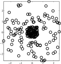
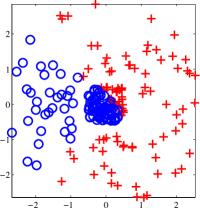
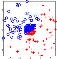
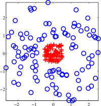
(a)

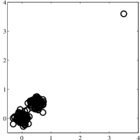
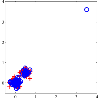
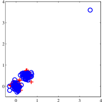
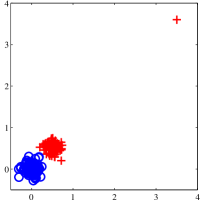
(b)

Original data

NCut

RatioCut

SDCut-QN

(c)

Figure 1: Results for $2$-demensional points bisection. The resulting two classes of points are shown in red ‘+’ and blue ‘$\circ$’ respectively. SDCut-QN succeeds in clustering the points as desired, while both RatioCut and NCut failed in these two cases.

To show that the proposed SDP methods have better solution quality than spectral methods we compare the graph-bisection results of RatioCut [76], Normalized Cut (NCut) [19] and SDCut-QN on two artificial 2-dimensional datasets.

As shown in Fig. 1, the first data set (the first row) contains two sets of points with different densities, and the second set contains an outlier. RatioCut and NCut fail to offer satisfactory results on both of the data sets, possibly due to the poor approximation of spectral relaxation. In contrast, our SDCut-QN achieves desired results on these data sets.

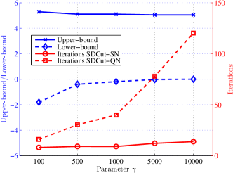
Figure 2: Results for graph bisection with different values of the parameter $\gamma$. The illustrated results are averaged over $10$ random graphs. Upper-bounds and lower-bounds achieved by SDCut-QN are shown in this figure (those of SDCut-SN is very similar and thus omitted). The relaxation becomes tighter (that is, upper-bounds and lower-bounds are closer) for larger $\gamma$. The number of iterations for both SDCut-SN and SDCut-QN grows with the increase of $\gamma$.

Secondly, to demonstrate the impact of the parameter $\gamma$, we test SDCut-QN and SDCut-SN on a random graph with $\gamma$ ranging from $10^{2}$ to $10^{4}$ ($\mathbf{A}$ and $\mathbf{B}_{i}$ in (1) are scaled such that $\lVert\mathbf{A}\rVert_{F}^{2}=\lVert\mathbf{B}\rVert_{F}^{2}=1$). The graph is generated with $1000$ vertices and all possible edges are assigned a non-zero weight uniformly sampled from $(0,1]$. As the resulting affinity matrices are dense, the DSYEVR routine in LAPACK package is used for eigen-decomposition. In Fig. 2, we show the upper-bounds, lower-bounds, number of iterations and time achieved by SDCut-QN and SDCut-SN, with respect to different values of $\gamma$. There are several observations: $i$) With the increase of $\gamma$, upper-bounds become smaller and lower-bounds become larger, which implies a tighter relaxation. $ii$) Both SDCut-QN and SDCut-SN take more iterations to converge when $\gamma$ is larger. $iii$) SDCut-SN uses fewer iterations than SDCut-QN. The above observations coincide with the analysis in Section 4.5. Using a larger parameter $\gamma$ yields better solution quality, but at the cost of slower convergence speed. The choice of a good $\gamma$ is data dependant. To reduce the difficulty of the choice of $\gamma$, the matrices $\mathbf{A}$ and $\mathbf{B}_{i}$ of Equation (1) are scaled such that the Frobenius norm is $1$ in the following experiments.

Thirdly, experiments are performed to evaluate another two factors affecting the speed of our methods: the sparsity of the affinity matrix $\mathbf{W}$ and the matrix size $n$. The numerical results corresponding to dense and sparse affinity matrices are shown in Table III and Table IV respectively. The sparse affinity matrices are generated from random graphs with $8$-neighbour connection. In these experiments, the size of matrix $\mathbf{W}$ is varied from $200$ to $5000$. ARPACK is used by SDCut-QN for partial eigen-decomposition of sparse problems, and DSYEVR is used for other cases. For both SDCut-QN and SDCut-SN, the number of iterations does not grow significantly with the increase of $n$. However, the running time is still correlated with $n$, since an eigen-decompostion of an $n\times n$ matrix needs to be computed at each iteration for both of our methods. We also find that the second-order method SDCut-SN uses significantly fewer iterations than the first-order method SDCut-QN. For dense affinity matrices, SDCut-SN runs consistently faster than SDCut-QN. In contrast for sparse affinity matrices, SDCut-SN is only faster than SDCut-QN on problems of size up to $n\geq 2000$. That is because the Lanczos method used by SDCut-QN (for partial eigen-decompostion) scales much better for large sparse matrices than the standard factorization method (DSYEVR) used by SDCut-SN (for full eigen-decomposition). The upper-/lower-bounds yielded by our methods are similar to those of the interior-point methods. Meanwhile, NCut and RatioCut run much faster than other methods, but offer significantly worse upper-bounds.

Finally, we evaluate SDCut-QN on a large dense graph with $10000$ nodes. The speed performance is compared on a single CPU core (using DSYEVR function of LAPACK as eigensolver) and a hybrid CPU+GPU workstation (using the DSYEVDX$\_2$STAGE function of MAGMA as eigensolver). The results are shown in Table V and we can see that the parallelization brings a $10$-fold speedup over running on a single CPU core. The lower-/upper-bounds are almost identical as there is no difference apart from the implementation of eigen-decompostion.

$n$, $m$	Methods	SDCut-QN	SDCut-SN	SeDuMi	SDPT3	MOSEK	NCut	RatioCut
$200$, $201$
	Time/Iters	$0.7$s/$67.7$	$\mathbf{0.6}\bf{s}$/$\mathbf{11.0}$	$10.4$s	$7.0$s	$5.5$s	$0.2$s	$0.2$s
	Upper-bound	$1.03$	$1.04$	$1.04$	$1.03$	$1.04$	$1.82$	$4.61$
	Lower-bound	$-0.63$	$-0.63$	$-0.58$	$-0.58$	$-0.58$	$-$	$-$
$500$, $501$
	Time/Iters	$1.9$s/$43.2$	$\mathbf{1.8}\bf{s}$/$\mathbf{9.7}$	$01$m$21$s	$33.9$s	$36.0$s	$0.3$s	$0.4$s
	Upper-bound	$2.94$	$2.96$	$2.93$	$2.92$	$2.93$	$4.01$	$9.23$
	Lower-bound	$-0.31$	$-0.31$	$-0.20$	$-0.20$	$-0.20$	$-$	$-$
$1000$, $1001$
	Time/Iters	$22.6$s/$39.9$	$\mathbf{13.0}\bf{s}$/$\mathbf{9.0}$	$08$m$21$s	$\dagger$	$02$m$36$s	$0.5$s	$0.9$s
	Upper-bound	$5.06$	$5.10$	$5.07$	$\dagger$	$5.04$	$6.10$	$13.28$
	Lower-bound	$-0.19$	$-0.19$	$0.02$	$\dagger$	$0.02$	$-$	$-$
$2000$, $2001$
	Time/Iters	$01$m$54$s/$34.9$	$\mathbf{54.3}\bf{s}$/$\mathbf{9.0}$	$55$m$45$s	$\dagger$	$22$m$25$s	$2.1$s	$2.9$s
	Upper-bound	$8.02$	$7.99$	$7.94$	$\dagger$	$7.95$	$9.00$	$20.85$
	Lower-bound	$-0.18$	$-0.18$	$0.21$	$\dagger$	$0.21$	$-$	$-$
$5000$, $5001$
	Time/Iters	$20$m$39$s/$27.1$	$\mathbf{11}$m$\mathbf{05}$s/$\mathbf{8.1}$	$14$h$55$m	$\dagger$	$04$h$40$m	$24.2$s	$15.4$s
	Upper-bound	$13.89$	$13.87$	$13.78$	$\dagger$	$15.60$	$14.91$	$33.46$
	Lower-bound	$-0.32$	$-0.32$	$0.51$	$\dagger$	$2.66$	$-$	$-$

TABLE III: Numerical results for graph bisection with dense affinity matrices. All the results are the average over $10$ random graphs. SDP based methods (the left five columns) achieve better upper-bounds than spectral methods (NCut and RatioCut). SDCut-SN uses fewer iterations than SDCut-QN and achieves the fastest speed of the five SDP based methods. $\dagger$  denotes the cases where SDPT3 fails to output feasible solutions.

$n$, $m$	Methods	SDCut-QN	SDCut-SN	SeDuMi	SDPT3	MOSEK	NCut	RatioCut
$200$, $201$
	Time/Iters	$6.0$s/$76.5$	$\mathbf{0.6}\bf{s}$/$\mathbf{11.0}$	$9.8$s	$7.3$s	$3.5$s	$0.1$s	$0.1$s
	Upper-bound	$-0.57$	$-0.57$	$-0.57$	$-0.57$	$-0.57$	$8.38$	$-0.48$
	Lower-bound	$-1.32$	$-1.32$	$-1.28$	$-1.28$	$-1.28$	$-$	$-$
$500$, $501$
	Time/Iters	$12.3$s/$65.3$	$\mathbf{3.1}\bf{s}$/$\mathbf{11.0}$	$01$m$36$s	$54.0$s	$40.5$s	$0.1$s	$0.2$s
	Upper-bound	$0.65$	$0.64$	$0.65$	$0.64$	$0.64$	$19.20$	$0.73$
	Lower-bound	$-0.41$	$-0.41$	$-0.30$	$-0.30$	$-0.30$	$-$	$-$
$1000$, $1001$
	Time/Iters	$28.5$s/$73.3$	$\mathbf{24.0}\bf{s}$/$\mathbf{11.8}$	$11$m$36$s	$\dagger$	$02$m$43$s	$0.1$s	$0.3$s
	Upper-bound	$1.35$	$1.35$	$1.35$	$\dagger$	$1.34$	$28.32$	$1.41$
	Lower-bound	$0.25$	$0.25$	$0.46$	$\dagger$	$0.46$	$-$	$-$
$2000$, $2001$
	Time/Iters	$\mathbf{01}$m$\mathbf{12}$s/$72.5$	$02$m$38$s/$\mathbf{12.5}$	$42$m$19$s	$\dagger$	$23$m$12$s	$0.3$s	$0.5$s
	Upper-bound	$2.43$	$2.43$	$2.41$	$\dagger$	$2.41$	$41.18$	$2.51$
	Lower-bound	$1.01$	$1.01$	$1.40$	$\dagger$	$1.40$	$-$	$-$
$5000$, $5001$
	Time/Iters	$\mathbf{04}$m$\mathbf{43}$s/$90.3$	$26$m$19$s/$\mathbf{13.2}$	$15$h$48$m	$\dagger$	$05$h$18$m	$1.2$s	$0.9$s
	Upper-bound	$4.00$	$3.99$	$3.95$	$\dagger$	$3.95$	$64.98$	$4.02$
	Lower-bound	$2.24$	$2.24$	$3.12$	$\dagger$	$3.12$	$-$	$-$

TABLE IV: Numerical results for graph bisection with sparse affinity matrices. All the results are the average over $10$ random graphs. The upper-bounds achieved by SDP based methods are close to each other and significantly better than spectral methods (NCut and RatioCut). The number of iterations for SDCut-SN is much less than SDCut-QN. For problems with $n\leq 1000$, SDCut-SN is faster than SDCut-QN. While for larger problems ($n\geq 2000$), SDCut-QN achieves faster speeds than SDCut-SN. $\dagger$  denotes the cases where SDPT3 fails to output feasible solutions.

	CPU	CPU+GPU
Time/Iters	$3$h$8$m/$24.0$	${18}{m}$/$24.0$
Upper-bound	$20.42$	$20.36$
Lower-bound	$-4.15$	$-4.15$

TABLE V: Graph bisection on large dense graphs ($n=10000,m=10001$). SDCut-QN is tested on $1$ core of Intel Xeon E$5$-$2680$ $2.7$GHz CPU ($20$MB cache) and a workstation with $1$ Intel Xeon E$5$-$2670$ $2.30$GHz CPU ($8$ cores and $20$MB cache) and $1$ NVIDIA Tesla K$40$c GPU. A $10$-fold speedup is achieved by using CPU+GPU compared with using CPU only.

5.2 Constrained Image Segmentation

We consider image segmentation with two types of quadratic constraints (with respect to $\mathbf{x}$): partial grouping constraints [20] and histogram constraints [77]. The affinity matrix $\mathbf{W}$ is sparse, so ARPACK is used by SDCut-QN for eigen-decomposition.

Besides interior-point SDP methods, we also compare our methods with graph-cuts [7, 8, 9] and two constrained spectral clustering method proposed by Maji et al. [78] (referred to as BNCut) and Wang and Davidson [79] (referred to as SMQC). BNCut and SMQC can encode only one quadratic constraint, but it is difficult (if not impossible) to generalize them to multiple quadratic constraints.

Partial Grouping Constraints The corresponding BQP formulation is Equation (24) in Table II. A feasible solution $\mathbf{x}$ to (24) can obtained from any random sample $\mathbf{z}$ as follows:

$$x_{i}=\left\{\begin{array}[]{ll}\mathrm{sign}(z_{i}-\theta_{f})&\mbox{if }(\mathbf{s}_{f})_{i}>0,\\ \mathrm{sign}(z_{i}-\theta_{b})&\mbox{if }(\mathbf{s}_{b})_{i}>0,\\ \mathrm{sign}(z_{i})&\mbox{otherwise},\end{array}\right.$$ (33)

where $\theta_{f}$ and $\theta_{b}$ are chosen from $[\min(\{z_{i}|(\mathbf{s}_{f})_{i}>0\}),+\infty)$ and $(-\infty,\max(\{z_{i}|(\mathbf{s}_{b})_{i}>0\}]$ respectively. Note that for any sample $\mathbf{z}$, $\mathbf{x}$ is feasible if $\theta_{f}=\min(\{z_{i}|(\mathbf{s}_{f})_{i}>0\})$ and $\theta_{b}=\max(\{z_{i}|(\mathbf{s}_{b})_{i}>0\})$.

Fig. 3 illustrates the result for image segmentation with partial grouping constraints on the Berkeley dataset [80]. All the test images are over-segmented into about $760$ superpixels. We find that BNCut did not accurately segment foreground, as it only incorporates a single set of grouping pixels (foreground). In contrast, our methods are able to accommodate multiple sets of grouping pixels and segment the foreground more accurately. In Table VI, we compare the CPU time and the upper-bounds of SDCut-QN, SeDuMi and SDPT3. SDCut-QN achieves objective values similar to that of SeDuMi and SDPT3, yet is over $10$ times faster.

Images

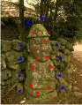
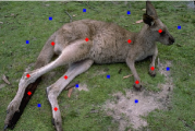
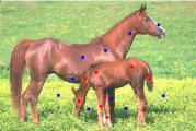
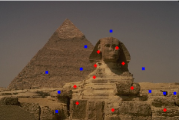
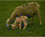
(a)

BNCut

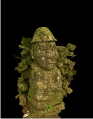
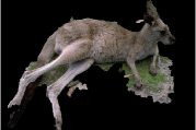
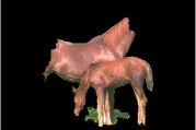
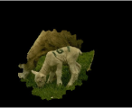
(b)

SDCut-QN

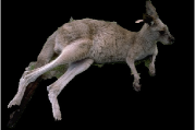
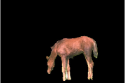
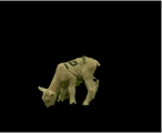
(c)

Figure 3: Image segmentation with partial grouping constraints. The top row shows the original images with $10$ labelled foreground (red markers) and $10$ background (blue markers) pixels. SDCut-QN achieves significantly better results than BNCut. The results of SeDuMi and SDPT3 are omitted, as they are similar to those of SDCut-QN.

Methods	SDCut-QN	SeDuMi	SDPT3
Time	$23.7$s	$6$m$12$s	$5$m$29$s
Upper-bound	$-116.10$	$-116.30$	$-116.32$

TABLE VI: Numerical results for image segmentation with partial grouping constraints. Time and upper-bound are the means over the five images in Fig. 3. SDCut-QN runs $10$ times faster than SeDuMi and SDPT3, and offers a similar upper-bound.

Images

(a)

GT

(b)

Graph cuts

unary

(c)

Graph cuts

(d)

SMQC

(e)

SDCut-QN

(f)

Figure 4: Image segmentation with histogram constraints (coarse over-segmentation). The number of superpixels is around $726$. From top to bottom are: original images, ground-truth (GT), superpixels, unary terms for graph-cuts, results of graph-cuts, SMQC and SDCut-QN. Results for other SDP based methods are similar to that of SDCut-QN and thus omitted. Graph cuts tends to mix together the foreground and background with similar color. SDCut-QN achieves the best segmentation results.

Methods	SDCut-QN	SDCut-SN	SeDuMi	SDPT3	MOSEK	GC	SMQC
Time/Iters	$32.3$s/$248.3$	$\mathbf{14.8}$s/$\mathbf{22.9}$	$2$m$57$s	$1$m$2$s	$1$m$19$s	$0.2$s	$5.1$s
F-measure	$0.930$	$0.925$	$0.928$	$0.926$	$0.928$	$0.722$	$0.832$
Upper-bound	$-120.0$	$-120.1$	$-120.1$	$-119.8$	$-120.1$	$-$	$-$
Lower-bound	$-126.8$	$-126.8$	$-126.7$	$-126.7$	$-126.7$	$-$	$-$

TABLE VII: Image segmentation with histogram constraints. Results are the average of the eight images shown in Fig. 4. SDCut-SN uses fewer iterations than SDCut-QN and is faster than all other SDP based methods. Graph cuts and SMQC exhibit worse F-measure scores than SDP based methods.

Histogram Constraints Given a random sample $\mathbf{z}$, a feasible solution $\mathbf{x}$ to the corresponding BQP formulation (25) can be obtained through $\mathbf{x}=\mathrm{sign}(\mathbf{z}-\theta)$, where

$$\theta\!=\!\left\{\begin{array}[]{ll}\!0\!&\mbox{if }\lvert\mathbf{1}^{\!\top}\mathrm{sign}(\mathbf{z})\rvert\!\leq\!\kappa n,\\ \!(\tilde{z}_{\lfloor\frac{n+\kappa\!n\!}{2}\rfloor}\!+\!\tilde{z}_{\lfloor\frac{n+\kappa\!n\!}{2}\rfloor+\!1})/2\!&\mbox{if }{\mathbf{1}^{\!\top}\mathrm{sign}(\mathbf{z})\!>\!\kappa n},\\ \!(\tilde{z}_{\lceil\frac{n-\kappa\!n\!}{2}\rceil}\!+\!\tilde{z}_{\lceil\frac{n-\kappa\!n\!}{2}\rceil+\!1})/2\!&\mbox{if }{\mathbf{1}^{\!\top}\mathrm{sign}(\mathbf{z})\!<\!-\kappa n},\end{array}\right.$$ (37)

and $\tilde{\mathbf{z}}$ is obtained by sorting $\mathbf{z}$ in descending order. For graph cuts methods, the histogram constraint is encoded as unary terms: $\varphi_{i}=-\ln\big{(}\mathrm{Pr}(\mathbf{f}_{i}|\mbox{fore})/\mathrm{Pr}(\mathbf{f}_{i}|\mbox{back})\big{)}$, $i=1,2,\dots,n$. $\mathrm{Pr}(\mathbf{f}_{i}|\mbox{fore})$ and $\mathrm{Pr}(\mathbf{f}_{i}|\mbox{back})$ are probabilities for the color of the $i$th pixel belonging to foreground and background respectively.

Fig. 4 and Table VII demonstrate the results for image segmentation with histogram constraints. We can see that unary terms (the second row in Fig. 4) are not ideal especially when the color distribution of foreground and background are overlapped. For example in the first image, the white collar of the person in the foreground have similar unary terms with the white wall in the background. The fourth row of Fig. 4 shows that the unsatisfactory unary terms degrade the segmentation results of graph cuts methods significantly.

The average F-measure of all evaluated methods are reported in Table VII. Our methods outperforms graph cuts and SMQC in terms of F-measure. As for the running time, SDCut-SN is faster than all other SDP-based methods (that is, SDCut-QN, SeDuMi, SDPT3 and MOSEK). As expected, SDCut-SN uses much less ($1/6$) iterations than SDCut-QN. SDCut-QN and SDCut-SN have comparable upper-bounds and lower-bounds than interior-point methods.

From Table VII, we can find that SMQC is faster than our methods. However, SMQC does not scale well to large problems since it needs to compute full eigen-decomposition. We also test SDCut-QN and SMQC on problems with a larger number of superpixels ($9801$). Both of the algorithms achieve similar segmentation results, but SDCut-QN is much faster than SMQC ($23$m$21$s vs. $4$h$9$m).

5.3 Image Co-segmentation

Images

(a)

LowRank

(b)

SDCut-QN

(c)

Images

(d)

LowRank

(e)

SDCut-QN

(f)

Figure 5: Image co-segmentation on Weizman horses and MSRC datasets. The original images, the results (score vectors) of LowRank and SDCut-QN are illustrated from top to bottom. Other methods produce similar segmentation results.

The task of image co-segmentation [38] aims to partition a common object from multiple images simultaneously. In this work, the Weizman horses and MSRC datasets are tested. There are $6\!\thicksim\!10$ images in each of four classes, namely “car-front”, “car-back”, “face” and “horse”. Each image is oversegmented to $400\!\thicksim\!700$ superpixels. The number of binary variables $n$ is then increased to $4000\!\thicksim\!7000$.

The BQP formulation for image co-segmentation can be found in Table II (see [38] for details). The matrix $\mathbf{A}$ can be decomposed into a sparse matrix and a structural matrix, such that ARPACK can be used by SDCut-QN. Each vector $\mathbf{z}=[{\mathbf{z}^{(1)}}^{\!\top},\cdots,{\mathbf{z}^{(K)}}^{\!\top}]^{\!\top}$ (where $\mathbf{z}^{i}$ corresponds to the $i$-th image) randomly sampled from $\mathcal{N}(\mathbf{0},\mathbf{X}^{\star})$ is discretized to a feasible BQP solution as follows:

$$\mathbf{x}=\left[\mathrm{sign}(\mathbf{z}^{(1)}-\theta^{(1)})^{\!\top},\cdots,\mathrm{sign}(\mathbf{z}^{(K)}-\theta^{(K)})^{\!\top}\right]^{\!\top},$$ (38)

where $\theta^{(i)}$ can be obtained as (37).

We compare our methods with the low-rank factorization method [38] (referred to as LowRank) and interior-point methods. As we can see in Table VIII, SDCut-QN takes $10$ times more iterations than SDCut-SN, but still runs faster than SDCut-SN especially when the size of problem is large (see “face” data). The reason is that SDCut-QN can exploit the specific structure of matrix $\mathbf{A}$ in eigen-decomposition. SDCut-QN runs also $5$ times faster than LowRank. All methods provide similar upper-bounds (primal objective values), and the score vectors shown in Fig. 5 also show that the evaluated methods achieve similar visual results.

Data, $n$, $m$	Methods	SDCut-QN	SDCut-SN	SeDuMi	MOSEK	LowRank
car-back, $4012$, $4018$	Time/Iters	$\mathbf{06}$m$\mathbf{08}$s/$140$	$09$m$59$s/$\mathbf{15}$	$07$h$02$m	$02$h$54$m	$28$m$44$s
	Upper-bound	$12.71$	$12.71$	$12.74$	$12.74$	$12.64$
	Lower-bound	$-7.41$	$-7.41$	$-7.30$	$-7.30$	$-$
car-front, $4017$, $4023$
	Time/Iters	$\mathbf{07}$m$\mathbf{32}$s/$188$	$11$m$25$s/$\mathbf{16}$	$07$h$04$m	$02$h$54$m	$59$m$47$s
	Upper-bound	$8.16$	$8.16$	$8.16$	$8.16$	$8.61$
	Lower-bound	$-7.67$	$-7.67$	$-7.56$	$-7.56$	$-$
face, $6684$, $6694$
	Time/Iters	$\mathbf{08}$m$\mathbf{18}$s/$164$	$43$m$57$s/$\mathbf{16}$	$>24$hrs	$12$h$06$m	$40$m$56$s
	Upper-bound	$12.65$	$12.65$	$-$	$12.96$	$20.53$
	Lower-bound	$-9.73$	$-9.73$	$-$	$-9.53$	$-$
horse, $4587$, $4597$
	Time/Iters	$\mathbf{06}$m$\mathbf{15}$s/$167$	$17$m$01$s/$\mathbf{16}$	$11$h$03$m	$04$h$14$m	$42$m$14$s
	Upper-bound	$14.78$	$14.78$	$14.76$	$14.76$	$15.77$
	Lower-bound	$-6.83$	$-6.83$	$-6.69$	$-6.69$	$-$

TABLE VIII: Numerical results for image co-segmentation. All the evaluated are SDP based methods and achieve similar upper-bounds and lower-bounds. SDCut-QN runs significantly faster than other methods, although it needs more iterations to converge than SDCut-SN.

5.4 Graph Matching

In the graph matching problems considered in this work, each of the $K$ source points must be matched to one of the $L$ target points, where $L\geq K$. The optimal matching should maximize both of the local feature similarities between matched-pairs and the structure similarity between the source and target graphs.

The BQP formulation of graph matching can be found in Table II, which can be relaxed to:

$$\min_{\mathbf{x},\mathbf{X}} \quad\langle\mathbf{X},\mathbf{H}\rangle+\mathbf{h}^{\!\top}\mathbf{x}$$ (39a)

$$\mathrm{s.t.} \quad\mathrm{diag}(\mathbf{X})=\mathbf{x},$$ (39b)

$$\quad\textstyle{\sum_{j=1}^{L}}x_{(i-1)L+j}=1,\,\forall i\in\mathcal{K},$$ (39c)

$$\quad X_{\scriptsize(i-1)L+j,(i-1)L+k}=0,\forall i\in\mathcal{K},\,\,j\neq k\in\mathcal{L},$$ (39d)

$$\quad X_{(j-1)L+i,(k-1)L+i}=0,\forall i\in\mathcal{L},\,\,j\neq k\in\mathcal{K},$$ (39e)

$$\quad{\scriptsize\begin{bmatrix}1&\mathbf{x}^{\!\top}\\ \mathbf{x}&\mathbf{X}\end{bmatrix}}\in\mathcal{S}^{KL+1},$$ (39f)

where $\mathcal{K}=\{1,\cdots,K\}$ and $\mathcal{L}=\{1,\cdots,L\}$.

A feasible binary solution $\mathbf{x}$ is obtained by solving the following linear program (see [37] for details):

$$\max_{\mathbf{x}\geq\mathbf{0}}\quad \mathbf{x}^{{\!\top}}\mathrm{diag}(\mathbf{X}^{\star}),$$ (40a)

$$\ \ \mathrm{s.t.}\quad \ \textstyle{\sum_{j=1}^{L}}\mathbf{x}_{\tiny(i-1)\!L+j}=1,\forall i\in\mathcal{K},$$ (40b)

$$\ \textstyle{\sum_{i=1}^{K}}\mathbf{x}_{\tiny(i-1)\!L+j}\leq 1,\forall j\in\mathcal{L}.$$ (40c)

Two-dimensional points are randomly generated for evaluation. Table IX shows the results for different problem sizes: $n$ ranges from $201$ to $3201$ and $m$ ranges from $3011$ to $192041$. SDCut-SN and SDCut-QN achieves exactly the same upper-bounds as interior-point methods and comparable lower-bounds. Regarding the running time, SDCut-SN takes much less number of iterations to converge and is relatively faster (within $2$ times) than SDCut-QN. Our methods run significantly faster than interior-point methods. Taking the case $K\times L=25\times 50$ as an example, SDCut-SN and SDCut-QN converge at around $4$ minutes and interior-point methods do not converge within $24$ hours. Furthermore, interior-point methods runs out of $100$G memory limit when the number of primal constraints $m$ is over $10^{5}$. SMAC [22], a spectral method incorporating affine constrains, is also evaluated in this experiment, which provides worse upper-bounds and error ratios.

$K\!\times\!L$, $n$, $m$	Methods	SDCut-QN	SDCut-SN	SeDuMi	SDPT3	MOSEK	SMAC
$10\times 20$, $201$, $3011$
	Time/Iters	$5.8$s/$262.6$	$\mathbf{1.7}\bf{s}$/$\mathbf{34.2}$	$02$m$17$s	$45.0$s	$30.7$s	$0.1$s
	Error ratio	$1/100$	$1/100$	$1/100$	$1/100$	$1/100$	$1/100$
	Upper-bound	$-1.30\!\times\!10^{-1}$	$-1.30\!\times\!10^{-1}$	$-1.30\!\times\!10^{-1}$	$-1.30\!\times\!10^{-1}$	$-1.30\!\times\!10^{-1}$	$-1.27\!\times\!10^{-1}$
	Lower-bound	$-1.31\!\times\!10^{-1}$	$-1.31\!\times\!10^{-1}$	$-1.31\!\times\!10^{-1}$	$-1.30\!\times\!10^{-1}$	$-1.30\!\times\!10^{-1}$	$-$
$15\times 30$, $451$, $10141$
	Time/Iters	$22.5$s/$359.7$	$\mathbf{11.2}\bf{s}$/$\mathbf{35.7}$	$01$h$34$m	$15$m$48$s	$30$m$38$s	$0.3$s
	Error ratio	$1/150$	$1/150$	$1/150$	$1/150$	$1/150$	$6/150$
	Upper-bound	$-3.77\!\times\!10^{-2}$	$-3.77\!\times\!10^{-2}$	$-3.77\!\times\!10^{-2}$	$-3.77\!\times\!10^{-2}$	$-3.77\!\times\!10^{-2}$	$-2.01\!\times\!10^{-2}$
	Lower-bound	$-3.81\!\times\!10^{-2}$	$-3.81\!\times\!10^{-2}$	$-3.78\!\times\!10^{-2}$	$-3.79\!\times\!10^{-2}$	$-3.78\!\times\!10^{-2}$	$-$
$20\times 40$, $801$, $24021$
	Time/Iters	$01$m$27$s/$405.2$	$\mathbf{51.2}\bf{s}$/$\mathbf{41.7}$	$17$h$48$m	$02$h$09$m	$04$h$39$m	$0.2$s
	Error ratio	$1/200$	$1/200$	$1/200$	$1/200$	$1/200$	$6/200$
	Upper-bound	$4.01\!\times\!10^{-2}$	$4.01\!\times\!10^{-2}$	$4.01\!\times\!10^{-2}$	$4.01\!\times\!10^{-2}$	$4.01\!\times\!10^{-2}$	$4.29\!\times\!10^{-2}$
	Lower-bound	$3.93\!\times\!10^{-2}$	$3.93\!\times\!10^{-2}$	$3.99\!\times\!10^{-2}$	$3.98\!\times\!10^{-2}$	$3.99\!\times\!10^{-2}$	$-$
$25\times 50$, $1251$, $46901$
	Time/Iters	$04$m$05$s/$384.0$	$\mathbf{03}$m$\mathbf{50}$s/$\mathbf{41.0}$	$>24$hrs	$>24$hrs	$>24$hrs	$0.3$s
	Error ratio	$0/250$	$0/250$	$-$	$-$	$-$	$3/250$
	Upper-bound	$1.04\!\times\!10^{-1}$	$1.04\!\times\!10^{-1}$	$-$	$-$	$-$	$1.06\!\times\!10^{-1}$
	Lower-bound	$1.03\!\times\!10^{-1}$	$1.03\!\times\!10^{-1}$	$-$	$-$	$-$	$-$
$30\times 60$, $1801$, $81031$
	Time/Iters	$14$m$43$s/$500.0$	$\mathbf{10}$m$\mathbf{20}$s/$\mathbf{50.0}$	$>24$hrs	$>24$hrs	$>24$hrs	$0.4$s
	Error ratio	$2/300$	$2/300$	$-$	$-$	$-$	$4/300$
	Upper-bound	$1.59\!\times\!10^{-1}$	$1.59\!\times\!10^{-1}$	$-$	$-$	$-$	$1.60\!\times\!10^{-1}$
	Lower-bound	$1.58\!\times\!10^{-1}$	$1.58\!\times\!10^{-1}$	$-$	$-$	$-$	$-$
$40\times 80$, $3201$, $192041$
	Time/Iters	$03$h$02$m/$500.0$	$\mathbf{02}$h$\mathbf{26}$m/$\mathbf{50.0}$	Out of mem.	Out of mem.	Out of mem.	$1.2$s
	Error ratio	$1/400$	$1/400$	$-$	$-$	$-$	$9/400$
	Upper-bound	$2.63\!\times\!10^{-1}$	$2.63\!\times\!10^{-1}$	$-$	$-$	$-$	$2.66\!\times\!10^{-1}$
	Lower-bound	$2.61\!\times\!10^{-1}$	$2.61\!\times\!10^{-1}$	$-$	$-$	$-$	$-$

TABLE IX: Numerical results for graph matching, which are the mean over $10$ random graphs. For the fourth and fifth models, interior-point methods including Sedumi, SDPT3 and Mosek do not converge within $24$ hours. For the last model with around $2\times 10^{5}$ constraints, Sedumi, SDPT3 and Mosek run out of $100$G memory limit. SDCut-SN uses fewer iterations than SDCut-QN and achieves the fastest speed over all SDP based methods. All SDP based methods achieve the same upper-bounds and error rates. The lower-bounds for SDCut-SN and SDCut-QN are slightly worse than interior-point methods. SMAC provides worse upper-bounds and error rates than SDP-based methods.

5.5 Image Deconvolution

Methods	SDCut-SN	SeDuMi	MOSEK	TRWS	MPLP
Time/Iters	$\mathbf{2}$m$\mathbf{27}$s/$\mathbf{20.5}$	$2$h$48$m	$21$m$33$s	$20$m	$20$m
Error	$0.091$	$\mathbf{0.074}$	$0.083$	$0.111$	$0.112$
Upper-bound	$-988.3$	$\mathbf{-988.8}$	$-988.8$	$-986.9$	$-987.4$
Lower-bound	$-1054.2$	$\mathbf{-993.7}$	$-993.7$	$-1237.9$	$-1463.8$

TABLE X: Image deconvolution ($n=2250$, $m=2250$). The results are the average over two models in Figure 6. TRWS and MPLP are stopped at $20$ minutes. Compared to TRWS and MPLP, SDCut-SN achieves better upper-/lower-bounds and uses less time. The bounds given by SDCut-SN is comparable to those of interior-point methods.

Image deconvolution with a known blurring kernel is typically equivalent to solving a regularized linear inverse problem (see (28) in Table II). In this experiment, we test our algorithms on two binary $30\times 75$ images blurred by an $11\times 11$ Gaussian kernel. LP based methods such as TRWS [12] and MPLP [13] are also evaluated. Note that the resulting models are difficult for graph cuts or LP relaxation based methods in that it is densely connected and contains a large portion of non-submodular pairwise potentials. We can see from Fig. 6 and Table X that QPBO [7, 8, 9] leaves most of pixels unlabelled and LP methods (TRWS and MPLP) achieves worse segmentation accuracy. SDCut-SN achieves a $10$-fold speedup over interior-point methods while keep comparable upper-/lower-bounds. Using much less runtime, SDCut-SN still yields significantly better upper-/lower-bounds than LP methods.

Images

Blurred Images

SDCut-SN

MOSEK

QPBO

TRWS

MPLP

Figure 6: Image deconvolution. QPBO cannot label most of pixels (grey pixels denote unlabelled pixels), as the MRF models are highly non-submodular. SDCut-SN and MOSEK have similar segmentation results. TRWS and MPLP achieve worse segmentation results than our methods.

5.6 Chinese Character Inpainting

The MRF models for Chinese character inpainting are obtained from the OpenGM benchmark [82], in which the unary terms and pairwise terms are learned using decision tree fields [75]. As there are non-submodular terms in these models, they cannot be solved exactly using graph cuts. In this experiments, all models are firstly reduced using QPBO and different algorithms are compared on the $100$ reduced models. Our approach is compared to LP-based methods, including TRWS, MPLP. From the results shown in Table XI, we can see that SDCut-SN runs much faster than interior-point methods (SeDuMi and MOSEK) and has similar upper-bounds and lower-bounds. SDCut-SN is also better than TRWS and MPLP in terms of upper-bound and lower-bound. An extension of MPLP (refer to as MPLP-C) [81, 14], which adds violated cycle constraints iteratively, is also evaluated in this experiment. In MPLP-C, $1000$ LP iterations are performed initially and then $20$ cycle constraints are added at every $20$ LP iteration. MPLP-C performs worse than SDCut-SN under the runtime limit of $5$ minutes, and outperforms SDCut-SN with a much longer runtime limit ($1$ hour). We also find that SDCut-SN achieves better lower-bounds than MPLP-C on the instances with more edges (pairwise potential terms). Note that the time complexity of MPLP-C (per LP iteration) is proportional to the number of edges, while the time complexity of SDCut-SN (see Table I) is less affected by the edge number. It should be also noticed that SDCut-SN uses much less runtime than MPLP-C, and its bound quality can be improved by adding linear constraints (including cycle constraints) as well [83].

Methods	SDCut-SN	SeDuMi	MOSEK	TRWS	MPLP	MPLP-C ($5$m)	MPLP-C ($1$hr)
Time/Iters	${22.7}$s/${18.4}$	$3$m$50$s	$42$s	${23.5}$s	$24.9$s	$5$m	$51$m$24$s
Upper-bound	$-49525.5$	${-49525.5}(31)$	$-49525.5(30)$	$-49511.9(79)$	$-49403.4(100)$	$-49410.4(85)$	$-49495.8(47)$
Lower-bound	$-49683.0$	${-49676.2}(0)$	$-49676.2(0)$	$-50119.4(100)$	$-50119.4(100)$	$-49908.7(72)$	$-49614.0(7)$

TABLE XI: Chinese character inpainting using decision tree fields ($n=191\sim 1522$, $m=191\sim 1522$). The results are the average over $100$ models. The numbers of instances on which SDCut-SN performs better are shown in the parentheses. The upper-/lower-bounds given by SDCut-SN is comparable to those of interior-point methods. SDCut-SN also achieves better solutions than TRWS, MPLP and MPLP-C ($5$m). Using a much longer runtime ($55$m$24$s vs. $22.7$s), MPLP-C outperforms SDCut-SN.

6 Conclusion

In this paper, we have presented a regularized SDP algorithm (SDCut) for BQPs. SDCut produces bounds comparable to the conventional SDP relaxation, and can be solved much more efficiently. Two algorithms are proposed based on quasi-Newton methods (SDCut-QN) and smoothing Newton methods (SDCut-SN) respectively. Both SDCut-QN and SDCut-SN are more efficient than classic interior-point algorithms. To be specific, SDCut-SN is faster than SDCut-QN for small to medium sized problems. If the matrix to be eigen-decomposed, $\mathbf{C}(\mathbf{u})$, has a special structure (for example, sparse or low-rank) such that matrix-vector products can be computed efficiently, SDCut-QN is much more scalable to large problems. The proposed algorithms have been applied to several computer vision tasks, which demonstrate their flexibility in accommodating different types of constraints. Experiments also show the computational efficiency and good solution quality of SDCut. We have made the code available online.

Acknowledgements We thank the anonymous reviewers for the constructive comments on Propositions 1 and 4.

This work was in part supported by ARC Future Fellowship FT120100969. This work was also in part supported by the Data to Decisions Cooperative Research Centre.

7 Proofs

7.1 Proof of Proposition 1

Proof.

($i$) Let $t:=\frac{1}{2\gamma}$ and $\mathcal{P}:=\{\mathbf{X}\in\mathcal{S}^{n}_{+}|\langle\mathbf{B}_{i},\mathbf{X}\rangle=b_{i},i\in\mathcal{I}_{eq};\langle\mathbf{B}_{i},\mathbf{X}\rangle\leq b_{i},i\in\mathcal{I}_{in}\}$, we have

$$\lvert\mathrm{p}(\mathbf{X}^{\star})-\mathrm{p}(\mathbf{X}^{\star}_{\gamma})\rvert\leq \mathrm{p}(\mathbf{X}^{\star}_{\gamma})+\frac{1}{2\gamma}\lVert\mathbf{X}^{\star}_{\gamma}\rVert^{2}_{F}-\mathrm{p}(\mathbf{X}^{\star})$$ (41)

$$= \min_{\mathbf{X}\in\mathcal{P}}\mathrm{p}(\mathbf{X})+t\lVert\mathbf{X}\rVert^{2}_{F}-\mathrm{p}(\mathbf{X}^{\star}):=\theta(t).$$

As a pointwise minimum of affine functions of $t$, $\theta(t)$ is concave and continuous. It is also easy to find that $\theta(0)=0$ and $\theta(t)$ is monotonically increasing on $\mathbb{R}_{+}$. So for any $\epsilon>0$, there is a $t>0$ (and equivalently $\gamma=\frac{1}{2t}>0$) such that $\lvert\mathrm{p}(\mathbf{X}^{\star})-\mathrm{p}(\mathbf{X}^{\star}_{\gamma})\rvert<\epsilon$.

($ii$) By the definition of $\mathbf{X}^{\star}_{\gamma_{1}}$ and $\mathbf{X}^{\star}_{\gamma_{2}}$, it is clear that $\mathrm{p}_{\gamma_{1}}(\mathbf{X}_{\gamma_{1}}^{\star})\leq\mathrm{p}_{\gamma_{1}}(\mathbf{X}_{\gamma_{2}}^{\star})$ and $\mathrm{p}_{\gamma_{2}}(\mathbf{X}_{\gamma_{2}}^{\star})\leq\mathrm{p}_{\gamma_{2}}(\mathbf{X}_{\gamma_{1}}^{\star})$. Then we have $\mathrm{p}_{\gamma_{1}}(\mathbf{X}_{\gamma_{1}}^{\star})-\frac{\gamma_{2}}{\gamma_{1}}\mathrm{p}_{\gamma_{2}}(\mathbf{X}_{\gamma_{1}}^{\star})=(1\!-\!\frac{\gamma_{2}}{\gamma_{1}})\cdot\mathrm{p}(\mathbf{X}^{\star}_{\gamma_{1}})\leq\ \mathrm{p}_{\gamma_{1}}(\mathbf{X}_{\gamma_{2}}^{\star})-\frac{\gamma_{2}}{\gamma_{1}}\mathrm{p}_{\gamma_{2}}(\mathbf{X}_{\gamma_{2}}^{\star})=(1\!-\!\frac{\gamma_{2}}{\gamma_{1}})\cdot\mathrm{p}(\mathbf{X}^{\star}_{\gamma_{2}})$. Because $\gamma_{2}/\gamma_{1}>1$, $\mathrm{p}(\mathbf{X}^{\star}_{\gamma_{1}})\geq\mathrm{p}(\mathbf{X}^{\star}_{\gamma_{2}})$. ∎

7.2 Proof of Proposition 2

Proof.

The Lagrangian of the primal problem (5) is:

$$\mathrm{L}(\mathbf{X},\mathbf{u},\mathbf{Z})= \langle\mathbf{X},\mathbf{A}\rangle-\langle\mathbf{X},\mathbf{Z}\rangle+\frac{1}{2\gamma}\lVert\mathbf{X}\rVert_{F}^{2}$$

$$+\textstyle{\sum_{i=1}^{m}}u_{i}(\langle\mathbf{X},\mathbf{B}_{i}\rangle\!-\!b_{i}),$$ (42)

where $\mathbf{u}\in\mathbb{R}^{|\mathcal{I}_{eq}|}\times\mathbb{R}^{|\mathcal{I}_{in}|}_{+}$ and $\mathbf{Z}\in\mathcal{S}^{n}_{+}$ are Lagrangian multipliers.

Supposing (5) and (42) are feasible, strong duality holds and $\nabla_{\mathbf{X}}\mathrm{L}(\mathbf{X}^{\star},\mathbf{u}^{\star},\mathbf{Z}^{\star})=0$, where $\mathbf{X}^{\star}$, $\mathbf{u}^{\star}$ and $\mathbf{Z}^{\star}$ are optimal solutions. Then we have that

$$\mathbf{X}^{\star}\!=\!\gamma(\mathbf{Z}^{\star}\!-\!\mathbf{A}\!-\!\textstyle{\sum_{i=1}^{m}}u_{i}^{\star}\mathbf{B}_{i})=\gamma(\mathbf{Z}^{\star}\!+\!\mathbf{C}(\mathbf{u}^{\star})).$$ (43)

By substituting $\mathbf{X}^{\star}$ to (42), we have the dual:

$$\max_{\mathbf{u}\in\mathbb{R}^{|\mathcal{I}_{eq}|}\times\mathbb{R}^{|\mathcal{I}_{in}|}_{+},\,\mathbf{Z}\in\mathcal{S}^{n}_{+}} \,\,-\mathbf{u}^{{\!\top}}\mathbf{b}-\frac{\gamma}{2}\lVert\mathbf{Z}+\mathbf{C}(\mathbf{u})\rVert_{F}^{2}.$$ (44)

The variable $\mathbf{Z}$ can be further eliminated as follows. Given a fixed $\mathbf{u}$, (44) can be simplified to: $\min_{\mathbf{Z}\in\mathcal{S}^{n}_{+}}\ \lVert\mathbf{Z}+\mathbf{C}(\mathbf{u})\rVert_{F}^{2}$, which is proved to has the solution $\mathbf{Z}^{\star}=\Pi_{\mathcal{S}^{n}_{+}}(-\mathbf{C}(\mathbf{u}))$ (see [84] or Section 8.1.1 of [85]). Note that $\mathbf{C}(\mathbf{u})=\Pi_{\mathcal{S}^{n}_{+}}(\mathbf{C}(\mathbf{u}))-\Pi_{\mathcal{S}^{n}_{+}}(-\mathbf{C}(\mathbf{u}))$, so $\mathbf{Z}^{\star}+\mathbf{C}(\mathbf{u})=\Pi_{\mathcal{S}^{n}_{+}}(\mathbf{C}(\mathbf{u}))$. By substituting $\mathbf{Z}$ into (44) and (43), we have the simplified dual (6) and Equation (7). ∎

7.3 Proof of Proposition 3

Proof.

Set $\zeta(\mathbf{X}):=\frac{1}{2}\lVert\Pi_{\mathcal{S}^{n}_{+}}(\mathbf{X})\rVert_{F}^{2}=\frac{1}{2}\sum_{i=1}^{n}(\max(0,\lambda_{i}))^{2}$, where $\lambda_{i}$ denotes the $i$-th eigenvalue of $\mathbf{X}$. $\zeta(\mathbf{X})$ is a separable spectral function associated with the function $\mathrm{g}(x)=\frac{1}{2}(\max(0,x))^{2}$. $\zeta:\mathcal{S}^{n}\rightarrow\mathbb{R}$ is continuously differentiable but not necessarily twice differentiable at $\mathbf{X}\in\mathcal{S}^{n}$, as $\mathrm{g}:\mathbb{R}\rightarrow\mathbb{R}$ has the same smoothness property (see [86, 87, 88]). We also have $\nabla\zeta(\mathbf{X})=\Pi_{\mathcal{S}^{n}_{+}}(\mathbf{X})$. ∎

7.4 The Spherical Constraint

Before proving Proposition 4, we first give the following theorem.

Theorem 5.

(The spherical constraint). For any $\mathbf{X}\in\mathcal{S}^{n}_{+}$, we have the inequality $\lVert\mathbf{X}\rVert_{F}\leq\mathrm{trace}(\mathbf{X})$, in which the equality holds if and only if $\mathrm{rank}(\mathbf{X})=1$.

Proof.

The proof given here is an extension of the one in [89]. We have $\lVert\mathbf{X}\rVert_{F}^{2}=\mathrm{trace}(\mathbf{X}\mathbf{X}^{\!\top})=\sum_{i=1}^{n}\lambda^{2}_{i}\leq(\mathrm{trace}(\mathbf{X}))^{2}$, where $\lambda_{i}\geq 0$ denotes the $i$-th eigenvalue of $\mathbf{X}$. Note that $\lVert\mathbf{X}\rVert_{F}=\mathrm{trace}(\mathbf{X})$ (that is $\sum_{i=1}^{n}\lambda^{2}_{i}=(\sum_{i=1}^{n}\lambda_{i})^{2}$), if and only if there is only one non-zero eigenvalue of $\mathbf{X}$, that is, $\mathrm{rank}(\mathbf{X})=1$. ∎

7.5 Proof of Proposition 4

Proof.

Firstly, we have the following inequalities:

$$\mathrm{p}(\mathbf{X}^{\star})=\mathrm{p}_{\gamma}(\mathbf{X}^{\star})-\frac{\lVert\mathbf{X}^{\star}\rVert^{2}_{F}}{2\gamma}\geq\mathrm{p}_{\gamma}(\mathbf{X}^{\star})-\frac{(\mathrm{trace}(\mathbf{X}^{\star}))^{2}}{2\gamma},$$ (45)

where the second inequality is based on Theorem 5. For the BQP (3) that we consider, it is easy to see $\mathrm{trace}(\mathbf{X}^{\star})=n$. Furthermore, $\mathrm{p}_{\gamma}(\mathbf{X}^{\star})\geq\mathrm{p}_{\gamma}(\mathbf{X}^{\star}_{\gamma})$ holds by definition. Then we have that

$$\mathrm{p}(\mathbf{X}^{\star})\geq\mathrm{p}_{\gamma}(\mathbf{X}^{\star}_{\gamma})-\frac{n^{2}}{2\gamma}.$$ (46)

It is known that the optimum of the original SDP problem (4) is a lower-bound on the optimum of the BQP (3) (denoted by $p^{\star}$): $\mathrm{p}(\mathbf{X}^{\star})\leq p^{\star}$. Then according to (46), we have $\mathrm{p}_{\gamma}(\mathbf{X}^{\star}_{\gamma})-\frac{n^{2}}{2\gamma}\leq\mathrm{p}(\mathbf{X}^{\star})\leq p^{\star}$. Finally based on the strong duality, the primal objective value is not smaller than the dual objective value in the feasible set (see for example [85]): $\mathrm{d}_{\gamma}(\mathbf{u})\leq\mathrm{p}_{\gamma}(\mathbf{X}^{\star}_{\gamma})$, where $\mathbf{u}\in\mathbb{R}_{\vphantom{+}}^{|\mathcal{I}_{eq}|}\times\mathbb{R}_{+}^{|\mathcal{I}_{in}|}$, $\gamma>0$. In summary, we have: $\mathrm{d}_{\gamma}(\mathbf{u})-\frac{n^{2}}{2\gamma}\leq\mathrm{p}_{\gamma}(\mathbf{X}^{\star}_{\gamma})-\frac{n^{2}}{2\gamma}\leq\mathrm{p}(\mathbf{X}^{\star})\leq p^{\star},\,\forall\mathbf{u}\in\mathbb{R}_{\vphantom{+}}^{|\mathcal{I}_{eq}|}\times\mathbb{R}_{+}^{|\mathcal{I}_{in}|},\forall\gamma>0$. ∎

Peng Wang received the B.S. degree in electrical engineering and automation, and the PhD degree in control science and engineering from Beihang University, China, in 2004 and 2011, respectively. He is now a post-doctoral researcher at the University of Adelaide.

Chunhua Shen is a Professor at School of Computer Science, The University of Adelaide. His research interests are in the intersection of computer vision and statistical machine learning. He studied at Nanjing University, at Australian National University, and received his PhD degree from University of Adelaide. In 2012, he was awarded the Australian Research Council Future Fellowship.

Anton van den Hengel is a Professor and the Founding Director of the Australian Centre for Visual Technologies, at the University of Adelaide, focusing on innovation in the production and analysis of visual digital media. He received the Bachelor of mathematical science degree, Bachelor of laws degree, Master’s degree in computer science, and the PhD degree in computer vision from The University of Adelaide in 1991, 1993, 1994, and 2000, respectively.

Philip H. S. Torr received the Ph.D. (D.Phil.) degree from the Robotics Research Group at the University of Oxford, Oxford, U.K., under Prof. D. Murray of the Active Vision Group. He was a research fellow at Oxford for another three years. He left Oxford to work as a research scientist with Microsoft Research for six years, first with Redmond, WA, USA, and then with the Vision Technology Group, Cambridge, U.K., founding the vision side of the Machine Learning and Perception Group. Currently, he is a professor in computer vision and machine learning with Oxford University, Oxford, U.K.

Appendix

In this section, we present some computational details.

A.1 Preliminaries

A.1.1 Euclidean Projection onto the P.S.D. Cone

Theorem A.1.

The Euclidean projection of a symmetric matrix $\mathbf{X}\in\mathcal{S}^{n}$ onto the positive semidefinite cone $\mathcal{S}^{n}_{+}$, is given by

$$\Pi_{\mathcal{S}^{n}_{+}}(\mathbf{X}):=\mathrm{arg}\min_{\mathbf{Y}\in\mathcal{S}^{n}_{+}}\ \lVert\mathbf{Y}-\mathbf{X}\rVert_{F}^{2}=\sum_{i=1}^{n}\max(0,\lambda_{i})\mathbf{p}_{i}\mathbf{p}_{i}^{\!\top},$$ (A.1)

where $\lambda_{i},\mathbf{p}_{i},i=1,\cdots,n$ are the eigenvalues and the corresponding eigenvectors of $\mathbf{X}$.

Proof.

This result is well-known and its proof can be found in [84] or Section 8.1.1 of [85]. ∎

A.1.2 Derivatives of Separable Spectral Functions

A spectral function $\mathrm{F}(\mathbf{X}):\mathcal{S}^{n}\rightarrow\mathbb{R}$ is a function which depends only on the eigenvalues of a symmetric matrix $\mathbf{X}$, and can be written as $\mathrm{f}(\boldsymbol{\lambda})$ for some symmetric function $\mathrm{f}:\mathbb{R}^{n}\rightarrow\mathbb{R}$, where $\boldsymbol{\lambda}=[\lambda_{i},\cdots,\lambda_{n}]^{\!\top}$ denotes the vector of eigenvalues of $\mathbf{X}$. A function $\mathrm{f}(\cdot)$ is symmetric means that $\mathrm{f}(\mathbf{x})=\mathrm{f}(\mathbf{U}\mathbf{x})$ for any permutation matrix $\mathbf{U}$ and any $\mathbf{x}$ in the domain of $\mathrm{f(\cdot)}$. Such symmetric functions and the corresponding spectral functions are called separable, when $\mathrm{f}(\mathbf{x})=\sum_{i=1}^{n}\mathrm{g}(x_{i})$ for some function $\mathrm{g}:\mathbb{R}\rightarrow\mathbb{R}$. It is known (see [86, 87, 88], for example) that a spectral function has the following properties:

Theorem A.2.

A separable spectral function $\mathrm{F}(\cdot)$ is $k$-times (continuously) differentiable at $\mathbf{X}\in\mathcal{S}^{n}$, if and only if its corresponding function $\mathrm{g}(\cdot)$ is $k$-times (continuously) differentiable at $\lambda_{i}$, $i=1,\dots,n$, and the first- and second-order derivatives of $\mathrm{F}(\cdot)$ are given by

$$\nabla\mathrm{F}(\mathbf{X}) =\mathbf{P}\Big{(}\mathrm{diag}\big{(}\nabla\mathrm{g}(\lambda_{1}),\nabla\mathrm{g}(\lambda_{2}),\dots,\nabla\mathrm{g}(\lambda_{n})\big{)}\Big{)}\mathbf{P}^{{\!\top}},$$ (A.2)

$$\nabla^{2}\mathrm{F}(\mathbf{X})(\mathbf{H}) =\mathbf{P}\left(\Omega({\boldsymbol{\lambda}})\circ(\mathbf{P}^{{\!\top}}\mathbf{H}\mathbf{P})\right)\mathbf{P}^{{\!\top}},\forall\mathbf{H}\in\mathcal{S}^{n}$$ (A.3)

where $[\Omega(\boldsymbol{\lambda})]_{ij}:=\left\{\begin{array}[]{ll}\frac{\nabla\mathrm{g}(\lambda_{i})-\nabla\mathrm{g}(\lambda_{j})}{\lambda_{i}-\lambda_{j}}&\mbox{if }\lambda_{i}\neq\lambda_{j},\\ \nabla^{2}\mathrm{g}(\lambda_{i})&\mbox{if }\lambda_{i}=\lambda_{j},\end{array}\right.\,\,i,j=1,\dots,n$. $\boldsymbol{\lambda}=[\lambda_{1},\cdots,\lambda_{n}]^{\!\top}$ and $\mathbf{P}=[\mathbf{p}_{1},\cdots,\mathbf{p}_{n}]$ are the collection of eigenvalues and the corresponding eigenvectors of $\mathbf{X}$.

A.2 Inexact Smoothing Newton Methods: Computational Details

A.2.1 Smoothing Function

In this section, we show how to constrcut a smoothing function of $\mathrm{F}(\mathbf{u})$ (see (10)). First, the smoothing functions for $\Pi_{\mathcal{D}}$ and $\Pi_{\mathcal{S}^{n}_{+}}$ are written as follows respectively:

$$\tilde{\Pi}_{\mathcal{D}}(\epsilon,\mathbf{v}):=\left\{\begin{array}[]{ll}v_{i}&\mbox{if }i\in\mathcal{I}_{eq},\\ \phi(\epsilon,v_{i})&\mbox{if }i\in\mathcal{I}_{in},\end{array}\right.\quad(\epsilon,\mathbf{v})\in\mathbb{R}\times\mathbb{R}^{m},$$ (A.6)

$$\tilde{\Pi}_{\mathcal{S}^{n}_{+}}(\epsilon,\mathbf{X}):=\sum_{i=1}^{n}\phi(\epsilon,\lambda_{i})\mathbf{p}_{i}\mathbf{p}_{i}^{\!\top},\quad(\epsilon,\mathbf{X})\in\mathbb{R}\times\mathcal{S}^{n},$$ (A.7)

where $\lambda_{i}$ and $\mathbf{p}_{i}$ are the $i$th eigenvalue and the corresponding eigenvector of $\mathbf{X}$. $\phi(\epsilon,v)$ is the Huber smoothing function that we adopt here to replace $\max(0,v)$:

$$\phi(\epsilon,v):=\left\{\begin{array}[]{ll}v&\mbox{if }v>0.5\epsilon,\\ (v+0.5\epsilon)^{2}/2\epsilon,&\mbox{if }-0.5\epsilon\leq v\leq 0.5\epsilon,\\ 0&\mbox{if }v<-0.5\epsilon.\end{array}\right.$$ (A.11)

Note that at $\epsilon=0$, $\phi(\epsilon,v)=\max(0,v)$, $\tilde{\Pi}_{\mathcal{D}}(\epsilon,\mathbf{v})=\Pi_{\mathcal{D}}(\mathbf{v})$ and $\tilde{\Pi}_{\mathcal{S}^{n}_{+}}(\epsilon,\mathbf{X})=\Pi_{\mathcal{S}^{n}_{+}}(\mathbf{X})$. $\phi$, $\tilde{\Pi}_{\mathcal{D}}$, $\tilde{\Pi}_{\mathcal{S}^{n}_{+}}$ are Lipschitz continuous on $\mathbb{R}$, $\mathbb{R}\times\mathbb{R}^{m}$, $\mathbb{R}\times\mathcal{S}^{n}$ respectively, and they are continuously differentiable when $\epsilon\neq 0$. Now we have a smoothing function for $\mathrm{F}(\cdot)$:

$$\tilde{\mathrm{F}}(\epsilon,\mathbf{u}):=\mathbf{u}-\tilde{\Pi}_{\mathcal{D}}\left(\epsilon,\mathbf{u}-\gamma\Phi\left[\tilde{\Pi}_{\mathcal{S}^{n}_{+}}\left(\epsilon,\mathbf{C}(\mathbf{u})\right)\right]-\mathbf{b}\right),\quad(\epsilon,\mathbf{u})\in\mathbb{R}\times\mathbb{R}^{m},$$ (A.12)

which has the same smooth property as $\tilde{\Pi}_{\mathcal{D}}$ and $\tilde{\Pi}_{\mathcal{S}^{n}_{+}}$.

A.2.2 Solving the Linear System (21)

The linear system (21) can be decomposed to two parts:

$$\eqref{eq:cg_equation}\Leftrightarrow\left[\begin{array}[]{c}\epsilon_{k}\\ \tilde{\mathrm{F}}(\epsilon_{k},\mathbf{u}_{k})\end{array}\right]+\left[\begin{array}[]{cc}1&0\\ (\nabla_{\epsilon}\tilde{\mathrm{F}})(\epsilon_{k},\mathbf{u}_{k})&(\nabla_{\mathbf{u}}\tilde{\mathrm{F}})(\epsilon_{k},\mathbf{u}_{k})\end{array}\right],$$ (A.13e)

$$\Leftrightarrow \Delta\epsilon_{k}=\bar{\epsilon}-\epsilon_{k}$$ (A.13f)

$$\Leftrightarrow \nabla_{\mathbf{u}}\tilde{\mathrm{F}}(\epsilon_{k},\mathbf{u}_{k})(\Delta\mathbf{u}_{k})=-\tilde{\mathrm{F}}(\epsilon_{k},\mathbf{u}_{k})-\nabla_{\epsilon}\tilde{\mathrm{F}}(\epsilon_{k},\mathbf{u}_{k})(\Delta\epsilon_{k}),$$ (A.13g)

where $\nabla_{\epsilon}\tilde{\mathrm{F}}$ and $\nabla_{\mathbf{u}}\tilde{\mathrm{F}}$ denote the partial derivatives of $\tilde{\mathrm{F}}$ with respect to $\epsilon$ and $\mathbf{u}$ respectively. One can firstly obtain the value of $\Delta\epsilon_{k}$ by (A.13f) and then solve the linear system (A.13g) using CG-like algorithms.

Since the Jacobian matrix $\nabla_{\mathbf{u}}\tilde{\mathrm{F}}(\epsilon_{k},\mathbf{u}_{k})\in\mathbb{R}^{m\times m}$ is nonsymmetric when inequality constraints exist, biconjugate gradient stabilized (BiCGStab) methods [61] are used for (A.13g) with respect to $|\mathcal{I}_{in}|\neq 0$, and classic conjugate gradient methods are used when $|\mathcal{I}_{in}|=0$.

The computational bottleneck of CG-like algorithms is on the Jacobian-vector products at each iteration. We discuss in the following the computational complexity of it in our specific cases. Firstly, we give the partial derivatives of smoothing functions $\phi(\epsilon,v):\mathbb{R}\times\mathbb{R}\rightarrow\mathbb{R}$, $\tilde{\Pi}_{\mathcal{D}}(\epsilon,\mathbf{v}):\mathbb{R}\times\mathbb{R}^{m}\rightarrow\mathbb{R}^{m}$ and $\tilde{\Pi}_{\mathcal{S}^{n}_{+}}(\epsilon,\mathbf{X}):\mathbb{R}\times\mathcal{S}^{n}\rightarrow\mathcal{S}^{n}$:

$$\nabla_{\epsilon}\phi(\epsilon,v) =\left\{\begin{array}[]{ll}0.125-0.5(v/\epsilon)^{2}&\mbox{if }-0.5\epsilon\leq v\leq 0.5\epsilon,\\ 0&\mbox{otherwise,}\end{array}\right.$$ (A.14c)

$$\nabla_{v}\phi(\epsilon,v) =\left\{\begin{array}[]{ll}1&\mbox{if }v>0.5\epsilon,\\ 0.5+v/\epsilon&\mbox{if }-0.5\epsilon\leq v\leq 0.5\epsilon,\\ 0&\mbox{if }v<-0.5\epsilon,\end{array}\right.$$ (A.14g)

$$\left[\nabla_{\epsilon}\tilde{\Pi}_{\mathcal{D}}(\epsilon,\mathbf{v})\right]_{i} =\left\{\begin{array}[]{ll}0&\mbox{if }i\in\mathcal{I}_{eq},\\ \nabla_{\epsilon}\phi(\epsilon,v_{i})&\mbox{if }i\in\mathcal{I}_{in},\end{array}\right.$$ (A.15c)

$$\left[\nabla_{\mathbf{v}}\tilde{\Pi}_{\mathcal{D}}(\epsilon,\mathbf{v})\right]_{ij} =\left\{\begin{array}[]{ll}1&\mbox{if }i=j\in\mathcal{I}_{eq},\\ \nabla_{v_{i}}\phi(\epsilon,v_{i})&\mbox{if }i=j\in\mathcal{I}_{in},\\ 0&\mbox{if }i\neq j,\end{array}\right.$$ (A.15g)

$$\nabla_{\epsilon}\tilde{\Pi}_{\mathcal{S}^{n}_{+}}(\epsilon,\mathbf{X}) =\mathbf{P}\mathrm{diag}\left(\nabla_{\epsilon}\phi(\epsilon,\boldsymbol{\lambda})\right)\mathbf{P}^{{\!\top}},$$ (A.16a)

$$\nabla_{\mathbf{X}}\tilde{\Pi}_{\mathcal{S}^{n}_{+}}(\epsilon,\mathbf{X})(\mathbf{H}) =\mathbf{P}\left(\Omega(\epsilon,{\boldsymbol{\lambda}})\circ(\mathbf{P}^{{\!\top}}\mathbf{H}\mathbf{P})\right)\mathbf{P}^{{\!\top}},$$ (A.16b)

where $\boldsymbol{\lambda}$ and $\mathbf{P}$ are the collection of eigenvalues and the corresponding eigenvectors of $\mathbf{X}$. $\nabla_{\epsilon}\phi(\epsilon,\boldsymbol{\lambda}):=\left[\nabla_{\epsilon}\phi(\epsilon,\lambda_{i})\right]_{i=1}^{n}$ and $\Omega(\epsilon,\boldsymbol{\lambda}):\mathbb{R}\times\mathbb{R}^{n}\rightarrow\mathcal{S}^{n}$ is defined as

$$[\Omega(\epsilon,\boldsymbol{\lambda})]_{ij}:=\left\{\begin{array}[]{ll}\frac{\phi(\epsilon,\lambda_{i})-\phi(\epsilon,\lambda_{j})}{\lambda_{i}-\lambda_{j}}&\mbox{if }\lambda_{i}\neq\lambda_{j},\\ \nabla_{\lambda_{i}}\phi(\epsilon,\lambda_{i})&\mbox{if }\lambda_{i}=\lambda_{j},\end{array}\right.\,\,i,j=1,\dots,n.$$ (A.19)

Equations (A.16a) and (A.16b) are derived based on Theorem A.2.

Then we have the partial derivatives of $\tilde{\mathrm{F}}(\epsilon,\mathbf{u}):\mathbb{R}\times\mathbb{R}^{m}\rightarrow\mathbb{R}^{m}$ with respect to $\epsilon$ and $\mathbf{u}$:

$$\nabla_{\epsilon}\tilde{\mathrm{F}}(\epsilon,\mathbf{u}) =-\nabla_{\epsilon}\tilde{\Pi}_{\mathcal{D}}\left(\epsilon,\mathbf{w}\right)-\nabla_{\mathbf{w}}\tilde{\Pi}_{\mathcal{D}}\left(\epsilon,\mathbf{w}\right)(\nabla_{\epsilon}\mathbf{w}),$$

$$=-\nabla_{\epsilon}\tilde{\Pi}_{\mathcal{D}}\left(\epsilon,\mathbf{w}\right)+\nabla_{\mathbf{w}}\tilde{\Pi}_{\mathcal{D}}\left(\epsilon,\mathbf{w}\right)\left(\gamma\Phi\left[\mathbf{P}\mathrm{diag}\left(\nabla_{\epsilon}\phi(\epsilon,\boldsymbol{\lambda})\right)\mathbf{P}^{{\!\top}}\right]\right),$$ (A.20a)

$$\nabla_{\mathbf{u}}\tilde{\mathrm{F}}(\epsilon,\mathbf{u})(\mathbf{h}) =\mathbf{h}-\nabla_{\mathbf{w}}\tilde{\Pi}_{\mathcal{D}}\left(\epsilon,\mathbf{w}\right)(\nabla_{\mathbf{u}}\mathbf{w}),$$

$$=\mathbf{h}-\nabla_{\mathbf{w}}\tilde{\Pi}_{\mathcal{D}}\left(\epsilon,\mathbf{w}\right)\left(\mathbf{h}+\gamma\Phi\left[\mathbf{P}\left(\Omega(\epsilon,{\boldsymbol{\lambda}})\circ(\mathbf{P}^{{\!\top}}\Psi[\mathbf{h}]\mathbf{P})\right)\mathbf{P}^{{\!\top}}\right]\right),$$ (A.20b)

where $\mathbf{w}:=\mathbf{u}-\gamma\Phi\left[\tilde{\Pi}_{\mathcal{S}^{n}_{+}}\left(\epsilon,\mathbf{C}(\mathbf{u})\right)\right]-\mathbf{b}$; $\mathbf{C}(\mathbf{u}):=\!-\!\mathbf{A}\!-\!\Psi[\mathbf{u}]$; $\Phi(\mathbf{X}):=[\langle\mathbf{B}_{1},\mathbf{X}\rangle,\cdots,\langle\mathbf{B}_{m},\mathbf{X}\rangle]^{{\!\top}}$; $\Psi(\mathbf{u}):=\sum_{i=1}^{m}u_{i}\mathbf{B}_{i}$; $\boldsymbol{\lambda}$ and $\mathbf{P}$ are the collection of eigenvalues and the corresponding eigenvectors of $\mathbf{C}(\mathbf{u})$.

In general cases, computing (A.20a) and (A.20b) needs $\mathcal{O}(mn^{2}+n^{3})$ flops. However, based on the observation that most of $\mathbf{B}_{i},i=1,\dots,m$ contain only $\mathcal{O}(1)$ elements and $r=\mathrm{rank}(\Pi_{\mathcal{S}^{n}_{+}}(\mathbf{C}(\mathbf{u})))\ll n$, the computation cost can be dramatically reduced. Firstly, super sparse $\mathbf{B}_{i}$s lead to the computation cost of $\Phi$ and $\Psi$ reduced from $\mathcal{O}(mn^{2})$ to $\mathcal{O}(m+n)$. Secondly, note that $[\Omega(\epsilon,\boldsymbol{\lambda})]_{ij}=0,\forall\lambda_{i},\lambda_{j}<0$. Given $r\ll n$ and $\epsilon$ is small enough, the matrix $\Omega$ only contains non-zero elements in the first $r$ columns and rows. Thus the matrix multiplication in (A.20a), (A.20b) and (A.12) can be computed in $\mathcal{O}(n^{2}r)$ flops rather than the usual $\mathcal{O}(n^{3})$ flops.

In summary, the computation cost of the right hand side of Equ. (A.13g) and the Jacobian-vector product (A.20b) can be reduced from $\mathcal{O}(mn^{2}+n^{3})$ to $\mathcal{O}(m+n^{2}r)$ in our cases.

References

- [1] N. Van Thoai, “Solution methods for general quadratic programming problem with continuous and binary variables: Overview,” in Advanced Computational Methods for Knowledge Engineering. Springer, 2013, pp. 3–17.
- [2] G. Kochenberger, J.-K. Hao, F. Glover, M. Lewis, Z. Lü, H. Wang, and Y. Wang, “The unconstrained binary quadratic programming problem: a survey,” J. Combinatorial Optim., vol. 28, no. 1, pp. 58–81, 2014.
- [3] S. Z. Li, “Markov random field models in computer vision,” in Proc. Eur. Conf. Comp. Vis. Springer, 1994, pp. 361–370.
- [4] C. Wang, N. Komodakis, and N. Paragios, “Markov random field modeling, inference & learning in computer vision & image understanding: A survey,” Comp. Vis. Image Understanding, vol. 117, no. 11, pp. 1610–1627, 2013.
- [5] J. H. Kappes, B. Andres, F. A. Hamprecht, C. Schnörr, S. Nowozin, D. Batra, S. Kim, B. X. Kausler, T. Kröger, J. Lellmann, N. Komodakis, B. Savchynskyy, and C. Rother, “A comparative study of modern inference techniques for structured discrete energy minimization problems,” Int. J. Comp. Vis., 2015.
- [6] S. D. Givry, B. Hurley, D. Allouche, G. Katsirelos, B. O’Sullivan, and T. Schiex, “An experimental evaluation of CP/AI/OR solvers for optimization in graphical models,” in Congrès ROADEF’2014, Bordeaux, FRA, 2014.
- [7] V. Kolmogorov and R. Zabin, “What energy functions can be minimized via graph cuts?” IEEE Trans. Pattern Anal. Mach. Intell., vol. 26, no. 2, pp. 147–159, 2004.
- [8] V. Kolmogorov and C. Rother, “Minimizing nonsubmodular functions with graph cuts-a review,” IEEE Trans. Pattern Anal. Mach. Intell., vol. 29, no. 7, pp. 1274–1279, 2007.
- [9] C. Rother, V. Kolmogorov, V. Lempitsky, and M. Szummer, “Optimizing binary MRFs via extended roof duality,” in Proc. IEEE Conf. Comp. Vis. Patt. Recogn., 2007, pp. 1–8.
- [10] D. Li, X. Sun, S. Gu, J. Gao, and C. Liu, “Polynomially solvable cases of binary quadratic programs,” in Optimization and Optimal Control, 2010, pp. 199–225.
- [11] M. J. Wainwright, T. S. Jaakkola, and A. S. Willsky, “MAP estimation via agreement on trees: message-passing and linear programming,” IEEE Trans. Information Theory, vol. 51, no. 11, pp. 3697–3717, 2005.
- [12] V. Kolmogorov, “Convergent tree-reweighted message passing for energy minimization,” IEEE Trans. Pattern Anal. Mach. Intell., vol. 28, no. 10, pp. 1568–1583, 2006.
- [13] A. Globerson and T. Jaakkola, “Fixing max-product: Convergent message passing algorithms for MAP LP-relaxations,” in Proc. Adv. Neural Inf. Process. Syst., 2007.
- [14] D. Sontag, D. K. Choe, and Y. Li, “Efficiently searching for frustrated cycles in MAP inference,” in Proc. Uncertainty in Artificial Intell., 2012.
- [15] P. Ravikumar and J. Lafferty, “Quadratic programming relaxations for metric labeling and Markov random field MAP estimation,” in Proc. Int. Conf. Mach. Learn., 2006, pp. 737–744.
- [16] M. P. Kumar, P. H. Torr, and A. Zisserman, “Solving Markov random fields using second order cone programming relaxations,” in Proc. IEEE Conf. Comp. Vis. Patt. Recogn., vol. 1, 2006, pp. 1045–1052.
- [17] S. Kim and M. Kojima, “Exact solutions of some nonconvex quadratic optimization problems via SDP and SOCP relaxations,” Comput. Optim. Appl., vol. 26, no. 2, pp. 143–154, 2003.
- [18] B. Ghaddar, J. C. Vera, and M. F. Anjos, “Second-order cone relaxations for binary quadratic polynomial programs,” SIAM J. Optim., vol. 21, no. 1, pp. 391–414, 2011.
- [19] J. Shi and J. Malik, “Normalized cuts and image segmentation,” IEEE Trans. Pattern Anal. Mach. Intell., vol. 22, no. 8, pp. 888–905, 8 2000.
- [20] S. X. Yu and J. Shi, “Segmentation given partial grouping constraints,” IEEE Trans. Pattern Anal. Mach. Intell., vol. 26, no. 2, pp. 173–183, 2004.
- [21] T. Cour and J. Bo, “Solving Markov random fields with spectral relaxation,” in Proc. Int. Workshop Artificial Intell. & Statistics, 2007.
- [22] T. Cour, P. Srinivasan, and J. Shi, “Balanced graph matching,” in Proc. Adv. Neural Inf. Process. Syst., 2006, pp. 313–320.
- [23] M. J. Jordan and M. I. Wainwright, “Semidefinite relaxations for approximate inference on graphs with cycles,” in Proc. Adv. Neural Inf. Process. Syst., vol. 16, pp. 369–376, 2003.
- [24] F. Lauer and C. Schnorr, “Spectral clustering of linear subspaces for motion segmentation,” in Proc. IEEE Int. Conf. Comp. Vis., 2009.
- [25] S. Guattery and G. Miller, “On the quality of spectral separators,” SIAM J. Matrix Anal. Appl., vol. 19, pp. 701–719, 1998.
- [26] K. J. Lang, “Fixing two weaknesses of the spectral method,” in Proc. Adv. Neural Inf. Process. Syst., 2005, pp. 715–722.
- [27] R. Kannan, S. Vempala, and A. Vetta, “On clusterings: Good, bad and spectral,” J. ACM, vol. 51, pp. 497–515, 2004.
- [28] L. Vandenberghe and S. Boyd, “Semidefinite programming,” SIAM review, vol. 38, no. 1, pp. 49–95, 1996.
- [29] H. Wolkowicz, R. Saigal, and L. Vandenberghe, Handbook of Semidefinite Programming: Theory, Algorithms, and Applications. Springer Science & Business Media, 2000.
- [30] M. J. Wainwright and M. I. Jordan, “Graphical models, exponential families, and variational inference,” Foundations and Trends® in Machine Learning, vol. 1, no. 1-2, pp. 1–305, 2008.
- [31] M. P. Kumar, V. Kolmogorov, and P. H. S. Torr, “An analysis of convex relaxations for MAP estimation of discrete MRFs,” J. Mach. Learn. Res., vol. 10, pp. 71–106, Jun 2009.
- [32] M. X. Goemans and D. Williamson, “Improved approximation algorithms for maximum cut and satisfiability problems using semidefinite programming,” J. ACM, vol. 42, pp. 1115–1145, 1995.
- [33] M. Heiler, J. Keuchel, and C. Schnorr, “Semidefinite clustering for image segmentation with a-priori knowledge,” in Proc. DAGM Symp. Pattern Recogn., 2005, pp. 309–317.
- [34] J. Keuchel, C. Schnoerr, C. Schellewald, and D. Cremers, “Binary partitioning, perceptual grouping and restoration with semidefinite programming,” IEEE Trans. Pattern Anal. Mach. Intell., vol. 25, no. 11, pp. 1364–1379, 2003.
- [35] C. Olsson, A. Eriksson, and F. Kahl, “Solving large scale binary quadratic problems: Spectral methods vs. semidefinite programming,” in Proc. IEEE Conf. Comp. Vis. Patt. Recogn., 2007, pp. 1–8.
- [36] P. Torr, “Solving Markov random fields using semi-definite programming,” in Proc. Int. Workshop Artificial Intell. & Statistics, 2003, pp. 1–8.
- [37] C. Schellewald and C. Schnörr, “Probabilistic subgraph matching based on convex relaxation,” in Proc. Int. Conf. Energy Minimization Methods in Comp. Vis. & Pattern Recogn., 2005, pp. 171–186.
- [38] A. Joulin, F. Bach, and J. Ponce, “Discriminative clustering for image co-segmentation,” in Proc. IEEE Conf. Comp. Vis. Patt. Recogn., 2010.
- [39] F. Alizadeh, “Interior point methods in semidefinite programming with applications to combinatorial optimization,” SIAM J. Optim., vol. 5, no. 1, pp. 13–51, 1995.
- [40] Y. Nesterov, A. Nemirovskii, and Y. Ye, Interior-point polynomial algorithms in convex programming. SIAM, 1994, vol. 13.
- [41] J. F. Sturm, “Using SeDuMi 1.02, a MATLAB toolbox for optimization over symmetric cones,” Optim. Methods Softw., vol. 11, pp. 625–653, 1999.
- [42] K. C. Toh, M. Todd, and R. H. Tütüncü, “SDPT3—a MATLAB software package for semidefinite programming,” Optim. Methods Softw., vol. 11, pp. 545–581, 1999.
- [43] The MOSEK optimization toolbox for MATLAB manual. Version 7.0 (Revision 139), MOSEK ApS, Denmark.
- [44] S. Burer and R. D. Monteiro, “A nonlinear programming algorithm for solving semidefinite programs via low-rank factorization,” Math. Program., vol. 95, no. 2, pp. 329–357, 2003.
- [45] M. Journée, F. Bach, P.-A. Absil, and R. Sepulchre, “Low-rank optimization on the cone of positive semidefinite matrices,” SIAM J. Optim., vol. 20, no. 5, pp. 2327–2351, 2010.
- [46] R. Frostig, S. Wang, P. S. Liang, and C. D. Manning, “Simple MAP inference via low-rank relaxations,” in Proc. Adv. Neural Inf. Process. Syst., 2014, pp. 3077–3085.
- [47] J. Malick, J. Povh, F. Rendl, and A. Wiegele, “Regularization methods for semidefinite programming,” SIAM J. Optim., vol. 20, no. 1, pp. 336–356, 2009.
- [48] X.-Y. Zhao, D. Sun, and K.-C. Toh, “A Newton-CG augmented Lagrangian method for semidefinite programming,” SIAM J. Optim., vol. 20, no. 4, pp. 1737–1765, 2010.
- [49] Z. Wen, D. Goldfarb, and W. Yin, “Alternating direction augmented lagrangian methods for semidefinite programming,” Math. Program. Comput., vol. 2, no. 3-4, pp. 203–230, 2010.
- [50] Q. Huang, Y. Chen, and L. Guibas, “Scalable semidefinite relaxation for maximum a posterior estimation,” in Proc. Int. Conf. Mach. Learn., 2014.
- [51] R. T. Rockafellar, “A dual approach to solving nonlinear programming problems by unconstrained optimization,” Math. Program., vol. 5, no. 1, pp. 354–373, 1973.
- [52] C. Helmberg and F. Rendl, “A spectral bundle method for semidefinite programming,” SIAM J. Optim., vol. 10, no. 3, pp. 673–696, 2000.
- [53] S. Burer, R. D. Monteiro, and Y. Zhang, “A computational study of a gradient-based log-barrier algorithm for a class of large-scale SDPs,” Math. Program., vol. 95, no. 2, pp. 359–379, 2003.
- [54] P. Wang, C. Shen, and A. van den Hengel, “A fast semidefinite approach to solving binary quadratic problems,” in Proc. IEEE Conf. Comp. Vis. Patt. Recogn. IEEE, 2013, pp. 1312–1319.
- [55] D. Henrion and J. Malick, “Projection methods in conic optimization,” in Handbook on Semidefinite, Conic and Polynomial Optimization. Springer, 2012, pp. 565–600.
- [56] C. Shen, J. Kim, and L. Wang, “A scalable dual approach to semidefinite metric learning,” in Proc. IEEE Conf. Comp. Vis. Patt. Recogn., 2011, pp. 2601–2608.
- [57] N. Krislock, J. Malick, and F. Roupin, “Improved semidefinite bounding procedure for solving Max-Cut problems to optimality,” Math. Program. Ser. A, 2013, published online 13 Oct. 2012 at http://doi.org/k2q.
- [58] C. Zhu, R. H. Byrd, P. Lu, and J. Nocedal, “Algorithm 778: L-BFGS-B: Fortran subroutines for large-scale bound-constrained optimization,” ACM Trans. Math. Softw., vol. 23, no. 4, pp. 550–560, 1997.
- [59] P. T. Harker and J.-S. Pang, “Finite-dimensional variational inequality and nonlinear complementarity problems: a survey of theory, algorithms and applications,” Math. Program., vol. 48, no. 1-3, pp. 161–220, 1990.
- [60] Y. Gao and D. Sun, “Calibrating least squares covariance matrix problems with equality and inequality constraints,” SIAM J. Matrix Anal. Appl., vol. 31, pp. 1432–1457, 2009.
- [61] H. A. Van der Vorst, “Bi-CGSTAB: A fast and smoothly converging variant of Bi-CG for the solution of nonsymmetric linear systems,” SIAM J. scientific Statistical Computing, vol. 13, no. 2, pp. 631–644, 1992.
- [62] A. d’Aspremont and S. Boyd, “Relaxations and randomized methods for nonconvex QCQPs,” EE392o Class Notes, Stanford University, 2003.
- [63] Z.-Q. Luo, W.-k. Ma, A. M.-C. So, Y. Ye, and S. Zhang, “Semidefinite relaxation of quadratic optimization problems,” IEEE Signal Processing Mag., vol. 27, no. 3, pp. 20–34, 2010.
- [64] A. I. Barvinok, “Problems of distance geometry and convex properties of quadratic maps,” Discrete Comput. Geometry, vol. 13, no. 1, pp. 189–202, 1995.
- [65] G. Pataki, “On the rank of extreme matrices in semidefinite programs and the multiplicity of optimal eigenvalues,” Math. oper. res., vol. 23, no. 2, pp. 339–358, 1998.
- [66] R. B. Lehoucq, D. C. Sorensen, and C. Yang, “ARPACK users’ guide: Solution of large scale eigenvalue problems with implicitly restarted Arnoldi methods.”
- [67] E. Anderson, Z. Bai, C. Bischof, S. Blackford, J. Demmel, J. Dongarra, J. Du Croz, A. Greenbaum, S. Hammerling, A. McKenney et al., LAPACK Users’ guide. Siam, 1999, vol. 9.
- [68] V. Hernandez, J. E. Roman, and V. Vidal, “SLEPc: A scalable and flexible toolkit for the solution of eigenvalue problems,” ACM Trans. Math. Softw., vol. 31, no. 3, pp. 351–362, 2005.
- [69] “Plasma 2.7.1,” http://icl.cs.utk.edu/plasma/index.html, 2015.
- [70] “Magma 1.6.3,” http://icl.cs.utk.edu/magma/, 2015.
- [71] C. G. Broyden, J. E. Dennis, and J. J. Moré, “On the local and superlinear convergence of quasi-Newton methods,” IMA J. Appl. Math., vol. 12, no. 3, pp. 223–245, 1973.
- [72] J. Dennis and J. J. Moré, “A characterization of superlinear convergence and its application to quasi-Newton methods,” Math. Comput., vol. 28, no. 126, pp. 549–560, 1974.
- [73] L. Qi, “On superlinear convergence of quasi-Newton methods for nonsmooth equations,” Oper. research letters, vol. 20, no. 5, pp. 223–228, 1997.
- [74] A. Raj and R. Zabih, “A graph cut algorithm for generalized image deconvolution,” in Proc. IEEE Int. Conf. Comp. Vis., 2005.
- [75] S. Nowozin, C. Rother, S. Bagon, T. Sharp, B. Yao, and P. Kohli, “Decision tree fields,” in Proc. IEEE Int. Conf. Comp. Vis., 2011.
- [76] L. Hagen and A. B. Kahng, “New spectral methods for ratio cut partitioning and clustering,” IEEE Trans. Computer-aided Design of Integrated Circuits and Systems, vol. 11, no. 9, pp. 1074–1085, 1992.
- [77] L. Gorelick, F. R. Schmidt, Y. Boykov, A. Delong, and A. Ward, “Segmentation with non-linear regional constraints via line-search cuts,” in Proc. Eur. Conf. Comp. Vis. Springer, 2012, pp. 583–597.
- [78] S. Maji, N. K. Vishnoi, and J. Malik, “Biased normalized cuts,” in Proc. IEEE Conf. Comp. Vis. Patt. Recogn., 2011, pp. 2057–2064.
- [79] X. Wang and I. Davidson, “Flexible constrained spectral clustering,” in Proc. ACM Int. Conf. Knowledge Discovery & Data Mining. ACM, 2010, pp. 563–572.
- [80] D. Martin, C. Fowlkes, D. Tal, and J. Malik, “A database of human segmented natural images and its application to evaluating segmentation algorithms and measuring ecological statistics,” in Proc. IEEE Conf. Comp. Vis. Patt. Recogn., vol. 2, 2001, pp. 416–423.
- [81] D. Sontag, T. Meltzer, A. Globerson, T. Jaakkola, and Y. Weiss, “Tightening LP relaxations for MAP using message passing,” in Proc. Uncertainty in Artificial Intell., 2008.
- [82] B. Andres, T. Beier, and J. Kappes, “OpenGM: A c++ library for discrete graphical models,” http://hci.iwr.uni-heidelberg.de/opengm2/, 2012.
- [83] C. Helmberg and R. Weismantel, “Cutting plane algorithms for semidefinite relaxations,” Fields Institute Communications, vol. 18, pp. 197–213, 1998.
- [84] N. J. Higham, “Computing a nearest symmetric positive semidefinite matrix,” Linear algebra appl., vol. 103, pp. 103–118, 1988.
- [85] S. Boyd and L. Vandenberghe, Convex Optimization. Cambridge University Press, 2004.
- [86] A. S. Lewis, “Derivatives of spectral functions,” Math. Oper. Res., vol. 21, no. 3, pp. 576–588, 1996.
- [87] A. S. Lewis and H. S. Sendov, “Twice differentiable spectral functions,” SIAM J. Matrix Anal. Appl., vol. 23, no. 2, pp. 368–386, 2001.
- [88] H. S. Sendov, “The higher-order derivatives of spectral functions,” Linear algebra appl., vol. 424, no. 1, pp. 240–281, 2007.
- [89] J. Malick, “The spherical constraint in boolean quadratic programs,” J. Glob. Optim., vol. 39, no. 4, pp. 609–622, 2007.