Continuous-Time Perpetuities and Time Reversal of Diffusions

Abstract.

We consider the problem of estimating the joint distribution of a continuous-time perpetuity and the underlying factors which govern the cash flow rate, in an ergodic Markovian model. Two approaches are used to obtain the distribution. The first identifies a partial differential equation for the conditional cumulative distribution function of the perpetuity given the initial factor value, which under certain conditions ensures the existence of a density for the perpetuity. The second (and more general) approach, using techniques of time reversal, identifies the joint law as the stationary distribution of an ergodic multi-dimensional diffusion. This later approach allows for efficient use of Monte-Carlo simulation, as the distribution is obtained by sampling a single path of the reversed process.

Introduction

Discussion

In this article, we consider a continuous-time perpetuity given by the random variable

(0.1) $$X_{0}\,:=\,\int_{0}^{\infty}D_{t}f(Z_{t})\mathrm{d}t.$$

Above, $Z=\left(Z_{t}\right)_{t\in\mathbb{R}_{+}}$ represents the value of an economic factor that determines a cash flow rate $\left(f(Z_{t})\right)_{t\in\mathbb{R}_{+}}$. Cash flows are discounted according to $D=\left(D_{t}\right)_{t\in\mathbb{R}_{+}}$; therefore, $X_{0}$ represents the whole payment in units of account at time zero. Our main concern is the identification of an efficient means to obtain the joint distribution of $(Z_{0},X_{0})$, as naive estimation of the distribution by simulating sample paths of $Z$ and approximating $X_{0}$ through numerical integration may be prohibitively slow. As $Z_{0}$ is typically observable, the joint distribution of $(Z_{0},X_{0})$ also allows us to obtain the conditional distribution of $X_{0}$ given $Z_{0}$.

In order to make the problem tractable, we work in a diffusive, Markovian environment where $Z$ and $D$ are solutions to the respective stochastic differential equations (written in integrated form)

(0.2) $$Z=Z_{0}+\int_{0}^{\cdot}m(Z_{t})\mathrm{d}t+\int_{0}^{\cdot}\sigma(Z_{t})\mathrm{d}W_{t},$$

(0.3) $$D=1-\int_{0}^{\cdot}D_{t}\left(a(Z_{t})\mathrm{d}t+\theta(Z_{t})^{\prime}\sigma(Z_{t})\mathrm{d}W_{t}+\eta(Z_{t})^{\prime}\mathrm{d}B_{t}\right).$$

In the above equations, $W$ and $B$ are independent Brownian motions of dimension $d$ and $k$ respectively, while $m$, $\sigma$, $a$, $\theta$ and $\eta$ are given functions. (Precise assumptions on all the model coefficients are given in Section 1.) We assume $Z$ is stationary and ergodic with invariant density $p$. Equation (0.3) includes in particular the case when $D$ is smooth; in other words $D=\exp\left(-\int_{0}^{\cdot}a(Z_{t})\mathrm{d}t\right)$, where $a$ represents a short-rate function. However, the more general form of (0.3) is considered to accommodate a broader range of situations. For example:

• when payment streams are sometimes denominated in units of different account (for example, another currency, or financial assets), in which case discounting has to take into account the “exchange rate”.

• when, for pricing purposes, the payment stream, though denominated in domestic currency, must incorporate both traditional discounting and the density of the pricing kernel.

The two main results of the paper—Theorem 2.1 and Theorem 2.4—identify the distribution of $(Z_{0},X_{0})$ in different ways. First, in the case where $\eta$ in (0.3) is non-degenerate and $f$ in (0.1) is sufficiently regular, the conditional cumulative distribution function of $X_{0}$ given $Z_{0}$ is shown to coincide with the explosion probability of an associated locally elliptic diffusion and, hence, through the Feynman-Kac formula satisfies a partial differential equation (PDE): see Theorem 2.1. Second, for general $\eta$ and $f$, using methods of diffusion time-reversal, we identify an “ergodic” process $(\zeta,\chi)$ whose invariant distribution coincides with the joint distribution of $(Z_{0},X_{0})$. In particular, for any fixed starting point $x>0$ of $\chi$, the (random) empirical time-average law of $(\zeta,\chi)$ on $[0,T]$ almost surely converges to the joint distribution of $(Z_{0},X_{0})$ in the weak topology: see Theorem 2.4. The time-reversal result has the advantage of leading to an efficient method for obtaining the distribution via simulation, as the ergodic theorem enables estimation of the entire distribution based upon a single realization of $(\zeta,\chi)$; a numerical example in Section 3 dramatically reinforces this point. However, it must be noted that the invariant distribution $p$ for $Z$ appears in the reversed dynamics, and hence must be known to perform simulation. When $Z$ is one-dimensional, or more generally, reversing, $p$ is given in explicit form with respect to the model parameters. In the general multi-dimensional setup, lack of knowledge of $p$ could pose an issue; however, we provide a potential way to amend the situation in the discussion after Theorem 2.4. Note also that in the PDE result in Theorem 2.1, explicit knowledge of $p$ is not necessary.

Existing literature and connections

Obtaining the distribution of the perpetuity $X_{0}$ is of great importance in the areas of finance and actuarial science; for this reason, perpetuities with a form similar to $X_{0}$ have been extensively studied. For example, [12] deals with the case where

$$X_{0}=\int_{0}^{\infty}e^{-\sigma B_{t}-\nu t}\mathrm{d}t,$$

establishing that $X_{0}$ has an inverse gamma distribution. This fits into the set-up of (0.2), (0.3) by taking $a=\nu-\sigma^{2}/2$, $f=1$, $\theta=0$ and $\eta=\sigma$. Note that here $Z$ plays no role. In a similar manner, [32, 10, 11] consider the case

$$X_{0}=\int_{0}^{\infty}e^{-\int_{0}^{t}Z_{u}\mathrm{d}u}\mathrm{d}t;\qquad\mathrm{d}Z_{t}=\kappa(\theta-Z_{t})\mathrm{d}t+\xi\sqrt{Z_{t}}\mathrm{d}W_{t};\qquad E=(0,\infty),$$

and obtain the first moment, along with bounds for other moments, of $X_{0}$. In [17], the perpetuity takes the form

(0.4) $$X_{0}=\int_{0}^{\infty}e^{-Q_{t}}dP_{t},\quad\text{with }P\text{ and }Q\text{ being independent L\'{e}vy processes}.$$

Under certain conditions on $P$ and $Q$, the distribution of $X_{0}$ is implicitly calculated by identifying the characteristic function and/or Laplace transform for $X_{0}$. In fact, the results of [17] are pre-dated (for highly particular $P$ and $Q$), in [25, 22]. The Laplace transform method is also used in [27, 26] to treat (0.4) when $P_{t}=t$ and $Q$ is a diffusion. In addition to identifying a degenerate elliptic partial differential equation for the Laplace transform, they propose a candidate recurrent Markov chain whose invariant distribution has the law of $X_{0}$. Lastly, the setup of [17] is significantly extended in [7] where, under minimal assumptions on $P$ and $Q$, the distribution of $X_{0}$ is shown to coincide with the unique invariant measure for a certain generalized Ornstein-Uhlenbeck process, a relationship that is confirmed in our current setting in Proposition 8.2.

The use of time-reversal to identify the distribution of a discrete-time perpetuity is well known, dating at least back to [13], where $X_{0}$ takes the form

$$X_{0}=\sum_{n=1}^{\infty}\left(\prod_{i=1}^{n}D_{i}\right)f_{n},$$

where the discount factors $\left(D_{n}\right)_{n\in\mathbb{N}}$ and cash flows $\left(f_{n}\right)_{n\in\mathbb{N}}$ are two independent sequences of independent, identically distributed (iid) random variables. To provide insight, the time-reversal argument in [13] is briefly presented here. With $X_{0}^{(N)}\,:=\,\sum_{n=1}^{N}\left(\prod_{i=1}^{n}D_{i}\right)f_{n}$ it is clear by the iid property that $X_{0}^{(N)}$ has the same distribution as $\widetilde{X}_{N}\,:=\,D_{N}f_{N}+D_{N}D_{N-1}f_{N-1}+....+\left(\prod_{j=1}^{N}D_{j}\right)f_{1}$. Straightforward calculations show that the reversed process $(\widetilde{X}_{n})_{n\in\mathbb{N}}$ satisfies the recursive equation $\widetilde{X}_{n}=D_{n}\big{(}\widetilde{X}_{n-1}+f_{n}\big{)}$. Thus, assuming that $(\widetilde{X}_{n})_{n\in\mathbb{N}}$ converges to a random variable $\widetilde{X}$ in distribution, $\widetilde{X}$ must solve the distributional equation $\widetilde{X}=D(\widetilde{X}+f)$, where $D$, $f$ and $\widetilde{X}$ are independent, $D$ has the same law as $D_{1}$ and $f$ has the same law as $f_{1}$. In [31] solutions to the aforementioned distributional equation are obtained based upon the expectation of $\log(|D|)$ and $\log_{+}(|Df|)$. The tails of $\widetilde{X}$, as well as convergence of iterative schemes, are studied in [15]; furthermore, [18] gives “almost” if and only if conditions for the convergence of iterative schemes.

In a continuous time setting, we employ an argument similar in spirit, but rather different in execution, to [13]. Specifically, we extend $X_{0}$ to a whole “forward” process $X\,:=\,(1/D)\int_{\cdot}^{\infty}D_{t}f(Z_{t})dt$ and then, for each $T>0$ define the reversed process $(\zeta^{T},\chi^{T})$ on $[0,T$] by $\zeta^{T}_{t}\,:=\,Z_{T-t}$, $\chi^{T}_{t}\,:=\,X_{T-t}$: see (2.7), (2.8). Using results on time reversal of diffusions from [20] (alternatively, see [24, 3, 8, 14]), as well as additional elementary calculations, we obtain the dynamics for $(\zeta^{T},\chi^{T})$. In fact, Proposition 7.5 shows the generator of $(\zeta^{T},\chi^{T})$ does not depend upon $T$ and ergodicity can be studied for the process $(\zeta,\chi)$ with the given generator. When $|\eta|>0$ in $E$ and $f$ is sufficiently regular, this generator is locally elliptic and the associated process $(\zeta,\chi)$ is ergodic with invariant distribution equalling that of $(Z_{0},X_{0})$: see Proposition 8.2. In the general case a slightly weaker (but still sufficient) form of ergodicity still holds: starting $\zeta$ off its invariant distribution $p$ and $\chi$ off any starting point $x>0$, the (random) empirical time-average laws of $(\zeta,\chi)$ converge almost surely in the weak topology to the distribution of $(Z_{0},X_{0})$.

Structure

This paper is organized as follows: in Section 1 we precisely state the given assumptions on the processes $Z$ and $D$, as well as the function $f$, paying particular attention to deriving sharp conditions under which $X_{0}$ is almost surely finite or infinite. The main results are then presented in Section 2. First, when $|\eta|>0$ in $E$ and $f$ is sufficiently regular, the conditional cumulative distribution function of $X$ given $Z_{0}=z$ is shown to satisfy a certain partial differential equation. Then, using the method of time reversal, we construct a probability space and diffusion $(\zeta,\chi)$ such that with probability one its empirical time-average laws weakly converge to the joint distribution of $(Z_{0},X_{0})$ for all starting points of $\chi$. Section 2 concludes with a brief discussion how the distribution may be estimated via simulation, in particular proposing a method for obtaining the desired distribution when the invariant density $p$ for $Z$ is not explicitly known. Section 3 provides a numerical example in a specific case where the joint distribution of $(Z_{0},X_{0})$ is explicitly identifiable. Here, we compare the performance of the reversal method versus the direct method for obtaining the distribution of $X_{0}$. In particular we show that for a given desired level of accuracy (see Section 3 for a more precise definition), the method of time reversal is approximately $175$ to $300$ times faster than the direct method. The remaining sections contain the proofs: Section 5 proves the statements regarding the finiteness of $X_{0}$; Section 6 proves the partial differential equation result; Section 7 obtains the dynamics for the time-reversed process $(\zeta,\chi)$; Section 8 proves the (weak) ergodicity with the correct invariant distribution. Finally, a number of technical supporting results are included in the appendix.

1. Problem Setup

1.1. Well-posedness and ergodicity

The first order of business is to specify precise coefficient assumptions so that $Z$ in (0.2) and $D$ in (0.3), are well-defined. As for $Z$, we work in the standard locally elliptic set-up for diffusions: for more information, see [28]. Let $E\subseteq\mathbb{R}^{d}$ be an open, connected region. We assume the existence of $\gamma\in(0,1]$ such that:

1. there exists a sequence of regions $(E_{n})_{n\in\mathbb{N}}$ such that $E=\bigcup_{n=1}^{\infty}E_{n}$, each $E_{n}$ being open, connected, bounded, with $\partial E_{n}$ being $C^{2,\gamma}$ and satisfying $\bar{E}_{n}\subset E_{n+1}$ for all $n\in\mathbb{N}$.

2. $m\in C^{1,\gamma}(E;\mathbb{R}^{d})$ and $c\in C^{2,\gamma}(E;\mathbb{S}_{++}^{d})$, where $\mathbb{S}_{++}^{d}$ is the space of symmetric and strictly positive definite $(d\times d)$-dimensional matrices.

With the provisos in (A1) and (A2), define $L^{Z}$ as the generator associated to $(m,c)$:

(1.1) $$L^{Z}\,:=\,\frac{1}{2}\sum_{i,j=1}^{d}c^{ij}\partial^{2}_{ij}+\sum_{i=1}^{d}m^{i}\partial_{i}.\$$

Under (A1) and (A2), one can infer the existence of a solution to the martingale problem for $L^{Z}$ on $E$, with the possibility of explosion to the boundary of $E$ : see [28] We wish for something stronger; namely, to construct a filtered probability space $(\Omega,\,\mathbf{F},\,\mathbb{P})$ on which there is a strong, stationary, ergodic solution to the SDE in (0.2) with invariant density $p$. In (0.2), $W$ is a $d$-dimensional Brownian Motion and $\sigma=\sqrt{c}$, the unique positive definite symmetric matrix such that $\sigma^{2}=c$. In order to achieve this, we ask that

1. The martingale problem for $L^{Z}$ on $E$ is well posed and the corresponding solution is recurrent. Furthermore, there exists a strictly positive $p\in C^{2,\gamma}(E,\mathbb{R})$ with $\int_{E}p(z)\mathrm{d}z=1$ satisfying $\tilde{L}^{Z}p=0$, where $\tilde{L}^{Z}$ is the formal adjoint of $L^{Z}$ given by

   (1.2) $$\tilde{L}^{Z}\,:=\,\frac{1}{2}c^{ij}\partial^{2}_{ij}-\left(m^{i}-\partial_{j}c^{ij}\right)\partial_{i}-\left(\partial_{i}m^{i}-\frac{1}{2}\partial^{2}_{ij}c^{ij}\right).$$

We summarize the situation in the following result: the extra Brownian motion $B$ in its statement will be used to define the process $D$ via (0.3) later on.

Theorem 1.1.

Under assumptions (A1), (A2) and (A3), there exists a filtered probability space $(\Omega,\,\mathbf{F},\,\mathbb{P})$ satisfying the usual conditions supporting two independent Brownian motions $W$ and $B$, $d$-dimensional and $k$-dimensional respectively, such that $Z$ satisfies (0.2) and is stationary and ergodic with invariant density $p$.

Remark 1.2.

According to [28, Corollary 5.1.11], in the one-dimensional case, where $E=(\alpha,\beta)$ for $-\infty\leq\alpha<\beta\leq\infty$, the above assumption (A3) is true if and only if for some $z_{0}\in E$

$$\int_{\alpha}^{z_{0}}\exp\left(-2\int_{z_{0}}^{z}\frac{m(s)}{c(s)}\mathrm{d}s\right)\mathrm{d}z =\infty,$$

$$\int_{z_{0}}^{\beta}\exp\left(-2\int_{z_{0}}^{z}\frac{m(s)}{c(s)}\mathrm{d}s\right)\mathrm{d}z =\infty,$$

$$\int_{\alpha}^{\beta}\frac{1}{c(z)}\exp\left(2\int_{z_{0}}^{z}\frac{m(s)}{c(s)}\mathrm{d}s\right)\mathrm{d}z <\infty.$$

In this case, it holds that

$$p(z)=Kc^{-1}(z)\exp\left(2\int_{z_{0}}^{z}\frac{m(s)}{c(s)}\mathrm{d}s\right),\quad z\in(\alpha,\beta),$$

where $K>0$ is a normalizing constant.

In the multi-dimensional case, suppose that there exists a function $H:E\mapsto\mathbb{R}$ with the property that $c^{-1}(2m-\textrm{div}\left(c\right))=\nabla H$, where $\textrm{div}\left(c\right)$ is the (matrix) divergence defined by $\textrm{div}\left(c\right)^{i}=\partial_{j}c^{ij},i=1,...,d$. Then, $Z$ is a reversing Markov process. Furthermore Assumption (A3) follows if it can be shown that $Z$ does not explode to the boundary of $E$ and $K\,:=\,\int_{E}\exp(H(z))\mathrm{d}z<\infty$. Indeed, by construction $p=e^{H}/K$ satisfies $\tilde{L}^{Z}p=0$, $\int_{E}p(z)\mathrm{d}z=1$. Thus, if $Z$ does not explode, it follows from [28, Theorem 2.8.1, Corollary 4.9.4] that $Z$ is recurrent. In fact, $Z$ is ergodic, as shown in [28, Theorems 4.3.3, 4.9.5]. Absent the reversing case, there are many known techniques for checking ergodicity—see [6, 28]. For example, if there exist a smooth function $u:E\mapsto\mathbb{R}$, an integer $N$ and constants $\varepsilon>0$ and $C>0$ such that $L^{Z}u\leq-\varepsilon$ and $u\geq-C$ on $E\setminus E_{N}$, then (A3) holds.

In order to ensure that $D$ in (0.3) is well defined, we assume that

1. $a\in C^{1,\gamma}(E;\mathbb{R}_{+})$, $\eta\in C^{2,\gamma}(E;\mathbb{R}^{k})$, and $\theta\in C^{2,\gamma}(E;\mathbb{R}^{d})$.

Given (A4) and all previous assumptions, it follows that (0.3) possesses a strong solution on $(\Omega,\,\mathbf{F},\,\mathbb{P})$ of Theorem 1.1; in fact, defining $R\,:=\,-\log(D)$, it holds that

(1.3) $$R=\int_{0}^{\cdot}\left(a+\frac{1}{2}\left(\theta^{\prime}c\theta+|\eta|^{2}\right)\right)(Z_{t})\mathrm{d}t+\int_{0}^{\cdot}\theta(Z_{t})^{\prime}\sigma(Z_{t})\mathrm{d}W_{t}+\int_{0}^{\cdot}\eta(Z_{t})^{\prime}\mathrm{d}B_{t}.$$

1.2. Finiteness of $X_{0}$

Having the set-up for the existence of $Z$ and $D$, we proceed to $X_{0}$. For the time being, we shall just assume that the function $f:E\mapsto\mathbb{R}_{+}$ is in $\mathbb{L}^{1}(E,p)$. For the PDE results of Theorem 2.1 below we require a slightly stronger regularity assumption on $f$, though the time-reversal results of Theorem 2.4 make no additional assumptions. Now, for $f$ not necessarily in $\mathbb{L}^{1}(E,p)$, it is entirely possible that $X_{0}$ takes infinite values with positive probability. In this section, conditions are given under which $\mathbb{P}\left[X_{0}<\infty\right]=1$ or, conversely, when $\mathbb{P}\left[X_{0}<\infty\right]=0$.

Lemma 1.3.

Let (A1), (A2), (A3) and (A4) hold. For the invariant density $p$ of $Z$, assume there exists $\varepsilon>0$ such that

(1.4) $$\left(a+\frac{1-\varepsilon}{2}(\theta^{\prime}c\theta+\eta^{\prime}\eta)\right)_{-}\in\mathbb{L}^{1}(E,p),\text{ and }\int_{E}\left(a+\frac{1-\varepsilon}{2}(\theta^{\prime}c\theta+\eta^{\prime}\eta)\right)(z)\,p(z)\mathrm{d}z>0.$$

Then, the following hold:

1. There exists $\kappa>0$ such that for all $z\in E$, $\mathbb{P}\left[\lim_{t\to\infty}e^{\kappa t}D_{t}=0\ |\ Z_{0}=z\right]=1$. In particular, $\lim_{t\to\infty}e^{\kappa t}D_{t}=0$ $\mathbb{P}$ a.s..

2. For any $f\in\mathbb{L}^{1}(E,p)$, it holds that $\mathbb{P}\left[X_{0}<\infty\right]=1$.

Remark 1.4.

Note that (1.4) holds if $a>0$ on $E$. The more complicated form in (1.4) allows $a$ to take (unbounded) negative values. Furthermore, in the case where $\left(\theta^{\prime}c\theta+\eta^{\prime}\eta\right)\in\mathbb{L}^{1}(E,p)$ then equation (1.4) is equivalent to:

(1.5) $$\left(a+\frac{1}{2}(\theta^{\prime}c\theta+\eta^{\prime}\eta)\right)_{-}\in\mathbb{L}^{1}(E,p),\text{ and }\int_{E}\left(a+\frac{1}{2}(\theta^{\prime}c\theta+\eta^{\prime}\eta)\right)(z)\,p(z)\mathrm{d}z>0.$$

As a partial converse to Lemma 1.3 we have

Lemma 1.5.

Let (A1), (A2), (A3) and (A4) hold. For the invariant density $p$ of $Z$, assume there exists $\varepsilon>0$ such that

(1.6) $$\left(a+\frac{1+\varepsilon}{2}(\theta^{\prime}c\theta+\eta^{\prime}\eta)\right)_{+}\in\mathbb{L}^{1}(E,p),\text{ and }\int_{E}\left(a+\frac{1+\varepsilon}{2}(\theta^{\prime}c\theta+\eta^{\prime}\eta)\right)(z)\,p(z)\mathrm{d}z\leq 0.$$

(If $\theta^{\prime}c\theta+\eta^{\prime}\eta\equiv 0$, then assume that $a_{+}\in\mathbb{L}^{1}(E,p)$ and $\int_{E}a(z)p(z)\mathrm{d}z<0$.) If $f$ is such that $\int_{E}f(z)p(z)\mathrm{d}z>0$, then $\mathbb{P}\left[X_{0}<\infty\right]=0$.

Remark 1.6.

Let (A1), (A2), (A3) and (A4) hold, and assume that $a$ is non-negative. A combination of Lemma 1.3 and Lemma 1.5 yield sharp conditions for the finiteness of $X_{0}$ that do not require knowledge of $p$, at least for bounded $f$.

• If $a+(1/2)(\theta^{\prime}c\theta+\eta^{\prime}\eta)\not\equiv 0$, then $\mathbb{P}\left[X_{0}<\infty\right]=1$ holds if $f\in\mathbb{L}^{1}(E,p)$.

• If $a+(1/2)(\theta^{\prime}c\theta+\eta^{\prime}\eta)\equiv 0$ then $\mathbb{P}\left[X_{0}<\infty\right]=0$ holds if $\int_{E}f(z)p(z)\mathrm{d}z>0$.

In view of Lemma 1.3, we ask that

1. $f\in\mathbb{L}_{+}^{1}(E,p)$, $\int_{E}f(z)p(z)\mathrm{d}z>0$, and there exists $\varepsilon>0$ such that

   (1.7) $$\left(a+\frac{1-\varepsilon}{2}(\theta^{\prime}c\theta+\eta^{\prime}\eta)\right)_{-}\in\mathbb{L}^{1}(E,p),\text{ and }\int_{E}\left(a+\frac{1-\varepsilon}{2}(\theta^{\prime}c\theta+\eta^{\prime}\eta)\right)(z)\,p(z)\mathrm{d}z>0.$$

To recapitulate, for the remainder of the article the following is assumed:

Assumption 1.7.

We enforce throughout all above assumptions (A1), (A2), (A3), (A4) and (A5).

2. Main Results

2.1. The distribution of $X_{0}$ via a partial differential equation

Define the cumulative distribution function $g$ of $X_{0}$ given $Z_{0}$ by

(2.1) $$g(z,x)\,:=\,\mathbb{P}\left[X_{0}\leq x\ |\ Z_{0}=z\right],\quad(z,x)\in F\,:=\,E\times(0,\infty).$$

Next, recall that Assumption 1.7 implies that $Z_{0}$ has a density $p$, and define the joint distribution $\pi$ of $(Z_{0},X_{0})$ by

(2.2) $$\pi(A)\,:=\,\iint_{A}p(z)g(z,\mathrm{d}x)\mathrm{d}z;\qquad A\in\mathcal{B}(F).$$

Under Assumption 1.7, as well as an additional smoothness requirement on $f$ and non-degeneracy requirement on $\eta$, the first main result (Theorem 2.1 below) shows $g$ solves a certain PDE on the state space $F$. This will imply that the joint distribution of $(Z_{0},X_{0})$ has a density (still labeled $\pi$) and the law of $X_{0}$ charges all of $(0,\infty)$.

To motivate the result, as well as to fix notation, for each $x\in(0,\infty)$, consider the process

(2.3) $$Y^{x}\,:=\,\frac{1}{D}\left(x-\int_{0}^{\cdot}D_{t}f(Z_{t})\mathrm{d}t\right).$$

Since Assumption 1.7 implies $\mathbb{P}\left[\lim_{t\to\infty}D_{t}=0\ |\ Z_{0}=z\right]=1$ for all $z\in E$, it is clear that given $Z_{0}=z$, on $\left\{X_{0}<x\right\}$ the process $Y^{x}$ tends to $\infty$. Alternatively, on $\left\{X_{0}>x\right\}$, $Y^{x}$ will hit $0$ at some finite time. What happens on $\left\{X_{0}=x\right\}$ is not immediately clear but it will be shown under the given assumptions there is no probability of this occurring. For fixed $(z,x)\in F$, it follows that $1-g(z,x)$ equals the probability that $Y^{x}$ hits zero, given $Z_{0}=z$. According the Feynman-Kac formula, such probabilities “should” solve a PDE. To identify the PDE, note that the joint equations governing $Z$ and $Y^{x}$ are

$$Z =Z_{0}+\int_{0}^{\cdot}m(Z_{t})\mathrm{d}t+\int_{0}^{\cdot}\sigma(Z_{t})\mathrm{d}W_{t},$$

$$Y^{x} =x+\int_{0}^{\cdot}\left(-f(Z_{t})+Y^{x}_{t}\left(a(Z_{t})+\theta^{\prime}c\theta(Z_{t})+\eta^{\prime}\eta(Z_{t})\right)\right)\mathrm{d}t$$

$$\quad+\int_{0}^{\cdot}Y^{x}_{t}\left(\theta^{\prime}\sigma(Z_{t})\mathrm{d}W_{u}+\eta(Z_{t})^{\prime}\mathrm{d}B_{t}\right).$$

Define $b:F\mapsto\mathbb{R}^{d+1}$ and $A:F\mapsto\mathbb{S}_{++}^{d+1}$ by

(2.4) $$b(z,x)\,:=\,\left(\begin{array}[]{c}m(z)\\ -f(z)+x\left(a+\theta^{\prime}c\theta+\eta^{\prime}\eta\right)(z)\end{array}\right);\quad A(z,x)\,:=\,\left(\begin{array}[]{c c}c(z)&xc\theta(z)\\ x\theta^{\prime}c(z)&x^{2}\left(\theta^{\prime}c\theta+\eta^{\prime}\eta\right)(z)\end{array}\right),$$

for all $(z,x)\in F$. Note that if, in addition to Assumptions 1.7, $|\eta|(z)>0,z\in E$ then $A$ is locally elliptic. Let $L$ be the second order differential operator associated to $(A,b)$, i.e.,

(2.5) $$L\,:=\,\frac{1}{2}A^{ij}\partial^{2}_{ij}+b^{i}\partial_{i}.$$

Note that $L\phi=L^{Z}\phi$ for functions $\phi$ of $z\in E$ alone. With the previous notation, the first main result now follows.

Theorem 2.1.

Let Assumptions 1.7 hold, and suppose further that a) $f\in C^{1,\gamma}(E;\mathbb{R}_{+})$ and b) $|\eta(z)|>0$ for all $z\in E$. Then, $g\in C^{2,\gamma}(F)$ satisfies $Lg=0$ with the following “locally uniform” boundary conditions

(2.6) $$\lim_{n\to\infty}\sup_{x\leq n^{-1},z\in E_{k}}g(z,x)=0;\qquad\lim_{n\to\infty}\inf_{x\geq n,z\in E_{k}}g(z,x)=1,\quad\forall k\in\mathbb{N}.$$

Furthermore, $g$ is unique within the class of solutions to $Lg=0$ taking values in $[0,1]$ with the above boundary conditions.

Remark 2.2.

The non-degeneracy assumption on $\eta$ is essential for the existence of a density; if $\eta\equiv 0$ it may be that the distribution of $X_{0}$ has an atom. Indeed, take $f\equiv 1$, $a\equiv 1$, $\eta\equiv 0$, $\theta\equiv 0$. Then, $X_{0}=\int_{0}^{\infty}e^{-t}\mathrm{d}t=1$ with probability one.

Remark 2.3.

Theorem 2.1 implies the law of $X_{0}$ charges all of $(0,\infty)$, even for those functions $f$ which are bounded from above. Theorem 2.1 also implies that $X_{0}$ has a density without imposing Hormander’s condition [23, Chapter 2] on the coefficients in (2.4). Rather, the infinite horizon combined with the presence of the independent Brownian motion $B$ “smooth out” the distribution of $X_{0}$.

Theorem 2.1 is certainly important from a theoretical viewpoint. However, it appears to be of limited practical use. Even under the force of the extra non-degeneracy condition $|\eta|>0$, it is unclear how to numerically solve the PDE $Lg=0$ with the given boundary conditions (2.6), as there are no natural auxiliary boundary conditions in the spatial domain of $z\in E$. In Subsection 2.2 that follows we provide an alternative, more useful method for estimating numerically the law of $(Z_{0},X_{0})$.

2.2. The distribution of $(Z_{0},X_{0})$ via diffusion time-reversal

The goal here is to show that the distribution of $(Z_{0},X_{0})$ coincides with the invariant distribution of a positive recurrent process $(\zeta,\chi)$. In order to see the connection, extend $X_{0}$ to a whole process $(X_{t})_{t\in\mathbb{R}_{+}}$ defined via

(2.7) $$X\,:=\,\frac{1}{D}\int_{\cdot}^{\infty}D_{t}f(Z_{t})\mathrm{d}t,$$

and note that $(Z_{t},X_{t})_{t\in\mathbb{R}_{+}}$ is a stationary process under $\mathbb{P}$. Fix $T>0$, and define the process $(\zeta^{T}_{t},\chi^{T}_{t})_{t\in[0,T]}$ via time-reversal:

(2.8) $$\zeta^{T}_{t}\,:=\,Z_{T-t};\qquad\chi^{T}_{t}\,:=\,X_{T-t};\qquad t\in[0,T].$$

It still follows that $(\zeta^{T},\chi^{T})$ is stationary under $\mathbb{P}$, with the same one-dimensional marginal distribution as $(Z_{0},X_{0})$. Furthermore, stationarity of $(Z,X)$ clearly implies that the law of the process $(\zeta^{T},\chi^{T})$ does not depend on $T$ (except for its time-domain of definition). Therefore, one may create a new process $(\zeta_{t},\chi_{t})_{t\in\mathbb{R}_{+}}$ such that the law of $(\zeta^{T},\chi^{T})$ is the same as the law of $(\zeta_{t},\chi_{t})_{t\in[0,T]}$ for all $t\in T$. If one can establish that $(\zeta,\chi)$ is ergodic, then the distribution of $(Z_{0},X_{0})$ may be efficiently estimated via the ergodic theorem.

Towards this end, one needs to understand the behavior of $(\zeta,\chi)$. Standard results (e.g. [20]) in the theory of time-reversal imply that $\zeta$ is a diffusion in its own filtration, and identify the corresponding coefficients. In order to deal with $\chi$, we return to the definition of $\chi^{T}$ and define yet one more process $(\Delta^{T}_{t})_{t\in[0,T]}$ via

(2.9) $$\Delta^{T}_{t}=\frac{D_{T}}{D_{T-t}},\quad t\in[0,T].$$

Using all previous definitions, we obtain that

$$\chi^{T}_{t}=X_{T-t} =\frac{1}{D_{T-t}}\int_{T-t}^{\infty}D_{u}f(Z_{u})\mathrm{d}u$$

$$=\frac{D_{T}}{D_{T-t}}\left(X_{T}+\int_{T-t}^{T}\frac{D_{u}}{D_{T}}f(Z_{u})\mathrm{d}u\right)$$

(2.10) $$=\Delta_{t}^{T}\left(\chi^{T}_{0}+\int_{0}^{t}\frac{1}{\Delta^{T}_{u}}f(\zeta^{T}_{u})\mathrm{d}u\right),\quad t\in[0,T].$$

As it turns out, one can describe the joint dynamics of $(\zeta^{T},\Delta^{T})$ in appropriate filtrations (and these dynamics do not depend on $T$, as expected). To ease the presentation, recall from Section 1 that for any $\mathbb{S}_{++}^{d}$ valued smooth function $A$ on $E$ the (matrix) divergence is defined by $\textrm{div}\left(A\right)^{i}=\partial_{j}A^{ij}$ for $i=1,...,d$. It is then shown in Section 7 that $(\zeta^{T},\Delta^{T})$ is such that

$$\zeta^{T} =\zeta^{T}_{0}+\int_{0}^{\cdot}\left(c\frac{\nabla p}{p}+\textrm{div}\left(c\right)-m\right)(\zeta^{T}_{t})\mathrm{d}t+\int_{0}^{\cdot}\sigma(\zeta^{T}_{t})\mathrm{d}W^{T}_{t},$$

$$\Delta^{T} =1+\int_{0}^{\cdot}\Delta^{T}_{t}\left(\theta^{\prime}c\frac{\nabla p}{p}+\nabla\cdot(c\theta)-a\right)(\zeta^{T}_{t})\mathrm{d}t+\int_{0}^{\cdot}\Delta^{T}_{t}\left(\eta(\zeta^{T}_{t})^{\prime}\mathrm{d}B^{T}_{t}+\theta^{\prime}\sigma(\zeta^{T}_{t})\mathrm{d}W^{T}_{t}\right)$$

$$=1+\int_{0}^{\cdot}\Delta^{T}_{t}\left(\theta^{\prime}(m-\textrm{div}\left(c\right))+\nabla\cdot(c\theta)-a\right)(\zeta^{T}_{t})\mathrm{d}t+\int_{0}^{\cdot}\Delta^{T}_{t}\left(\eta(\zeta^{T}_{t})^{\prime}\mathrm{d}B^{T}_{t}+\theta(\zeta^{T}_{t})^{\prime}\mathrm{d}\zeta^{T}_{t}\right)$$

for independent Brownian motions $(W^{T},B^{T})$ in an appropriate filtration.

From the joint dynamics of $(\zeta^{T},\Delta^{T})$ one obtains the joint dynamics of $(\zeta^{T},\chi^{T})$, which again do not depend on $T$. In particular, since $\Delta^{T}$ is a semimartingale, (2.10) yields that

(2.11) $$\begin{split}\zeta^{T}&=\zeta^{T}_{0}+\int_{0}^{\cdot}\left(c\frac{\nabla p}{p}+\textrm{div}\left(c\right)-m\right)(\zeta^{T}_{t})\mathrm{d}t+\int_{0}^{\cdot}\sigma(\zeta^{T}_{t})\mathrm{d}W^{T}_{t}\\ \chi^{T}&=\chi^{T}_{0}+\int_{0}^{\cdot}\left(f(\zeta^{T}_{t})-\chi^{T}_{t}\left(a-\theta^{\prime}c\frac{\nabla p}{p}-\nabla\cdot(c\theta)\right)(\zeta^{T}_{t})\right)\mathrm{d}t\\ &\qquad\qquad+\int_{0}^{\cdot}\chi^{T}_{t}\left(\eta(\zeta^{T}_{t})^{\prime}\mathrm{d}B^{T}_{t}+\theta^{\prime}c(\zeta^{T}_{t})^{\prime}\mathrm{d}W^{T}_{t}\right).\end{split}$$

For a generic version $(\zeta,\chi)$ with the same generator (which does not depend upon time) as $(\zeta^{T},\chi^{T})$ above, ergodicity of $Z$ implies ergodicity of $\zeta$ (see Proposition 7.1 later on in the text). Furthermore, $\chi$ is “mean reverting” as can easily be seen when $\theta\equiv 0$, and $a>0$, and continues to be true in the general case. Thus, one expects the empirical laws of $(\zeta,\chi)$ to satisfy a certain strong law of large numbers, an intuition that is made precise in the following result.

Theorem 2.4.

Let Assumption 1.7 hold. Then, there exists a probability space $(\Omega,\mathbf{F},\mathbb{Q})$ supporting independent $d$ and $k$ dimensional Brownian motions $W$ and $B$, as well as process $\zeta$ satisfying

$$\zeta=\zeta_{0}+\int_{0}^{\cdot}\left(c\frac{\nabla p}{p}+\textrm{div}\left(c\right)-m\right)(\zeta_{t})\mathrm{d}t+\int_{0}^{\cdot}\sigma(\zeta_{t})\mathrm{d}W_{t},$$

where $\zeta_{0}$ is an $\mathcal{F}_{0}$-measurable random variable with density $p$.

Define the process $\Delta$ as the solution to the linear differential equation

(2.12) $$\Delta=1+\int_{0}^{\cdot}\Delta_{t}\left(\theta^{\prime}(m-\textrm{div}\left(c\right))+\nabla\cdot(c\theta)-a\right)(\zeta_{t})\mathrm{d}t+\int_{0}^{\cdot}\Delta_{t}\left(\eta(\zeta_{t})^{\prime}\mathrm{d}B_{t}+\theta(\zeta_{t})^{\prime}\mathrm{d}\zeta_{t}\right),$$

and then, for any $x\in(0,\infty)$, define $\chi^{x}$ as the solution to the linear differential equation

(2.13) $$\chi^{x}=x+\int_{0}^{\cdot}\chi^{x}_{t}\,\frac{\mathrm{d}\Delta_{t}}{\Delta_{t}}+\int_{0}^{\cdot}f(\zeta_{t})\mathrm{d}t.$$

Lastly, let $x\in(0,\infty)$, $T\in(0,\infty)$ and set $F=E\times(0,\infty)$ as in (2.1). Define the (random) empirical measure $\widehat{\pi}^{x}_{T}$ on $\mathcal{B}(F)$, the Borel subsets of $F$ by

(2.14) $$\widehat{\pi}^{x}_{T}\left[A\right]\,:=\,\frac{1}{T}\int_{0}^{T}\mathbb{I}_{A}(\zeta_{t},\chi^{x}_{t})\mathrm{d}t,\quad A\in\mathcal{B}(F).$$

With the above notation, there exists a set $\Omega_{0}\in\mathcal{F}_{\infty}$ with $\mathbb{Q}\left[\Omega_{0}\right]=1$ such that

(2.15) $$\lim_{T\to\infty}\widehat{\pi}^{x}_{T}(\omega)=\pi\text{ weakly, for all }x\in(0,\infty)\text{ and }\omega\in\Omega_{0},$$

where $\pi$ is the joint distribution of $(Z_{0},X_{0})$ under $\mathbb{P}$ given in (2.2).

Remark 2.5.

In the context of Theorem 2.4, note that the processes $\Delta$ and $\chi^{x}$ can be given in closed form in terms of $\zeta$; indeed,

$$\Delta =\exp\left(\int_{0}^{\cdot}\left(\theta^{\prime}(m-\textrm{div}\left(c\right))+\nabla\cdot(c\theta)-a\right)(\zeta_{t})\mathrm{d}t\right)\mathcal{E}\left(\int_{0}^{\cdot}\left(\eta(\zeta_{t})^{\prime}\mathrm{d}B_{t}+\theta(\zeta_{t})^{\prime}\mathrm{d}\zeta_{t}\right)\right)_{\cdot},$$

$$\chi^{x} =\Delta\left(x+\int_{0}^{\cdot}\frac{1}{\Delta_{t}}f(\zeta_{t})\mathrm{d}t\right),\quad x\in(0,\infty).$$

Theorem 2.4 provides a way to efficiently estimate the joint distribution of $(Z_{0},X_{0})$ efficiently through Monte-Carlo simulation. Indeed, one need only obtain a single path of the reversed process $(\zeta,\chi^{x})$ to recover the distribution $\pi$. However, the applicability of the result above depends heavily on whether or not the distribution $p$ for $Z_{0}$ is known, as it (together with its gradient) appears in the dynamics of $\zeta$. In the case where $Z$ is one-dimensional, or more generally, reversing, $p$ can be expressed in closed form from the model coefficients $m$ and $c$ in the dynamics for $Z$. Furthermore, there are certain cases of non-reversing, multi-dimensional diffusions, where $p$ can be (semi-)explicitly computed, as the next example shows.

Example 2.6.

Assume that $Z$ is a multi-dimensional Ornstein-Uhlenbeck process with dynamics

$$dZ_{t}=-\gamma(Z_{t}-\Theta)dt+\sigma dW_{t},\quad t\in\mathbb{R}_{+},$$

where $\gamma\in\mathbb{R}^{d\times d}$, $\Theta\in\mathbb{R}^{d}$, and $\sigma\in\mathbb{R}^{d\times d}$. Here, $E=\mathbb{R}^{d}$ and (A1) clearly holds. Furthermore (A2) is satisfied when $c=\sigma\sigma^{\prime}$ is (strictly) positive definite; in fact, we take $\sigma$ as the unique positive definite square root of $c$. The process $Z$ need not be reversing, as can clearly be seen when $\sigma$ is the identity matrix, $\Theta=0$ and $\gamma$ is not symmetric. However, as will be argued below, the ergodic assumption (A3) holds when all eigenvalues of $\gamma$ have strictly positive real part, and one may identify the invariant density “almost” explicitly. To see this, a direct calculation shows that if a symmetric matrix $J$ satisfies the Riccati equation

(2.16) $$JJ=\sigma\gamma^{\prime}\sigma^{-1}J+J\sigma^{-1}\gamma\sigma,$$

then the function

$$p(z)=\exp\left(-\frac{1}{2}(z-\Theta)^{\prime}\sigma^{-1}J\sigma^{-1}(z-\Theta)\right),\quad z\in\mathbb{R}^{d},$$

satisfies $\tilde{L}^{Z}p=0$ where $\tilde{L}^{Z}$ is as in (1.2). If $J$ is additionally positive definite then, up to a normalizing constant, $p$ is the density for a normal random variable with mean $\Theta$ and covariance matrix $\Sigma=\sigma J^{-1}\sigma$. Thus, $p$ is integrable on $\mathbb{R}^{d}$ and (A3) follows from [28, Corollary 4.9.4] which proves recurrence for $Z$.

It thus remains to construct a symmetric, positive definite solution to (2.16). From [1, Lemma 2.4.1, Theorem 2.4.25] such a solution (called the “stabilizing solution” therein) exits if a) the pair $(\sigma^{-1}\gamma\sigma,1_{d})$ is stabilizable, in that there exists a matrix $F$ such that $\sigma^{-1}\gamma\sigma-F$ has eigenvalues with strictly negative real part and b) the eigenvalues of $\sigma^{-1}\gamma\sigma$ have strictly positive real part. In the present case, each of these statements readily follows: for the first statement, one can take $F=\sigma^{-1}\gamma\sigma+1_{d}$; for the second statement, note that the eigenvalues of $\sigma^{-1}\gamma\sigma$ coincide with those of $\gamma$, which by assumption have strictly positive real part. Therefore, even in this non-reversing case one may still identify $p$.

The previous interesting Example 2.6 notwithstanding, for non-reversing, multi-dimensional diffusions, even after verifying the ergodicity of $Z$ (and hence the existence of $p$) one does not typically know $p$ explicitly. In such cases, the following simulation method is proposed: fix a large enough $T$ and first simulate $(Z_{t})_{t\in[0,2T]}$ via (0.2), starting from any point $Z_{0}$ (since the invariant density is unknown). If the choice of $T$ is large enough, the process $(Z_{t})_{t\in[T,2T]}$ will behave as the stationary version in (0.2), since $Z_{T}$ will have approximately density $p$. In that case, defining $(\zeta_{t})_{t\in[0,T]}$ via $\zeta_{t}=Z_{2T-t}$ for $t\in[0,T]$, $\zeta$ should behave as it should in the dynamics (7.7), even with $\zeta_{0}$ having (approximate) density $p$. Now, given $\zeta$, $\chi^{x}$ may be defined via the formulas of Remark 2.5; therefore, for large enough $T$, the empirical measure $\widehat{\pi}^{x}_{T}$ should approximate in the weak sense the joint law $\pi$.

Note finally that when $p$ is known and $|\eta|>0$, and under certain mixing conditions (see [30, 29]), one can also obtain uniform estimates for the speed at which the above convergence takes place.

Remark 2.7.

In the case when $\theta=\eta\equiv 0$ and $f\in C^{1,\gamma}(E;\mathbb{R}_{+})$, it is possible to explicitly identify the support of $\pi$. Such an identification follows from more general ergodic results on “stochastic differential systems” obtained in [5, 4]. To identify the support, note that when $\theta=\eta\equiv 0$, it follows that $\Delta_{t}=\exp\left(-\int_{0}^{T}a(\zeta_{u})du\right)$. A direct calculation using Remark 2.5 shows that $\chi^{x}$ has dynamics

(2.17) $$\begin{split}\mathrm{d}\chi^{x}_{t}&=\left(f(\zeta_{t})-\chi^{x}_{t}a(\zeta_{t})\right)\mathrm{d}t.\\ \end{split}$$

Hence, the paths of $\chi^{x}$ are of bounded variation. Now, define

(2.18) $$\hat{u}\,:=\,\inf\left\{x\ |\ \sup_{z\in E}\left(f(z)-xa(z)\right)\leq 0\right\};\qquad\hat{l}\,:=\,\sup\left\{x\ |\ \inf_{z\in E}\left(f(z)-xa(z)\right)\geq 0\right\}.$$

Assumption 1.7 implies $a(z_{0})>0$ for some $z_{0}\in E$ and thus $0\leq\hat{l}\leq\hat{u}\leq\infty$ with $\hat{l}=\hat{u}$ if and only if for some constant $c$, $f(z)=ca(z)$ for all $z\in E$. In this case, $X=c$ $\mathbb{P}^{z}$ almost surely for all $z\in E$. With this notation, [5] proves:

Proposition 2.8.

([5, Section III]) Let Assumptions 1.7 hold. Assume that $f\in C^{1,\gamma}(E;\mathbb{R}_{+})$ and $\eta,\theta\equiv 0$. Then the support of $\pi$ is $\bar{E}\times[\hat{l},\hat{u}]$ ($[\hat{l},\infty)$ if $\hat{u}=\infty$).

3. A Numerical Example

We now provide an example which highlights the superiority (in terms of computational efficiency) of the time-reversal method over the naive method for obtaining the distribution of $X_{0}$. Consider the case $E=\mathbb{R}$, and

(3.1) $$dZ_{t}=-\gamma Z_{t}\mathrm{d}t+\mathrm{d}W_{t};\qquad X_{0}=\int_{0}^{\infty}Z_{t}e^{-at}\mathrm{d}t;\qquad\gamma,a>0.$$

Note that the function $\mathbb{R}\ni z\mapsto f(z)=z$ fails to be non-negative. However, as argued below, the results of Theorem 2.4 still hold. As $Z$ is a mean-reverting Ornstein Uhlenbeck process, it is straight-forward to verify Assumption (A3) with $p(z)=\sqrt{\gamma/\pi}e^{-\gamma z^{2}}$, so that $Z_{0}\sim N(0,1/(2\gamma))$. We claim that $(Z_{0},X_{0})$ is normally distributed with mean vector $(0,0)$ and covariance matrix

$$\Sigma=\left(\begin{array}[]{c c}\frac{1}{2\gamma}&\frac{1}{2\gamma(a+\gamma)}\\ \frac{1}{2\gamma(a+\gamma)}&\frac{1}{2\gamma a(a+\gamma)}\end{array}\right).$$

Indeed, integration by parts shows that for $T>0$:

$$\int_{0}^{T}e^{-at}Z_{t}\mathrm{d}t=\frac{Z_{0}}{a+\gamma}+\frac{1}{a+\gamma}\int_{0}^{T}e^{-at}\mathrm{d}W_{t}-\frac{1}{a+\gamma}e^{-aT}{Z_{T}}.$$

The ergodicity of $Z$ implies $\lim_{T\to\infty}\left(Z_{T}/T\right)=-\gamma\int_{\mathbb{R}}zp(z)dz=0$ almost surely; therefore, it follows that $\lim_{T\to\infty}e^{-aT}Z_{T}=0$ holds almost surely. Next, note that $Y_{T}\,:=\,\int_{0}^{T}e^{-at}\mathrm{d}W_{t}$ is independent of $Z_{0}$ and normally distributed with mean $0$ and variance $(1-e^{-2aT})/(2a)$. Lastly, as a process, $Y=\left(Y_{T}\right)_{T\geq 0}$ is an $L^{2}$-bounded martingale and hence $Y_{\infty}\,:=\,\lim_{T\to\infty}Y_{T}$ almost surely exists, where $Y_{\infty}$ is independent of $Z_{0}$, and normally distributed with mean $0$ and variance $1/(2a)$. Thus $X_{0}=\lim_{T\uparrow\infty}\int_{0}^{T}e^{-at}Z_{t}dt$ exists almost surely and

$$X_{0}=\frac{Z_{0}}{a+\gamma}+\frac{Y_{\infty}}{a+\gamma};\qquad Z_{0}\perp\!\!\!\perp Y_{\infty};\quad Z_{0}\sim N\left(0,\frac{1}{2\gamma}\right),Y_{\infty}\sim N\left(0,\frac{1}{2a}\right),$$

from which the joint distribution follows. Now, even though $f(z)=z$ can take negative values, the time reversal dynamics in (2.17) still hold, taking the form

$$\mathrm{d}\zeta_{t}=-\gamma\zeta_{t}\mathrm{d}t+\mathrm{d}W_{t};\qquad\mathrm{d}\chi_{t}=\left(a-\zeta_{t}\chi_{t}\right)\mathrm{d}t.$$

Lastly, even though Theorem 2.4 no longer directly applies, it is shown in [5, Theorem 3.3, Section 3.D, Proposition 3.15] that $(\zeta,\chi)$ is still ergodic, in that (2.15) holds.

For these dynamics, we performed the following test: for a fixed terminal time $T$ and mesh size $\delta$, we estimated the distribution of $X_{0}$ in two ways. First, (“Method A”) by sampling $\zeta_{0}\sim p$ and setting $\chi_{0}=1$, and second (“Method B”) by running the forward process $Z$ until $2T$ then setting $\zeta_{t}=Z_{2T-t}$, $\chi_{0}=1$. For each simulation we computed the empirical distribution along a single path and then estimated the Kolmogorov-Smirnov distance ($d_{KS}(F,G)=\sup_{x}|F(x)-G(x)|$, for distribution functions $F,G$) between the empirical and true distribution for $X_{0}$. The parameter values were $\gamma=2$, $a=1$, $T=10,000$ and $\delta=1/24$.

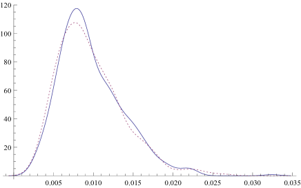
Figure 1. Kolmogorov-Smirnov distances between the empirical and true distribution for $X_{0}$. The solid line is for the reversal method starting $\zeta_{0}\sim p$ and the dashed line for the reversal method running $Z_{0}$ to $2T$ and setting $\zeta_{t}=Z_{2T-t}$. Here, $T=10,000$, $\delta=1/24$, $\gamma=2$ and $a=1$. Computations were performed using Mathematica and the code can be found on the author’s website www.math.cmu.edu/users/scottrob/research.

	Method A	Method B
Median Distance	0.00887	0.00882
Standard Deviation	0.00405	0.00413
$99^{th}$ Percentile	0.02168	0.02255
$1^{st}$ Percentile	0.00405	0.00290
Median Time (seconds)	2.694	8.766

Table 1. Statistics on Kolmogorov-Smirnov distances between the empirical and true distribution for $X_{0}$ using methods A and B.

Figure 1 shows the resulting Kolmogorov-Smirnov distances for $500$ sample paths. The plot gives a (smoothed) histogram comparing the distances using the two methods described above. As can be seen, the two methods give comparable results: this is not surprising given that rapid convergence of the distribution of $\zeta$ to its invariant distribution [9]. Table 1 provides summary statistics regarding the median distances and simulation times, as well as the standard deviation and tail data.

Having obtained Kolmogorov-Smirnov distances using reversal methods, we next compared our results to a naive simulation of $X_{0}$, obtained by sampling $Z_{0}\sim p$ and computing $X_{0}$ via (3.1) directly. Here, for the median distance $d$ using Method A from Table 1, we sampled $X_{0}$ stopping at the first instance $N$ so that the Kolmogorov-Smirnov distance between the empirical and true distribution for $X_{0}$ fell below $d$. As can be seen from Figure 2 and the summary statistics in Table 2, the naive simulation performs significantly worse: at the median it took $7,002$ paths and a simulation time of $8.66$ minutes to achieve the same level of accuracy as $1$ path ($2.94$ seconds) of the reversed process. Further, the histogram shows the presence of a significant number of trials where significantly more than the median number of paths were needed to achieve the given accuracy.

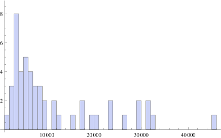
Figure 2. Histogram for the number $N$ of paths necessary so that, using the naive simulation for $X_{0}$, the Kolmogorov-Smirnov distance between the empirical distribution and true distribution for $X_{0}$ fell below the median distance $d$ using Method A from Table 1. The integral was computed using $T=100$ with mesh size of $\delta=1/24$; furthermore, the values $\gamma=2$ and $a=1$ we used. Computations were performed using Mathematica and the code can be found on the author’s website www.math.cmu.edu/users/scottrob/research.

Summary for the Forward Simulation
Median Number of Paths	7,002
Mean Number of Paths	11,446
Standard Deviation	10,165
Minimum Number of Paths	1,846
Maximum Number of Paths	45,004
Median Simulation Time (minutes)	8.66
Mean Simulation Time (minutes)	14.34

Table 2. Summary statistics using the naive forward simulation method.

4. Conclusion

In this work, using the method of time reversal, an efficient method for simulating the joint distribution of $(Z_{0},X_{0})$ for perpetuities of the form (0.1) is obtained. The joint distribution may be obtained by sampling a single path of the reversed process, as opposed to sampling numerous paths of $X_{0}$ using the naive method. However, the effectiveness of the proposed method depends on being to obtain analytic representations for the distribution $p$ of $Z_{0}$: an undertaking that, though always possible in the one-dimensional case, is often not possible for non-reversing multi-dimensional diffusions. Furthermore, results are presented for perpetuities with non-negative underlying cash flow rates. As such, more research is needed to identify an effective time reversal method for perpetuities of the form

$$X_{0}=\int_{0}^{\infty}D_{t}dF_{t}$$

for general Markovian processes $F$ (i.e., not just $dF_{t}=f(Z_{t})dt$) containing both jumps and diffusive terms. Additionally, the performance of the method where $Z$ is run until a large time $2T$ and then setting $\zeta_{t}=Z_{2T-t}$ must be thoroughly analyzed: in particular, how fast does the distribution of $Z_{2T}$ converge to $p$ given a fixed starting point? To answer these questions, one must first analyze the resultant backwards dynamics and associated PDEs for the invariant density, obtaining rates of convergence.

5. Proofs from Section 1.2

We present here the proofs of Lemma 1.3 and Lemma 1.5.

Proof of Lemma 1.3.

Let $\varepsilon>0$ be as in (1.4). Assume first that $\theta^{\prime}c\theta+\eta^{\prime}\eta\equiv 0$. Then $R=\int_{0}^{\cdot}a(Z_{t})\mathrm{d}t$ and (1.4) reads $a^{-}\in\mathbb{L}^{1}(E,p)$ and $\int_{E}a(z)p(z)\mathrm{d}z>0$. Set $\kappa\,:=\,(1/4)\int_{E}a(z)p(z)\mathrm{d}z>0$. Fix $z\in E$ and denote by $\mathbb{P}^{z}$ the probability obtained by conditioning upon $Z_{0}=z$. The positive recurrence of $Z$ implies ([28, Theorem 4.9.5]), there exists a $\mathbb{P}^{z}$-a.s. finite random variable $T(z)$ such that $t\geq T(z)$ implies that $R_{t}=\int_{0}^{t}a(Z_{u})\mathrm{d}u\geq 2\kappa t$ and hence the first conclusion of Lemma 1.3 holds. Furthermore, since $Z$ is stationary, ergodic under $\mathbb{P}$, the ergodic theorem implies there is a $\mathbb{P}$ a.s. finite random variable $T$ such that $t\geq T$ implies $R_{t}\geq 2\kappa t$. Now, let $n\in\mathbb{N}$ be such that $n>1/(2\kappa)$. We have

$$\sup_{t\geq 0}(t/n-R_{t})\leq\sup_{t\leq T}(t/n-R_{t})<\infty,$$

where the last inequality follows by the regularity of $a$ and the non-explositivity of $Z$. Thus

$$X_{0}=\int_{0}^{\infty}e^{-R_{t}}f(Z_{t})\mathrm{d}t\leq e^{\sup_{t\leq T}(t/n-R_{t})}\int_{0}^{\infty}e^{-t/n}f(Z_{t})\mathrm{d}t.$$

By the stationarity of $Z$:

$$\mathbb{E}\left[\int_{0}^{\infty}e^{-t/n}f(Z_{t})\mathrm{d}t\right]=\int_{0}^{\infty}e^{-t/n}\mathbb{E}\left[f(Z_{t})\right]\mathrm{d}t=n\int_{E}f(z)p(z)dz<\infty,$$

hence $\mathbb{P}\left[\int_{0}^{\infty}e^{-t/n}f(Z_{t})dt<\infty\right]=1$, which in turn implies that $\mathbb{P}\left[X_{0}<\infty\right]=1$.

Assume now that $\theta^{\prime}c\theta+\eta^{\prime}\eta\not\equiv 0$, which by continuity of all involved functions implies that $\int_{E}\left(\theta^{\prime}c\theta+\eta^{\prime}\eta\right)(z)p(z)\mathrm{d}z>0$. Fix $z\in E$. Positive recurrence of $Z$ gives that $\lim_{t\to\infty}\int_{0}^{t}(\theta^{\prime}c\theta+\eta^{\prime}\eta)(Z_{u})\mathrm{d}u=\infty$ with $\mathbb{P}^{z}$ probability one. On the event $\big{\{}\int_{0}^{t}(\theta^{\prime}c\theta+\eta^{\prime}\eta)(Z_{u})\mathrm{d}u>0\big{\}}$, note that

$$-R_{t}=-\int_{0}^{t}a(Z_{u})\mathrm{d}u+\int_{0}^{t}(\theta^{\prime}c\theta+\eta^{\prime}\eta)(Z_{u})\mathrm{d}u\left(-\frac{1}{2}-\frac{\int_{0}^{t}\theta^{\prime}\sigma(Z_{u})\mathrm{d}W_{u}+\eta(Z_{u})\mathrm{d}B_{u}}{\int_{0}^{t}(\theta^{\prime}c\theta+\eta^{\prime}\eta)(Z_{u})\mathrm{d}u}\right).$$

By the Dambis, Dubins and Schwarz theorem and the strong law of large numbers for Brownian motion, it follows that there exists a $\mathbb{P}^{z}$-a.s. finite random variable $T(z)$ such that

$$t\geq T(z)\quad\Longrightarrow\quad-\frac{\int_{0}^{t}\theta^{\prime}\sigma(Z_{u})\mathrm{d}W_{u}+\eta(Z_{u})\mathrm{d}B_{u}}{\int_{0}^{t}(\theta^{\prime}c\theta+\eta^{\prime}\eta)(Z_{u})\mathrm{d}u}\leq\frac{\varepsilon}{2};$$

therefore,

$$t\geq T(z)\quad\Longrightarrow\quad-R_{t}\leq-\int_{0}^{t}\left(a+\frac{1-\varepsilon}{2}(\theta^{\prime}c\theta+\eta^{\prime}\eta)\right)(Z_{u})\mathrm{d}u.$$

With $\kappa\,:=\,(1/4)\int_{E}(a+(1-\varepsilon)(\theta^{\prime}c\theta+\eta^{\prime}\eta)/2)(z)p(z)\mathrm{d}z>0$, and increasing $T(z)$ if necessary (still keeping it $\mathbb{P}^{z}$-a.s. finite), it follows that $t\geq T(z)$ implies $-R_{t}\leq-2\kappa t$. Hence the first part of Lemma 1.3 holds true again. Additionally, the ergodic theorem applied with $\mathbb{P}$ gives a $\mathbb{P}$-a.s. finite random variable $T$ such that $t\geq T$ implies $-R_{t}\leq-2\kappa t$. Again, for $n\in\mathbb{N}$ such that $n>1/(2\kappa)$ we have

$$X_{0}=\int_{0}^{\infty}e^{-R_{t}}f(Z_{t})\mathrm{d}t\leq e^{\sup_{t\leq T}(t/n-R_{t})}\int_{0}^{\infty}e^{-t/n}f(Z_{t})\mathrm{d}t.$$

from which $\mathbb{P}\left[X_{0}<\infty\right]=1$ follows by the same line of reasoning as above. ∎

Proof of Lemma 1.5.

The proof is nearly identical that if Lemma 1.3. Namely, in each of the cases $\theta^{\prime}c\theta+\eta^{\prime}\eta\equiv 0$ and $\theta^{\prime}c\theta+\eta^{\prime}\eta\not\equiv 0$, under the given hypothesis there is a constant $\kappa\geq 0$ and a $\mathbb{P}$-a.s. finite random variable $T$ such that $-R_{t}\geq\kappa t$ holds for $t\geq T$. This gives that

(5.1) $$X_{0}\geq\int_{T}^{\infty}e^{\kappa t}f(Z_{t})\mathrm{d}t\geq\int_{T}^{\infty}e^{\kappa t}(f\wedge N)(Z_{t})dt,$$

where $N$ is large enough so that $\int_{E}(f(z)\wedge N)p(z)\mathrm{d}z>0$. We thus have

$$X_{0}\geq\int_{0}^{\infty}e^{\kappa t}(f\wedge N)(Z_{t})dt-\frac{N}{\kappa}(e^{\kappa T}-1).$$

Ergodicity of $Z$ implies that $\mathbb{P}$ almost surely

$$\lim_{u\to\infty}\frac{1}{u}\int_{0}^{u}(f\wedge N)(Z_{t})\mathrm{d}t=\int_{E}\left(f(z)\wedge N\right)p(z)\mathrm{d}z>0,$$

so that $\lim_{u\to\infty}\int_{0}^{u}e^{\kappa t}(f\wedge N)(Z_{t})\mathrm{d}t=\infty$, proving the result. ∎

6. Proof of Theorem 2.1

Under the given assumptions there exists a unique solution, $(\mathbb{P}^{z,x})_{(z,x)\in F}$ to the generalized martingale problem for $L$ on $F$, where $L$ is from (2.5). Here, the measure space is $(\widetilde{\Omega},\widetilde{\mathbf{F}})$, where $\widetilde{\Omega}=(C[0,\infty);\hat{F})$, with $\hat{F}$ being the one-point compactification of $F$. The filtration $\widetilde{\mathbf{F}}$ is the right-continuous enlargement of the filtration generated by the coordinate process $(\widetilde{Z},\widetilde{Y})$ on $\widetilde{\Omega}$.

Let $(F_{n})_{n\in\mathbb{N}}$ be an increasing sequence smooth, bounded, open, connected domains of $F$ such that $F=\cup_{n}F_{n}$. Note that $F_{n}$ can be obtained by smoothing out the boundary of $E_{n}\times(1/n,n)$. By uniqueness of solutions to the generalized martingale problem, for each $n$, the law of of $(\widetilde{Z},\widetilde{Y})$ is the same as the law of $(Z,Y^{x})$ under $\mathbb{P}\left[\cdot\ |\ Z_{0}=z\right]$ (where the latter will always denote a version of the conditional probability) up until the first exit time of $F_{n}$. Furthermore, since the process $Z$ is recurrent, with $(\mathbb{P}^{z})_{z\in E}$ being the restriction of $(\mathbb{P}^{z,x})_{(z,x)\in F}$ to the first $d$ coordinates, for $z\in E$, the law of $\widetilde{Z}$ under $\mathbb{P}^{z}$ is the same as the law of $Z$ under $\mathbb{P}\left[\,\cdot\ |\ Z_{0}=z\right]$. For these reasons, and in order to ease the reading, we abuse notation and still use $(Z,Y)$ instead of $(\widetilde{Z},\widetilde{Y})$ for the coordinate process on $\widetilde{\Omega}$. The underlying space we are working on will be clear from the context.

Denote by $\tau_{n}$ the first exit time of $(Z,Y)$ from $F_{n}$. Assumption 1.7 implies $Z$ does not explode under $\mathbb{P}^{z,x}$ and $Y$ cannot explode to infinity since $D$ is strictly positive almost surely under $\mathbb{P}\left[\,\cdot\ |\ Z_{0}=z\right]$ for all $z\in E$. Therefore, the explosion time $\tau\,:=\,\lim_{n\to\infty}\tau_{n}$ for $(Z,Y)$ is the first hitting time of $Y$ to $0$ and the law of $\tau$ under $\mathbb{P}^{z,x}$ is the same as the law of the first hitting of $Y^{x}$ to $0$ under $\mathbb{P}\left[\,\cdot\ |\ Z_{0}=z\right]$.

Note that $Y^{x}_{t}=D_{t}^{-1}\left(x-X_{0}+\int_{t}^{\infty}D_{u}f(Z_{u})\mathrm{d}u\right)$. Assumption 1.7 implies

(6.1) $$\mathbb{P}\left[\int_{t}^{\infty}D_{u}f(Z_{u})\mathrm{d}u>0\ \Big{|}\ Z_{0}=z\right]=1,\qquad z\in E,\quad t\geq 0.$$

Therefore,

$$g(z,x)=\mathbb{P}\left[X_{0}\leq x\ |\ Z_{0}=z\right]=\mathbb{P}^{z,x}\left[Y^{x}_{t}>0,\ \forall t\geq 0\right]=\mathbb{P}^{z,x}\left[\tau=\infty\right].$$

Define

(6.2) $$h(z,x)\,:=\,\mathbb{P}^{z,x}\left[\lim_{t\to\infty}Y_{t}=\infty\right],\quad(z,x)\in F$$

Fix $(z,x)\in F$ and let $0<\varepsilon<x$. Note that $Y^{x}_{t}=Y^{x-\varepsilon}_{t}+\varepsilon/D_{t}$. Since $\lim_{t\to\infty}D_{t}=0$ holds $\mathbb{P}\left[\cdot\ |\ Z_{0}=z\right]$-a.s., it follows that

(6.3) $$\begin{split}\mathbb{P}^{z,x-\varepsilon}\left[\tau=\infty\right]&=\mathbb{P}\left[Y^{x-\varepsilon}_{t}>0\ \forall t\geq 0\ |\ Z_{0}=z\right]\\ &\leq\mathbb{P}\left[Y^{x}_{t}\geq\varepsilon/D_{t},\ \forall t\geq 0\ |\ Z_{0}=z\right]\\ &\leq\mathbb{P}\left[\lim_{t\to\infty}Y^{x}_{t}=\infty\ |\ Z_{0}=z\right]\\ &=\mathbb{P}^{z,x}\left[\lim_{t\to\infty}Y_{t}=\infty\right]\leq\mathbb{P}^{z,x}\left[\tau=\infty\right].\end{split}$$

Therefore, $g(z,x-\varepsilon)\leq h(z,x)\leq g(z,x)$. By definition, $g(z,x)$ is right-continuous in $x$ for a fixed $z$ and so

$$g(z,x)\leq\liminf_{\varepsilon\to 0}h(z,x+\varepsilon)\leq\limsup_{\varepsilon\to 0}h(z,x+\varepsilon)\leq\limsup_{\varepsilon\to 0}g(z,x+\varepsilon)=g(z,x).$$

Therefore, if $h(z,x)$ is continuous it follows that $h(z,x)=g(z,x)$. It is now shown that in fact $h$ is in $C^{2,\gamma}(F)$ and satisfies $Lh=0$. This gives the desired result for $g$ since $g=h$.

Let $\psi:(0,\infty)\mapsto(0,1)$ be a smooth function such that $\lim_{x\to 0}\psi(x)=0$, $\lim_{x\to\infty}\psi(x)=1$. By the classical Feynman-Kac formula

$$u^{n}(z,x)\,:=\,\mathbb{E}^{\mathbb{P}^{z,x}}\left[\psi(Y_{\tau_{n}})\right],$$

satisfies $Lu^{n}=0$ in $F_{n}$ with $u^{n}(z,x)=\psi(x)$ on $\partial F_{n}$. Since $\mathbb{P}\left[X_{0}<\infty\ |\ Z_{0}=z\right]=1$ there exists a pair $(z_{0},x_{0})\in F$ so that $\mathbb{P}\left[X_{0}<x_{0}\ |\ Z_{0}=z_{0}\right]>0$. Using (6.3) this gives

(6.4) $$h(z_{0},x_{0})\geq\mathbb{P}\left[X_{0}<x_{0}\ |\ Z_{0}=z_{0}\right]>0.$$

Therefore, $(\mathbb{P}^{z,x})_{(z,x)\in F}$ is transient [28, Chapter 2] and, since $(\mathbb{P}^{z})_{z\in E}$ is positive recurrent, this implies that for all $(z,x)$, with $\mathbb{P}^{z,x}$-probability one, either $\lim_{t\to\tau}Y_{t}=0$ or $\lim_{t\to\tau}Y_{t}=\infty$, where in the latter case, $\tau=\infty$ since $Y$ cannot explode to $\infty$. This in turn yields that $Y_{\tau_{n}}\rightarrow 0$ or $Y_{\tau_{n}}\rightarrow\infty$ with $\mathbb{P}^{z,x}$-probability one and hence by the dominated convergence theorem

(6.5) $$\lim_{n\to\infty}u^{n}(z,x)=\mathbb{P}^{z,x}\left[\lim_{t\to\tau}Y_{t}=\infty\right]=\mathbb{P}^{z,x}\left[\lim_{t\to\infty}Y_{t}=\infty\right]=h(z,x).$$

For $(z_{0},x_{0})$ from (6.4), $g(z_{0},x_{0})\geq h(z_{0},x_{0})>0$ and hence $g(z,x)>0$ for all $(z,x)\in F$ [28, Theorem 1.15.1]. But this implies $h(z,x)\geq g(z,x/2)>0$, and so from (6.5) the $u^{n}$ are converging point-wise to a strictly positive function. Thus, by the interior Schauder estimates and Harnack’s inequality, it follows by “the standard compactness” argument ([28, Page 147]) that there exists a $C^{2,\gamma}(F)$, strictly positive, function $u$ such that $u^{n}$ converges to $u$ in the $C^{2,\gamma}(D)$ Holder space for all compact $D\subset F$. Clearly, this function $u$ satisfies $Lu=0$ in $F$. In fact, since $u^{n}$ converges to $h$ pointwise, $h=u$ and hence $Lh=0$.

The boundary conditions for $g$ are now considered. Let the integer $k$ be given. It suffices to show for each $\varepsilon>0$ there is some $n(\varepsilon)$ such that

(6.6) $$\sup_{x\leq n(\varepsilon)^{-1},z\in E_{k}}g(z,x)\leq\varepsilon;\qquad\inf_{x\geq n(\varepsilon),z\in E_{k}}g(z,x)\geq 1-\varepsilon$$

The condition near $x=0$ is handled first. By way of contradiction, assume there exists some $\varepsilon>0$ such that for all integers $n$ there exists $z_{n}\in E_{k}$, $x_{n}\leq 1/n$ such that $g(z_{n},x_{n})>\varepsilon$. Since the $z_{n}$ are all contained within $E_{k}$ there is a sub-sequence (still labeled $n$) such that $z_{n}\rightarrow z$ for $z\in\bar{E}_{k}$.

Let $\delta>0$ and choose $N_{\delta}$ such that $n\geq N_{\delta}$ implies $n^{-1}\leq\delta$. Since $g$ is increasing in $x$, $\varepsilon<g(z_{n},\delta)$. Since $g$ is continuous, $\varepsilon\leq g(z,\delta)$. Since this is true for all $\delta>0$, $\lim_{x\to 0}g(z,x)\geq\varepsilon$. But, this is a contradiction : $\lim_{x\to 0}g(z,x)=0$ for each $z\in E$. To see this, let $\delta>0$ and choose $\beta>0$ such that $\mathbb{P}\left[X_{0}\geq\beta\ |\ Z_{0}=z\right]\geq 1-\delta$. This is possible in view of (6.1). Thus, for $x<\beta$, $g(z,x)\leq\mathbb{P}\left[X_{0}<\beta\ |\ Z_{0}=z\right]\leq\delta$ and hence $\limsup_{x\to 0}g(z,x)\leq\delta$. Taking $\delta\to 0$ gives the result.

The proof for $x\to\infty$ is very similar. Assume by contradiction that there is some $\varepsilon>0$ such that for all integers $n$ there exist $z_{n}\in E_{k}$, $x_{n}\geq n$ such that $g(z_{n},x_{n})<1-\varepsilon$. Again, by taking sub-sequences, it is possible to assume $z_{n}\rightarrow z\in\bar{E}_{k}$. Fix $M>0$. For $n\geq M$, since $g$ is increasing in $x$, $g(z_{n},M)<1-\varepsilon$. Since $g$ is continuous, $g(z,M)\leq 1-\varepsilon$. Since this holds for all $M$, $\lim_{x\to\infty}g(z,x)\leq 1-\varepsilon$. But, this violates the condition that under $\mathbb{P}\left[\cdot\ |\ Z_{0}=z\right]$, $X_{0}<\infty$ almost surely.

The uniqueness claim is now proved. Let $\tilde{g}$ be a $C^{2}(F)$ solution of $L\tilde{g}=0$ such that $0\leq\tilde{g}\leq 1$ and such that (2.6) holds. Define the stopping times

(6.7) $$\sigma_{k}\,:=\,\inf\left\{t\geq 0:Z_{t}\not\in E_{k}\right\};\qquad\rho_{k}\,:=\,\inf\left\{t\geq 0:Y_{t}=k\right\}.$$

By Ito’s formula, for any $k,n,m$

$$\begin{split}\tilde{g}(z,x)&=\mathbb{E}^{\mathbb{P}^{z,x}}\left[g(Z_{\sigma_{k}\wedge\rho_{1/n}\wedge\rho_{m}},Y_{\sigma_{k}\wedge\rho_{1/n}\wedge\rho_{m}})\left(1_{\rho_{1/n}<\sigma_{k}\wedge\rho_{m}}+1_{\rho_{1/n}\geq\sigma_{k}\wedge\rho_{m}}(1_{\tau<\infty}+1_{\tau=\infty})\right)\right].\end{split}$$

Since $\mathbb{P}^{z,x}$ almost surely $\lim_{m\to\infty}\rho_{m}=\infty$, taking $m\to\infty$ yields

$$\begin{split}\tilde{g}(z,x)&=\hat{\mathbb{E}}^{\mathbb{P}^{z,x}}\left[g(Z_{\sigma_{k}\wedge\rho_{1/n}},Y_{\sigma_{k}\wedge\rho_{1/n}})\left(1_{\rho_{1/n}<\sigma_{k}}+1_{\rho_{1/n}\geq\sigma_{k}}(1_{\tau<\infty}+1_{\tau=\infty})\right)\right].\end{split}$$

On $\left\{\rho_{1/n}<\sigma_{k}\right\}$, $Z_{\rho_{1/n}}\in E_{k}$, $Y_{\rho_{1/n}}\leq 1/n$ and hence by $0\leq\tilde{g}\leq 1$ and (2.6), for any $\varepsilon>0$ there is an $n(\varepsilon)$ such that for $n\geq n(\varepsilon)$

$$\begin{split}\tilde{g}(z,x)&\leq\varepsilon+\mathbb{P}^{z,x}\left[\rho_{1/n}\geq\sigma_{k},\tau<\infty\right]+\mathbb{P}^{z,x}\left[\rho_{1/n}\geq\sigma_{k},\tau=\infty\right].\end{split}$$

Taking $n\to\infty$ thus gives

$$\begin{split}\tilde{g}(z,x)&\leq\varepsilon+\mathbb{P}^{z,x}\left[\tau\geq\sigma_{k},\tau<\infty\right]+\mathbb{P}^{z,x}\left[\tau=\infty\right].\end{split}$$

Taking $k\to\infty$ gives

$$\begin{split}\tilde{g}(z,x)&\leq\varepsilon+\mathbb{P}^{z,x}\left[\tau=\infty\right].\end{split}$$

and hence taking $\varepsilon\to 0$ gives $\tilde{g}(z,x)\leq\mathbb{P}^{z,x}\left[\tau=\infty\right]=g(z,x)$. Similarly, for $k,n,m$

$$\begin{split}\tilde{g}(z,x)&=\mathbb{E}^{\mathbb{P}^{z,x}}\left[g(Z_{\sigma_{k}\wedge\rho_{1/n}\wedge\rho_{m}},Y_{\sigma_{k}\wedge\rho_{1/n}\wedge\rho_{m}})\left(1_{\rho_{m}<\sigma_{k}\wedge\rho_{1/n}}+1_{\rho_{m}\geq\sigma_{k}\wedge\rho_{1/n}}\right)\right],\\ &\geq(1-\varepsilon)\hat{\mathbb{P}}^{z,x}\left[\rho_{m}<\sigma_{k}\wedge\rho_{1/n},\lim_{t\to\infty}Y_{t}=\infty\right],\end{split}$$

for all $\varepsilon>0$ and $m\geq m(\varepsilon)$ for some $m(\varepsilon)$. Note that the set $\left\{\rho_{m}<\sigma_{k}\wedge\rho_{1/n}\right\}$ is restricted to include $\left\{\lim_{t\to\infty}Y_{t}=\infty\right\}$ but this is fine since lower bounds are considered. Now, on the event $\left\{\lim_{t\to\infty}Y_{t}=\infty\right\}$ it holds that $\rho_{1/n}\rightarrow\infty$. Thus, taking $n\to\infty$

$$\tilde{g}(z,x)\geq(1-\varepsilon)\mathbb{P}^{z,x}\left[\rho_{m}<\sigma_{k},\lim_{t\to\infty}Y_{t}=\infty\right].$$

Taking $k\to\infty$ gives

$$\tilde{g}(z,x)\geq(1-\varepsilon)\mathbb{P}^{z,x}\left[\rho_{m}<\infty,\lim_{t\to\infty}Y_{t}=\infty\right].$$

Taking $m\to\infty$ and noting that for $m$ large enough $\rho_{m}<\infty$ on $\lim_{t\to\infty}Y_{t}=\infty$ it holds that

$$\tilde{g}(z,x)\geq(1-\varepsilon)\mathbb{P}^{z,x}\left[\lim_{t\to\infty}Y_{t}=\infty\right]=(1-\varepsilon)h(z,x).$$

where the last equality follows by the definition of $h$ in (6.2). Now, in proving $Lg=0$ it was shown that $g=h$ and hence $\tilde{g}(z,x)\geq(1-\varepsilon)g(z,x)$. Taking $\varepsilon\to 0$ gives that $\tilde{g}(z,x)\geq g(z,x)$, finishing the proof.

7. Dynamics for the Time-Reversed Process

The goal of the next two sections is to prove Theorem 2.4. We keep all notation from Subsection 2.2. We first identify the dynamics for $\zeta^{T}$.

Proposition 7.1.

Let Assumptions 1.7 hold. Then, for each $T>0$, the law of $\zeta^{T}$ under $\mathbb{P}$ solves the martingale problem on $E$ (for $t\leq T$) for the operator $L^{\zeta}\,:=\,(1/2)c^{ij}\partial^{2}_{ij}+\mu^{i}\partial_{i}$ where

(7.1) $$\mu\,:=\,c\frac{\nabla p}{p}+\textrm{div}\left(c\right)-m.$$

The operator $L^{\zeta}$ does not depend upon $T$. Thus, if $\left(\mathbb{Q}^{z}\right)_{z\in E}$ denotes the solution of the generalized martingale problem for $L^{\zeta}$ on $E$, then in fact $(\mathbb{Q}^{z})_{\zeta\in E}$ solves the martingale problem for $L^{\zeta}$ on $E$ and is positive recurrent.

Remark 7.2.

If $Z$ is reversing then $p$ satisfies $m=(1/2)\left(c\nabla{p}/p+\textrm{div}\left(c\right)\right)$. Thus, in this instance, $\mu=m$ and, as the name suggests, $\zeta^{T}$ has the same dynamics as $Z$.

Proof.

The first statement regarding the martingale problem is based off the argument in [20]. Since $Z$ is positive recurrent with invariant measure $p$ and $Z_{0}$ has initial distribution $p$ under $\mathbb{P}$, $Z$ is stationary with distribution $p$. Since $\tilde{L}^{Z}p=0$, equation $(2.5)$ in [20] holds noting that $p$ does not depend upon $t$.

For a given $s\leq t\leq t$ and $g\in C^{\infty}_{c}(E)$ define the function $v(s,z)\,:=\,\mathbb{E}\left[g(X_{t})\big{|}Z_{s}=z\right]$. The Feynman-Kac formula implies $v$ satisfies $v_{s}+L^{z}v=0$ on $0<s<t,z\in E$ with $v(t,z)=g(z)$ : see [21, 19] for an extension of the classical Feynman-Kac formula to the current setup. Therefore, the condition in equation $(2.7)$ of [20] holds as well. Thus, the formal argument on page $1191$ of [20] is rigorous and the law of $\zeta^{T}$ under $\mathbb{P}$ solves the martingale problem for $L^{\zeta}$.

Turning to the statement regarding $\left(\mathbb{Q}^{z}\right)_{z\in E}$, set $\tilde{L}^{\zeta}$ as the formal adjoint to $L^{\zeta}$. $\tilde{L}^{\zeta}$ is given by (1.2) with $\mu$ replacing $m$ therein. Using the formula for $\mu$ in (7.1) and for $\tilde{L}^{Z}$ in (1.2) calculation shows that

$$\tilde{L}^{\zeta}f=\tilde{L}^{Z}f-2\nabla\cdot\left(\frac{f}{p}\left(\frac{1}{2}\left(c\nabla p+p\textrm{div}\left(c\right)\right)-pm\right)\right).$$

Since

(7.2) $$0=\tilde{L}^{Z}p=\nabla\cdot\left(\frac{1}{2}\left(c\nabla p+p\textrm{div}\left(c\right)\right)-pm\right),$$

it follows by considering $f=p$ above that $\tilde{L}^{\zeta}p=0$. Therefore, $p$ is an invariant density for $L^{\zeta}$ if an only if the diffusion corresponding to the operator $\tilde{L}^{\zeta,p}$ does not explode, where $\tilde{L}^{\zeta,p}$ is the h-transform of $\tilde{L}^{\zeta}$ [28, Theorem 4.8.5]. But, by definition of the h-transform [28, pp. 126] and (1.2) with $\mu$ replacing $m$:

$$\begin{split}\tilde{L}^{\zeta,p}f&\,:=\,\frac{1}{p}\tilde{L}^{\zeta}(fp)=\frac{1}{2}c^{ij}\partial^{2}_{ij}f-\left(\mu^{i}-\textrm{div}\left(c\right)^{i}-\left(c\frac{\nabla p}{p}\right)^{i}\right)\partial_{i}f+\frac{f}{p}\tilde{L}^{\zeta}p,\\ &=\frac{1}{2}c^{ij}\partial^{2}_{ij}f+m^{i}\partial_{i}f=L^{Z}f,\end{split}$$

where the third equality follows from (7.1). Thus, Assumption 1.7 (specifically the fact that $Z$ is ergodic and $\int_{E}p(z)dz=1$) implies the diffusion for $\tilde{L}^{\zeta,p}$ not only does not explode but also is positive recurrent, finishing the proof. ∎

In preparation for the proof of the main result of this Section, which is Proposition 7.5, it is first needed to define a certain “backwards” filtration $\mathbf{G}^{T}$ and to present two Lemmas. Fix $T\in(0,\infty)$ and $t\in[0,T]$ and let $\widetilde{\mathcal{G}}^{T}_{t}$ be the $\sigma$-field generated by $X_{T}$, $(Z_{T-u})_{u\in[0,t]}$, $(W_{T}-W_{T-u})_{u\in[0,t]}$ and $(B_{T}-B_{T-u})_{u\in[0,t]}$. Then, let $\mathbf{G}^{T}\,:=\,(\mathcal{G}^{T}_{t})_{t\in[0,T]}$ be the usual augmentation of $(\widetilde{\mathcal{G}}^{T}_{t})_{t\in[0,T]}$. It is easy to check that $(\chi^{T},\zeta^{T})$ is $\mathbf{G}^{T}$-adapted for all $T\in\mathbb{R}_{+}$, as well as that the process $B^{T}$ defined via $B^{T}_{t}\,:=\,B_{T-t}-B_{T}$ is a $k$ dimensional Brownian motion on $(\Omega,\mathbf{G}^{T},\mathbb{P})$, independent of $(\chi^{T}_{0},\zeta^{T}_{0})=(X_{T},Z_{T})$. However, the $\mathbf{G}^{T}$-adapted process $(W_{T-t}-W_{T})_{t\in[0,T]}$ is not necessarily a Brownian motion on $(\Omega,\mathbf{G}^{T},\mathbb{P})$.

With this notation, the following two Lemmas are essential for proving Proposition 7.5.

Lemma 7.3.

Let Assumptions 1.7 hold. For locally bounded Borel function $\eta:E\mapsto\mathbb{R}$ and $0\leq s\leq t\leq T$, it holds that

(7.3) $$-\int_{T-t}^{T-s}\eta(Z_{u})^{\prime}\mathrm{d}B_{u}=\int_{s}^{t}\eta(\zeta^{T}_{u})^{\prime}\mathrm{d}B^{T}_{u}.$$

Furthermore, if $\theta:E\mapsto\mathbb{R}^{d}$ is continuously differentiable, then

(7.4) $$-\int_{T-t}^{T-s}\theta^{\prime}(Z_{u})\mathrm{d}Z_{u}=\int_{s}^{t}\theta^{\prime}(\zeta^{T}_{u})\mathrm{d}\zeta^{T}_{u}+\int_{s}^{t}\left(\nabla\cdot(c\theta)-\theta^{\prime}\textrm{div}\left(c\right)\right)(\zeta^{T}_{u})\mathrm{d}u.$$

Proof.

Fix $0\leq s\leq t\leq T$. For each $n\in\mathbb{N}$ and $i\in\left\{0,\ldots,n\right\}$, let

(7.5) $$u^{n}_{i}\,:=\,T-t+i(t-s)/n.$$

First, assume that $\eta$ is twice continuously differentiable. The standard convergence theorem for stochastic integrals implies that (the following limit is to be understood in measure $\mathbb{P}$):

$$\int_{s}^{t}\eta(\zeta^{T}_{u})^{\prime}\mathrm{d}B^{T}_{u}+\int_{T-t}^{T-s}\eta(Z_{u})^{\prime}\mathrm{d}B_{u}=-\lim_{n\to\infty}\left(\sum_{i=1}^{n}\left(\eta(Z_{u^{n}_{i}})-\eta(Z_{u^{n}_{i-1}})\right)^{\prime}\left(B_{u^{n}_{i}}-B_{u^{n}_{i-1}}\right)\right).$$

Since $B$ and $Z$ are independent, by Ito’s formula the last quadratic covariation is zero. Therefore, (7.3) holds for twice continuously differentiable $\eta$. The fact that (7.3) holds whenever $\eta$ is locally bounded follows from a monotone class argument.

In a similar manner, assume that $\theta$ is twice continuously differentiable. The standard convergence theorem for stochastic integrals implies that

$$\int_{s}^{t}\theta^{\prime}(\zeta^{T}_{u})\mathrm{d}\zeta^{T}_{u} +\int_{T-t}^{T-s}\theta^{\prime}(Z_{u})\mathrm{d}Z_{u}=-\lim_{n\to\infty}\left(\sum_{i=1}^{n}\left(\theta(Z_{u^{n}_{i}})-\theta(Z_{u^{n}_{i-1}})\right)^{\prime}(Z_{u^{n}_{i}}-Z_{u^{n}_{i-1}})\right).$$

The last quadratic covariation process (without the minus sign) is equal to

$$\int_{T-t}^{T-s}\tilde{F}(c,\theta)(Z_{u})\mathrm{d}u=\int_{s}^{t}\tilde{F}(c,\theta)(\zeta^{T}_{u})\mathrm{d}u,$$

where $\tilde{F}(c,\theta):E\mapsto\mathbb{R}$ is given by

$$\tilde{F}(c,\theta)=\sum_{i,j=1}^{d}c^{ij}\partial_{z_{i}}\theta^{j}=\sum_{i,j=1}^{d}\left(\partial_{z_{i}}(c^{ij}\theta^{j})-\theta^{j}\partial_{z_{i}}((c^{\prime})^{ji})\right)=\nabla\cdot(c\theta)-\theta^{\prime}\textrm{div}\left(c\right),$$

since $c^{\prime}=c$. Thus, (7.4) is established in the case where $\theta$ is twice continuously differentiable. The fact that (7.4) holds whenever $\theta$ is continuously differentiable follows form a density argument, noting that there exists a sequence $(\theta_{n})_{n\in\mathbb{N}}$ of polynomials such that $\lim_{n\to\infty}\theta_{n}=\theta$ and $\lim_{n\to\infty}\nabla\theta_{n}=\nabla\theta$ both hold, where the convergence is uniform on compact subsets of $E$. ∎

Lemma 7.4.

Let Assumptions 1.7 hold. For each $T\in\mathbb{R}_{+}$, define the $\mathbf{G}^{T}$-adapted continuous-path $\Delta^{T}$ as in (2.9). Then $\Delta^{T}$ is a semimartingale on $(\Omega,\mathbf{G}^{T},\mathbb{P})$. More precisely, for $t\in[0,T]$

(7.6) $$\begin{split}\Delta^{T}_{t}&=1+\int_{0}^{t}\Delta^{T}_{u}\left(\theta^{\prime}c\frac{\nabla p}{p}+\nabla\cdot(c\theta)-a\right)(\zeta^{T}_{u})\mathrm{d}u\\ &\qquad\qquad+\int_{0}^{t}\Delta^{T}_{u}\left(\eta(\zeta^{T}_{u})^{\prime}\mathrm{d}B^{T}_{u}+\theta^{\prime}\sigma(\zeta^{T}_{u})\mathrm{d}W^{T}_{u}\right).\end{split}$$

Proof.

Define $(\rho^{T}_{t})_{t\in[0,T]}$ by $\rho^{T}_{t}\,:=\,R_{T}-R_{T-t}$, for $t\in[0,T]$. In view of (0.2), (1.3), (7.1) and Lemma 7.3,

$$\rho^{T} =\int_{T-\cdot}^{T}\left(a+\frac{1}{2}(\theta^{\prime}c\theta+\eta^{\prime}\eta)\right)(Z_{t})\mathrm{d}t+\int_{T-\cdot}^{T}\left(\eta(Z_{t})^{\prime}\mathrm{d}B_{t}+\theta^{\prime}\sigma(Z_{t})\mathrm{d}W_{t}\right)$$

$$=\int_{T-\cdot}^{T}\left(a-\theta^{\prime}m+\frac{1}{2}(\theta^{\prime}c\theta+\eta^{\prime}\eta)\right)(Z_{t})\mathrm{d}t+\int_{T-\cdot}^{T}\left(\eta(Z_{t})^{\prime}\mathrm{d}B_{t}+\theta^{\prime}(Z_{t})\mathrm{d}Z_{t}\right)$$

$$=\int_{0}^{\cdot}\left(a-\theta^{\prime}m+\theta^{\prime}\textrm{div}\left(c\right)-\nabla\cdot(c\theta)+\frac{1}{2}(\theta^{\prime}c\theta+\eta^{\prime}\eta)\right)(\zeta^{T}_{t})\mathrm{d}t-\int_{0}^{\cdot}\left(\eta(\zeta^{T}_{t})^{\prime}\mathrm{d}B^{T}_{t}+\theta^{\prime}(\zeta^{T}_{t})\mathrm{d}\zeta^{T}_{t}\right),$$

$$=\int_{0}^{\cdot}\left(a-\theta^{\prime}c\frac{\nabla p}{p}-\nabla\cdot(c\theta)+\frac{1}{2}(\theta^{\prime}c\theta+\eta^{\prime}\eta)\right)(\zeta^{T}_{t})\mathrm{d}t-\int_{0}^{\cdot}\left(\eta(\zeta^{T}_{t})^{\prime}\mathrm{d}B^{T}_{t}+\theta^{\prime}\sigma(\zeta^{T}_{t})\mathrm{d}W^{T}_{t}\right).$$

The fact that $D=\exp(-R)$ gives $\Delta^{T}=\exp(-\rho^{T})$. Then, the dynamics for $\Delta^{T}$ follow from the dynamics of $\rho^{T}$. ∎

Proposition 7.5.

Let Assumptions 1.7 hold. Then, for each $T>0$ there is a filtration $\mathbf{G}^{T}$ satisfying the usual conditions and $d$ and $k$ dimensional independent $(\mathbb{P},\mathbf{G}^{T})$ Brownian motions $W^{T},B^{T}$ on $[0,T]$ so that the pair $(\zeta^{T},\chi^{T})$ have dynamics

(7.7) $$\begin{split}\zeta^{T}_{t}&=\zeta^{T}_{0}+\int_{0}^{T}\left(c\frac{\nabla p}{p}+\textrm{div}\left(c\right)-m\right)(\zeta^{T}_{u})\mathrm{d}u+\int_{0}^{T}\sigma(\zeta^{T}_{u})\mathrm{d}W^{T}_{u},\\ \chi^{T}_{t}&=\chi^{T}_{0}+\int_{0}^{T}\left(f(\zeta^{T}_{u})-\chi^{T}_{u}\left(a-\theta^{\prime}c\frac{\nabla p}{p}-\nabla\cdot(c\theta)\right)(\zeta^{T}_{u})\right)\mathrm{d}u\\ &\qquad\qquad+\int_{0}^{T}\chi^{T}_{u}\left(\theta^{\prime}\sigma(\zeta^{T}_{u})\mathrm{d}W^{T}_{u}+\eta(\zeta^{T}_{u})^{\prime}\mathrm{d}B^{T}_{u}\right).\end{split}$$

Proof of Proposition 7.5.

Proposition 7.1 immediately implies that under $\mathbb{P}$, $\zeta^{T}$ has dynamics:

(7.8) $$\begin{split}\zeta^{T}_{t}&=\zeta^{T}_{0}+\int_{0}^{t}\left(c\frac{\nabla p}{p}+\textrm{div}\left(c\right)-m\right)(\zeta^{T}_{u})du+\int_{0}^{t}\sigma(\zeta^{T}_{u})dW^{T}_{u};\qquad t\in[0,T],\end{split}$$

where $(W^{T}_{t})_{t\in[0,T]}$ is a Brownian motion on $(\Omega,\mathbf{G}^{T},\mathbb{P})$. In order to specify the dynamics for $\chi^{T}$, recall the definition of $\Delta^{T}$ from (2.9). Observe that

$$X_{T-t}=\frac{1}{D_{T-t}}\int_{T-t}^{\infty}D_{u}f(Z_{u})\mathrm{d}u=\frac{D_{T}}{D_{T-t}}\left(X_{T}+\int_{T-t}^{T}\frac{D_{u}}{D_{T}}f(Z_{u})\mathrm{d}u\right);\qquad t\in[0,T].$$

Then, using the definitions of $\chi^{T}$, $\zeta^{T}$ and $\Delta^{T}$, the above is rewritten as

(7.9) $$\chi^{T}_{t}=\Delta_{t}^{T}\left(\chi^{T}_{0}+\int_{0}^{t}\frac{1}{\Delta^{T}_{u}}f(\zeta^{T}_{u})\mathrm{d}u\right);\qquad t\in[0,T].$$

Lemma 7.4 implies $\Delta^{T}$ is a semimartingale, and hence (7.9) yields

$$\chi^{T}_{t}=\chi^{T}_{0}+\int_{0}^{t}\chi^{T}_{u}\,\frac{\mathrm{d}\Delta_{u}^{T}}{\Delta_{u}^{T}}+\int_{0}^{t}f(\zeta^{T}_{u})\mathrm{d}u;\qquad t\in[0,T].$$

The result now follows by plugging in for $\mathrm{d}\Delta^{T}_{u}/\Delta^{T}_{u}$ from (7.6). ∎

8. Proof of Theorem 2.4

8.1. Preliminaries

We first prove two technical results. The first asserts the existence of a probability space and stationary processes $(\zeta,\chi)$ consistent with $(\zeta,\chi^{x})$ in Theorem 2.4 in that given $\chi_{0}=x$, it holds that $\chi_{t}=\chi^{x}_{t},t\geq 0$. The second proposition shows that under the non-degeneracy assumption $|\eta|(z)>0,z\in E$ and regularity assumption $f\in C^{2}(E;\mathbb{R}_{+})$ it follows that $(\zeta,\chi)$ is ergodic.

Lemma 8.1.

Let Assumption 1.7 hold. Then, there is a filtered probability space $\left(\Omega,\mathbf{F},\mathbb{Q}\right)$, supporting independent $d$ and $k$ dimensional Brownian motions $W$ and $B$, $\mathcal{F}_{0}$ measurable random variables $\zeta_{0},\chi_{0}$ with joint distribution $\pi$, as well as a stationary process $\zeta$ with dynamics

(8.1) $$\zeta=\zeta_{0}+\int_{0}^{\cdot}\left(c\frac{\nabla p}{p}+\textrm{div}\left(c\right)-m\right)(\zeta_{t})\mathrm{d}t+\int_{0}^{\cdot}\sigma(\zeta_{t})\mathrm{d}W_{t}.$$

Furthermore, with $\Delta,\chi^{x}$ defined as in (2.12), (2.13), if the process $\chi$ is defined by $\chi_{t}\,:=\,\chi^{\chi_{0}}_{t}$ (see Remark 2.5) then $(\zeta,\chi)$ are stationary with invariant measure $\pi$ and joint dynamics

(8.2) $$\begin{split}\mathrm{d}\zeta_{t}&=\left(c\frac{\nabla p}{p}+\textrm{div}\left(c\right)-m\right)(\zeta_{t})\mathrm{d}t+\sigma(\zeta_{t})\mathrm{d}W_{t},\quad t\in\mathbb{R}_{+},\\ \mathrm{d}\chi_{t}&=\left(f(\zeta_{t})-\chi_{t}\left(a-\theta^{\prime}c\frac{\nabla p}{p}-\nabla\cdot(c\theta)\right)(\zeta_{t})\right)\mathrm{d}t+\chi_{t}\left(\theta^{\prime}\sigma(\zeta_{t})\mathrm{d}W_{t}+\eta(\zeta_{t})^{\prime}\mathrm{d}B_{t}\right),\quad t\in\mathbb{R}_{+}.\end{split}$$

Proof.

This result follows from Proposition 7.1. Indeed, one can start with a probability space $\left(\Omega,\mathbf{F},\mathbb{Q}\right)$ supporting independent $d$ and $k$ dimensional Brownian motions $W$ and $B$ respectively, as well as a $\mathcal{F}_{0}$ measurable random variable $(\zeta_{0},\chi_{0})\sim\pi$ (hence independent of $W$ and $B$). Under the given regularity assumptions, Proposition 7.1 yields a strong, stationary solution $\zeta$ satisfying (8.1). Then, defining $\Delta$ as in (2.9) and, for $x>0$, $\chi^{x}$ as in (2.13), it follows that $(\zeta,\chi^{x})$ and hence $(\zeta,\chi)$ satisfy the SDE in (8.2). Under the given regularity assumptions the law under $\mathbb{P}$ of $(\zeta^{T},\chi^{T})$ given $\zeta^{T}_{0}=z,\chi^{T}_{0}=x$ coincides with the law under $\mathbb{Q}$ of $(\zeta,\chi^{x})$ given that $\zeta_{0}=z$. Since by construction, $\pi$ is an invariant measure for $(\zeta^{T},\chi^{T})$, it follows from the Markov property that $\pi$ is invariant for $(\zeta,\chi)$ under $\mathbb{Q}$ and hence $(\zeta,\chi)$ is stationary with invariant measure $\pi$. ∎

Define the measures $\mathbb{Q}^{z,x}$ for $(z,x)\in F$ via

(8.3) $$\mathbb{Q}^{z,x}\left[A\right]=\mathbb{Q}\left[A\ |\ \zeta_{0}=z,\chi_{0}=x\right];\qquad A\in\mathcal{F}_{\infty}$$

We now consider when $|\eta|>0$ on $E$ and $f\in C^{2}(E;\mathbb{R}_{+})$. According to Theorem 2.1, $g\in C^{2,\gamma}(F)$ and hence $\pi$ possesses a density satisfying

(8.4) $$\pi(z,x)=p(z)\partial_{x}g(z,x);\qquad(z,x)\in F.$$

Additionally, we have the following Proposition:

Proposition 8.2.

Let Assumption 1.7 hold, and additionally suppose that $|\eta|(z)>0$ for $z\in E$ and $f\in C^{2}(E;\mathbb{R}_{+})$. Then the process $(\zeta,\chi)$ from Lemma 8.1 is ergodic. Thus, for all bounded measurable functions $h$ on $F$ and all $(z,x)\in F$

(8.5) $$\lim_{T\to\infty}\frac{1}{T}\int_{0}^{T}h(\zeta_{t},\chi_{t})dt=\int_{F}hd\pi;\quad\mathbb{Q}^{z,x}\textrm{a.s.}.$$

Proof of Proposition 8.2.

Recall $A$ from (2.4) and define $b^{R}:F\mapsto\mathbb{R}^{d+1}$ by

(8.6) $$\begin{split}b^{R}(z,x)\,:=\,\left(\begin{array}[]{c}\left(c(\nabla p/p)+\textrm{div}\left(c\right)-m\right)(z)\\ f(z)-x\left(a-\theta^{\prime}c\left(\nabla p/p\right)-\nabla\cdot(c\theta)\right)(z)\end{array}\right).\end{split}$$

From (8.2) it is clear that the generator for $(\zeta,\chi)$ is $L^{R}\,:=\,(1/2)A^{ij}\partial^{2}_{ij}+(b^{R})^{i}\partial_{i}$. As an abuse of notation, let $(\mathbb{Q}^{z,x})_{(z,x)\in F}$ also denote the solution to the generalized martingale problem for $L^{R}$ on $F$. Using Theorem 2.1, and the fact that under the given coefficient regularity assumptions, $g\in C^{3}(F)$ (see [16, Ch. 6]) a lengthy calculation performed in Lemma A.1 below shows that the density $\pi$ from (8.4) solves $\tilde{L}^{R}\pi=0$ where $\tilde{L}^{R}$ is the formal adjoint to $L$. Since by construction, $\iint_{F}\pi(z,x)dzdx=1$, positive recurrence will follow once it is shown that $(\mathbb{Q}^{z,x})_{(z,x)\in F}$ is recurrent. By Proposition 7.1, the restriction of $\mathbb{Q}^{z,x}$ to the first $d$ coordinates (i.e. the part for $\zeta$) is positive recurrent. Since by (2.13) it is evident that $\chi$ does not hit $0$ in finite time, it follows that that $\chi$ does not explode under $\mathbb{Q}^{z,x}$. Thus, [28, Corollary 4.9.4] shows that $(\zeta,\chi)$ is recurrent. Now, that (8.5) holds follows from [28, Theorem 4.9.5].

∎

8.2. Proof of Theorem 2.4

The proof of Theorem 2.4 uses a number of approximations arguments. To make these arguments precise, we first enlarge the original probability space $(\Omega,\,\mathbf{F},\,\mathbb{P})$ so that it contains a one dimensional Brownian motion $\hat{B}$ which is independent of $Z_{0},W$ and $B$. Let $D$ be as in (0.3), and for $\varepsilon>0$, define $D^{\varepsilon}\,:=\,D\mathcal{E}(\sqrt{\varepsilon}\hat{B})$. Similarly to (0.1) define

(8.7) $$X_{0}^{\varepsilon}\,:=\,\int_{0}^{\infty}D^{\varepsilon}_{t}f(Z_{t})dt.$$

Note that $D^{\varepsilon}$ takes the form (0.3) for $\eta^{\varepsilon}(z)=(\eta(z),\sqrt{\varepsilon})$ and when the Brownian motion $B$ therein is the $k+1$ dimensional Brownian motion $(B,\hat{B})$. Note that $|\eta^{\varepsilon}|^{2}=|\eta|^{2}+\varepsilon>0$. Denote by $\pi^{\varepsilon}$ the joint distribution of $(Z_{0},X_{0}^{\varepsilon})$ under $\mathbb{P}$ and by $g^{\varepsilon}$ the conditional cdf of $X_{0}^{\varepsilon}$ given $Z_{0}=z$. By Theorem 2.1 it follows that $g^{\varepsilon}\in C^{2,\gamma}(F)$ and hence $\pi^{\varepsilon}$ admits a density.

In a similar manner, by enlarging the probability space $(\Omega,\mathbf{F},\mathbb{Q})$ of Lemma 8.1 to include a Brownian motion (still labeled $\hat{B}$) which is independent of $\zeta_{0}$, $\chi_{0}$, $W$ and $B$ and defining the family of processes $(\Delta^{\varepsilon})_{\varepsilon>0}$ and $(\chi^{\varepsilon,x})_{\varepsilon>0}$ for $x>0$ according to

(8.8) $$\begin{split}\Delta^{\varepsilon}_{t}&\,:=\,\Delta_{t}\mathcal{E}(\sqrt{\varepsilon}\hat{B})_{t};\qquad t\geq 0\\ \chi^{\varepsilon,x}_{t}&\,:=\,\Delta^{\varepsilon}_{t}\left(x+\int_{0}^{t}\frac{1}{\Delta^{\varepsilon}_{u}}f(\zeta_{u})\mathrm{d}u\right);\qquad t\geq 0,\end{split}$$

it follows that $(\zeta,\chi^{x,\varepsilon})$ solve the SDE

(8.9) $$\begin{split}d\zeta_{t}&=\left(m+2\xi\right)(\zeta_{t})\mathrm{d}t+\sigma(\zeta_{t})\mathrm{d}W_{t},\\ d\chi^{\varepsilon,x}_{t}&=\left(f(\zeta_{t})-\chi^{\varepsilon}_{t}\left(a-\theta^{\prime}c\frac{\nabla p}{p}-\nabla\cdot(c\theta)\right)(\zeta_{t})\right)\mathrm{d}t+\chi^{\varepsilon}_{t}\left(\theta^{\prime}\sigma(\zeta_{t})\mathrm{d}W_{u}+\eta^{\varepsilon}(\zeta_{t})^{\prime}(\mathrm{d}B_{t},\mathrm{d}\hat{B}_{t})\right).\end{split}$$

Since $|\eta^{\varepsilon}|\geq\sqrt{\varepsilon}>0$, Proposition 8.2 shows for $f\in C^{2}(E;\mathbb{R}_{+})$ the generator $L^{\varepsilon,R}$ associated to (8.9) is positive recurrent with invariant density $\pi^{\varepsilon}$ and thus for all $(z,x)\in F$ and all bounded measurable functions $h$ on $F$ (note that conditioned upon $\chi_{0}=x$ we have $\chi^{\varepsilon,x}_{0}=\chi^{x}_{0}=x=\chi_{0}$):

(8.10) $$\lim_{T\to\infty}\frac{1}{T}\int_{0}^{T}h(\zeta_{t},\chi^{x,\varepsilon}_{t})dt=\int_{F}hd\pi^{\varepsilon};\qquad\mathbb{Q}^{z,x}a.s..$$

With all the notation in place, Theorem 2.4 is the culmination of a number of lemmas, which are now presented. The first lemma implies that $\pi^{\varepsilon}$ converges weakly to $\pi$ as $\varepsilon\downarrow 0$.

Lemma 8.3.

Let Assumption 1.7 hold. Define $X_{0}^{\varepsilon}$ as in (8.7). Then $X_{0}^{\varepsilon}$ converges to $X$ in $\mathbb{P}$-measure as $\varepsilon\to 0$.

Proof of Lemma 8.3.

Denote by $\mathcal{G}$ the sigma-field generated by $Z_{0}$, $W$ and $B$. Set $\delta^{\varepsilon}_{t}\,:=\,D^{\varepsilon}_{t}/D_{t}=\mathcal{E}\left(\sqrt{\varepsilon}\hat{B}_{t}\right)$. By the independence of $\delta^{\varepsilon}$ and $\mathcal{G}$:

$$\mathbb{E}\left[|X_{0}^{\epsilon}-X_{0}|\ |\ \mathcal{G}\right]\leq\int_{0}^{\infty}\mathbb{E}\left[|\delta^{\epsilon}_{t}-1|\ |\ \mathcal{G}\right]D_{t}f(Z_{t})\mathrm{d}t=\int_{0}^{\infty}\mathbb{E}\left[|\delta^{\epsilon}_{t}-1|\right]D_{t}f(Z_{t})\mathrm{d}t.$$

Now, set $h^{\varepsilon}_{t}\,:=\,\sqrt{e^{\varepsilon t}-1}$. Note that $h^{\varepsilon}$ is monotone increasing in $\varepsilon$ with $\lim_{\varepsilon\to 0}h^{\varepsilon}=0$. Furthermore,

$$\mathbb{E}\left[|\delta^{\varepsilon}_{t}-1|\right]\leq\mathbb{E}\left[|\delta^{\varepsilon}_{t}-1|^{2}\right]^{1/2}=\sqrt{\exp(\varepsilon t)-1}=h^{\varepsilon}_{t}.$$

By assumption, $\mathbb{P}\left[X_{0}<\infty\right]=1$. Since for any $\varepsilon>0$, $\sup_{t\geq 0}\delta^{\varepsilon}_{t}<\infty$ $\mathbb{P}$ a.s., it thus follows that $\mathbb{P}\left[X_{0}^{\varepsilon}<\infty\right]=1$. The dominated convergence theorem applied path-wise (recall that there exists a $\kappa>0$ so that $e^{\kappa t}D_{t}\rightarrow 0$ $\mathbb{P}$ almost surely) then gives that $\lim_{\varepsilon\to 0}\mathbb{E}\left[|X_{0}^{\varepsilon}-X_{0}|\ |\ \mathcal{G}\right]=0$, which shows that the pair $(Z_{0},X_{0}^{\varepsilon})$ converges in probability to $(Z_{0},X_{0})$, finishing the proof. ∎

Next, define $\mathcal{C}$ as the class of (Borel measurable) functions $h$ which are bounded and Lipschitz in $x$, uniformly in $z$; in other words,

(8.11) $$\mathcal{C}\,:=\,\left\{h\in\mathcal{B}(E;\mathbb{R})\ |\ \exists K(h)>0\ s.t.\ \forall x_{1},x_{2}>0,\ \sup_{z\in E}|h(z,x_{1})-h(z,x_{2})|\leq K(h)\left(1\wedge|x_{1}-x_{2}|\right)\right\}.$$

The next Lemma gives a weak form of the convergence in Theorem 2.4 for regular $f$. Note that the notation $\mathbb{Q}\text{-}\lim_{T\to\infty}$ stands for the limit in $\mathbb{Q}$ probability as $T\to\infty$.

Lemma 8.4.

Let Assumption 1.7 hold. Assume additionally that $f\in C^{2}(E;\mathbb{R}_{+})$. Then for all $x>0$ and all $h\in\mathcal{C}$:

(8.12) $$\mathbb{Q}\text{-}\lim_{T\to\infty}\frac{1}{T}\int_{0}^{T}h(\zeta_{t},\chi^{x}_{t})dt=\int_{F}hd\pi.$$

Proof of Lemma 8.4.

For ease of presentation we adopt the following notational conventions. First, for any measurable function $f$ and probability measure $\nu$ on $F$ set

(8.13) $$\langle h,\nu\rangle\,:=\,\int_{F}hd\nu.$$

Next, similarly to $\hat{\pi}^{x}_{T}$ in (2.14), we define $\hat{\pi}^{\varepsilon,x}_{T}$ to be the empirical measure of $(\zeta,\chi^{\varepsilon,x})$ on $[0,T]$ for $\chi^{\varepsilon,x}$ as in (8.8). Thus, we write

$$\frac{1}{T}\int_{0}^{T}h(\zeta_{t},\chi^{x}_{t})dt=\langle h,\hat{\pi}^{x}_{T}\rangle;\qquad\frac{1}{T}\int_{0}^{T}h(\zeta_{t},\chi^{\varepsilon,x}_{t})dt=\langle h,\hat{\pi}^{\varepsilon,x}_{T}\rangle.$$

Proposition 8.2 implies for all $x>0$ and $\varepsilon>0$ that

$$\mathbb{Q}\text{-}\lim_{T\to\infty}\big{\langle}h,\hat{\pi}^{\varepsilon,x}_{T}\big{\rangle}=\big{\langle}h,\pi^{\varepsilon}\big{\rangle}.$$

Indeed, (8.10) gives for all $(z,x)\in F$:

(8.14) $$\lim_{T\to\infty}\langle h,\hat{\pi}^{\varepsilon,x}_{T}\rangle=\big{\langle}h,\pi^{\varepsilon}\big{\rangle};\qquad\mathbb{Q}^{z,x}\ a.s..$$

Thus, the above limit holds $\mathbb{Q}$ almost surely, and hence in probability.

To prove (8.12) we need to show that for any increasing $\mathbb{R}_{+}$-valued sequence $(T_{n})_{n\in\mathbb{N}}$ such that $\lim_{n\to\infty}T_{n}=\infty$, there is a sub-sequence $(T_{n_{k}})_{k\in\mathbb{N}}$ such that

$$\mathbb{Q}\text{-}\lim_{k\to\infty}\big{\langle}h,\hat{\pi}^{x}_{T_{n_{k}}}\big{\rangle}=\big{\langle}h,\pi\big{\rangle},$$

as this implies (8.12) by considering double sub-sequences. To this end, let $(\varepsilon_{k})_{k\in\mathbb{N}}$ be any strictly positive sequence that converges to zero, and assume that $\varepsilon_{1}<\kappa$, where $\kappa>0$ is from Assumption (A5). Next, pick $T_{n_{k}}$ large enough so that $k/T_{n_{k}}\rightarrow 0$ and such that

$$\mathbb{Q}\left[\left|\big{\langle}h,\hat{\pi}^{\varepsilon_{k},x}_{T_{n_{k}}}\big{\rangle}-\big{\langle}h,\pi^{\varepsilon_{k}}\big{\rangle}\right|>\frac{1}{k}\right]\leq\frac{1}{k}.$$

As argued above, this is possible since $\big{\langle}h,\hat{\pi}^{\varepsilon_{k},x}_{T}\big{\rangle}$ converges to $\big{\langle}h,\pi^{\varepsilon_{k}}\big{\rangle}$ in $\mathbb{Q}$ probability. Since Lemma 8.3 implies $\lim_{\varepsilon\to 0}\big{\langle}h,\pi^{\varepsilon_{k}}\big{\rangle}=\big{\langle}h,\pi\big{\rangle}$ it follows that

$$\mathbb{Q}\text{-}\lim_{k\to\infty}\big{\langle}h,\hat{\pi}^{\varepsilon_{k},x}_{T_{n_{k}}}\big{\rangle}=\big{\langle}h,\pi\big{\rangle}.$$

Since

$$\begin{split}\left|\big{\langle}h,\hat{\pi}^{x}_{T_{n_{k}}}\big{\rangle}-\big{\langle}h,\pi\big{\rangle}\right|&\leq\left|\big{\langle}h,\hat{\pi}^{x}_{T_{n_{k}}}\big{\rangle}-\big{\langle}h,\hat{\pi}^{\varepsilon_{k},x}_{T_{n_{k}}}\big{\rangle}\right|+\left|\big{\langle}h,\hat{\pi}^{\varepsilon_{k},x}_{T_{n_{k}}}\big{\rangle}-\big{\langle}h,\pi\big{\rangle}\right|,\end{split}$$

it suffices to show

$$\mathbb{Q}\text{-}\lim_{k\to\infty}\left|\big{\langle}h,\hat{\pi}^{\varepsilon_{k},x}_{T_{n_{k}}}\big{\rangle}-\big{\langle}h,\hat{\pi}^{x}_{T_{n_{k}}}\big{\rangle}\right|=0.$$

In fact, the claim is that

$$\lim_{k\to\infty}\mathbb{E}^{\mathbb{Q}}\left[\left|\big{\langle}h,\hat{\pi}^{\varepsilon_{k},x}_{T_{n_{k}}}\big{\rangle}-\big{\langle}h,\hat{\pi}^{x}_{T_{n_{k}}}\big{\rangle}\right|\right]=0,$$

or the even stronger (recall $\big{\langle}h,\hat{\pi}^{x}_{T}\big{\rangle}=(1/T)\int_{0}^{T}h(\zeta_{t},\chi^{x}_{t})\mathrm{d}t$, $\big{\langle}h,\hat{\pi}^{\varepsilon_{k},x}_{T}\big{\rangle}=(1/T)\int_{0}^{T}h(\zeta_{t},\chi^{\varepsilon_{k},x}_{t})\mathrm{d}t$):

(8.15) $$\lim_{k\to\infty}\left(\frac{1}{T_{n_{k}}}\int_{0}^{T_{n_{k}}}\mathbb{E}^{\mathbb{Q}}\left[\left|h(\zeta_{t},\chi^{\varepsilon_{k},x}_{t})-h(\zeta_{t},\chi^{x}_{t})\right|\right]\mathrm{d}t\right)=0.$$

From (8.11):

(8.16) $$\frac{1}{T_{n_{k}}}\int_{0}^{T_{n_{k}}}\mathbb{E}^{\mathbb{Q}}\left[\left|h(\zeta_{t},\chi^{\varepsilon_{k},x}_{t})-h(\zeta_{t},\chi_{t}^{x})\right|\right]\mathrm{d}t\leq\frac{K}{T_{n_{k}}}\int_{0}^{T_{n_{k}}}\mathbb{E}^{\mathbb{Q}}\left[1\wedge\left|\chi^{\varepsilon_{k},x}_{t}-\chi^{x}_{t}\right|\right]\mathrm{d}t.$$

Furthermore, recall that

$$\chi^{x}_{t}=\Delta_{t}\left(x+\int_{0}^{t}\frac{1}{\Delta_{u}}f(\zeta_{u})\mathrm{d}u\right),\quad\chi^{\varepsilon_{k},x}_{t}=\Delta^{\varepsilon_{k},x}_{t}\left(x+\int_{0}^{t}\frac{1}{\Delta^{\varepsilon_{k}}_{u}}f(\zeta_{u})\mathrm{d}u\right),$$

where $\Delta^{\varepsilon_{k}}$ is from (8.8). With $\delta^{\varepsilon_{k}}\,:=\,\mathcal{E}\left(\sqrt{\varepsilon_{k}}\hat{B}\right)$ it follows that under $\mathbb{Q}$

$$|\chi^{\varepsilon_{k},x}_{t}-\chi^{x}_{t}| \leq x|\Delta^{\varepsilon_{k}}_{t}-\Delta_{t}|+\int_{0}^{t}\left|\frac{\Delta^{\varepsilon_{k}}_{t}}{\Delta^{\varepsilon_{k}}_{u}}-\frac{\Delta_{t}}{\Delta_{u}}\right|f(\zeta_{u})\mathrm{d}u$$

$$=x\Delta_{t}|\delta^{\varepsilon_{k}}_{t}-1|+\int_{0}^{t}\frac{\Delta_{t}}{\Delta_{u}}\left|\frac{\delta^{\varepsilon_{k}}_{t}}{\delta^{\varepsilon_{k}}_{u}}-1\right|f(\zeta_{u})\mathrm{d}u.$$

With $\mathcal{G}$ now denoting the $\sigma$ field generated by $\zeta_{0}$, $W$ and $B$, by the independence of $\hat{B}$ and $\mathcal{G}$ it follows that

(8.17) $$\mathbb{E}^{\mathbb{Q}}\left[|\chi^{\varepsilon_{k},x}_{t}-\chi^{x}_{t}|\ |\ \mathcal{G}\right]\leq x\Delta_{t}h^{\varepsilon_{k}}_{t}+\int_{0}^{t}\frac{\Delta_{t}}{\Delta_{u}}h^{\varepsilon_{k}}_{t-u}f(\zeta_{u})\mathrm{d}u.$$

where for any $\varepsilon>0$, $h^{\varepsilon}$ is from Lemma 8.3. Since $\zeta$ is stationary under $\mathbb{Q}$, it holds for all $t>0$ that the distribution of $\Delta_{t}$ under $\mathbb{Q}$ coincides with the distribution of $D_{t}$ under $\mathbb{P}$ and the distribution of $\int_{0}^{t}(\Delta_{t}/\Delta_{u})h^{\varepsilon_{k}}_{t-u}f(\zeta_{u})\mathrm{d}u$ under $\mathbb{Q}$ is the same as the distribution of $\int_{0}^{t}D_{u}h^{\varepsilon_{k}}_{u}f(Z_{u})\mathrm{d}u$ under $\mathbb{P}$.

We next claim there exists a sequence $\delta_{k}\to 0$ such that

(8.18) $$\sup_{t\in[k,\infty)}\mathbb{P}\left[1\wedge\left(xD_{t}h^{\varepsilon_{k}}_{t}+\int_{0}^{t}D_{u}h^{\varepsilon_{k}}_{u}f(Z_{u})\mathrm{d}u\right)>\delta_{k}\right]\leq\delta_{k},\quad\forall k\in\mathbb{N}.$$

This is shown at the end of the proof. Admitting this fact, and using $\mathbb{E}^{\mathbb{Q}}\left[1\wedge|\chi^{\varepsilon_{k},x}_{t}-\chi^{x}_{t}|\ |\ \mathcal{G}\right]\leq 1\wedge\mathbb{E}^{\mathbb{Q}}\left[|\chi^{x,\varepsilon_{k}}_{t}-\chi^{x}_{t}|\ |\ \mathcal{G}\right]$, it follows that

$$\begin{split}&\lim_{k\to\infty}\left(\sup_{t\in[k,\infty)}\mathbb{E}^{\mathbb{Q}}\left[1\wedge|\chi^{\varepsilon_{k},x}_{t}-\chi^{x}_{t}|\right]\right)=\lim_{k\to\infty}\left(\sup_{t\in[k,\infty)}\mathbb{E}^{\mathbb{Q}}\left[\mathbb{E}^{\mathbb{Q}}\left[1\wedge|\chi^{\varepsilon_{k},x}_{t}-\chi^{x}_{t}|\ |\ \mathcal{G}\right]\right]\right)\\ &\leq\lim_{k\to\infty}\left(\sup_{t\in[k,\infty)}\mathbb{E}\left[1\wedge\left(xD_{t}h^{\varepsilon_{k}}_{t}+\int_{0}^{t}D_{u}h^{\varepsilon_{k}}_{u}f(Z_{u})\mathrm{d}u\right)\right]\right)\\ &\leq\lim_{k\to\infty}2\delta_{k}=0.\end{split}$$

In the above, the first inequality holds because of (8.17) and the second by (8.18) and the fact that for any r.v. $Y$, $\mathbb{E}\left[1\wedge Y\right]\leq\delta+\mathbb{P}\left[1\wedge Y>\delta\right]$. The last equality follows by construction of $\delta_{k}$. Recall that $T_{n_{k}}$ was chosen so that $\lim_{k\to\infty}(k/T_{n_{k}})=0$ , it follows that

$$\limsup_{k\to\infty}\left(\frac{1}{T_{n_{k}}}\int_{0}^{T_{n_{k}}}\mathbb{E}^{\mathbb{Q}}\left[1\wedge|\chi^{\epsilon_{k},x}_{t}-\chi^{x}_{t}|\right]\mathrm{d}t\right) \leq\limsup_{k\to\infty}\left(\frac{k}{T_{n_{k}}}+\frac{T_{n_{k}}-k}{T_{n_{k}}}\sup_{t\in[k,\infty)}\mathbb{E}^{\mathbb{Q}}\left[1\wedge|\chi^{\varepsilon_{k},x}_{t}-\chi^{x}_{t}|\right]\right)$$

$$=0.$$

which in view of (8.16) implies (8.15), finishing the proof. Thus, it remains to show (8.18). Since for any $a,b>0$, $1\wedge(a+b)\leq 1\wedge a+1\wedge b$ the two terms on the right hand side of (8.18) are treated separately. Let $\delta_{k}>0$. First we have

$$\mathbb{P}\left[1\wedge xD_{t}h^{\varepsilon_{k}}_{t}>\delta_{k}\right] \leq\mathbb{P}\left[xD_{t}h^{\varepsilon_{k}}_{t}>\delta_{k}\right]$$

$$=\mathbb{P}\left[xD_{t}e^{\kappa t}>\delta_{k}e^{\kappa t}/h^{\varepsilon_{k}}_{t}\right]$$

Now, $h^{\varepsilon_{k}}_{t}\leq e^{\varepsilon_{k}/2t}$ so on $t\geq k$, $e^{\kappa t}/h^{\varepsilon_{k}}_{t}\geq e^{(\kappa-\varepsilon_{k}/2)t}\geq e^{(\kappa-\varepsilon_{k}/2)k}$ since $\varepsilon_{k}/2<\kappa$. So, for any $\delta_{k}>e^{-(\kappa-\varepsilon_{k}/2)(k/2)}$ it follows that

$$\mathbb{P}\left[xD_{t}h^{\varepsilon_{k}}_{t}>\delta_{k}\right]\leq\mathbb{P}\left[xD_{t}e^{\kappa t}\geq e^{(\kappa-\varepsilon_{k}/2)(k/2)}\right]$$

Set $\tilde{\delta}_{k}\,:=\,\sup_{t\geq k}\mathbb{P}\left[xD_{t}e^{\kappa t}\geq e^{(\kappa-\varepsilon_{k}/2)(k/2)}\right]$. Since $D_{t}e^{\kappa t}$ goes to $0$ in $\mathbb{P}$ probability, it follows that $\tilde{\delta}_{k}\rightarrow 0$. Thus, taking $\delta_{k}$ to be maximum of $\tilde{\delta}_{k}$ and $e^{-(\kappa-\varepsilon_{k}/2)(k/2)}$ it follows that

$$\mathbb{P}\left[1\wedge\chi D_{t}h^{\varepsilon_{k}}_{t}>\delta_{k}\right]\leq\delta_{k}.$$

Turning to the second term in (8.18), it is clear that

$$1\wedge\int_{0}^{t}D_{u}h^{\varepsilon_{k}}_{u}f(Z_{u})\mathrm{d}u\leq 1\wedge\int_{0}^{\infty}D_{u}h^{\varepsilon_{k}}_{u}f(Z_{u})\mathrm{d}u$$

As shown in the proof of Lemma 8.3, $\int_{0}^{\infty}D_{u}h^{\varepsilon_{k}}_{u}f(Z_{u})\mathrm{d}u$ goes to $0$ as $k\to\infty$ almost surely. Thus by the bounded convergence theorem, $\mathbb{E}\left[1\wedge\int_{0}^{\infty}D_{u}h^{\varepsilon_{k}}_{u}f(Z_{u})\mathrm{d}u\right]\rightarrow 0$ as $k\to\infty$. Since

$$\mathbb{P}\left[1\wedge\int_{0}^{\infty}D_{u}h^{\varepsilon_{k}}_{u}f(Z_{u})\mathrm{d}u>\delta_{k}\right]\leq\frac{1}{\delta_{k}}\mathbb{E}\left[1\wedge\int_{0}^{\infty}D_{u}h^{\varepsilon_{k}}_{u}f(Z_{u})\mathrm{d}u\right],$$

upon defining $\delta_{k}\,:=\,\sqrt{\mathbb{E}\left[1\wedge\int_{0}^{\infty}D_{u}h^{\varepsilon_{k}}_{u}f(Z_{u})\mathrm{d}u\right]}$ it follows that $\mathbb{P}\left[1\wedge\int_{0}^{\infty}D_{u}h^{\varepsilon_{k}}_{u}f(Z_{u})\mathrm{d}u>\delta_{k}\right]\leq\delta_{k}$ and $\delta_{k}\rightarrow 0$. This concludes the proof since to combine the two terms one can take $\delta_{k}$ to be twice the maximum of the $\delta_{k}$’s for individual terms.

∎

The next lemma proves the convergence in Lemma 8.4 for $f\in\mathbb{L}^{1}(E,p)$, not just $f\in C^{2}(E;\mathbb{R}_{+})$.

Lemma 8.5.

Let Assumption 1.7 hold. Then for all $x>0$ and all $h\in\mathcal{C}$:

(8.19) $$\mathbb{Q}\text{-}\lim_{T\to\infty}\frac{1}{T}\int_{0}^{T}h(\zeta_{t},\chi^{x}_{t})dt=\int_{F}hd\pi.$$

Proof of Lemma 8.5.

By mollifying $f$, since $p$ is tight in $E$ there exists a sequence of functions $f^{n}\in C^{2}(E)\cap\mathbb{L}^{1}(E,p)$ with $f^{n}\geq 0$ such that

(8.20) $$\int_{E}\left|f^{n}(z)-f(z)\right|p(z)dz\leq n^{-2}2^{-n}.$$

Note that

$$\begin{split}\mathbb{E}\left[\int_{0}^{\infty}ne^{-t/n}|f^{n}(Z_{t})-f(Z_{t})|\mathrm{d}t\right]&=\int_{0}^{\infty}ne^{-t/n}\mathbb{E}\left[|f^{n}(Z_{t})-f(Z_{t})|\right]\mathrm{d}t\\ &=\int_{0}^{\infty}ne^{-t/n}\left(\int_{E}|f^{n}(z)-f(z)|p(z)dz\right)\mathrm{d}t\\ &\leq\int_{0}^{\infty}n^{-1}e^{-t/n}2^{-n}\mathrm{d}t\\ &=2^{-n}.\end{split}$$

Thus, by the Borel-Cantelli lemma it follows that $\mathbb{P}$ almost surely

$$\lim_{n\rightarrow\infty}\int_{0}^{\infty}ne^{-t/n}|f^{n}(Z_{t})-f(Z_{t})|\mathrm{d}t=0.$$

For $n>\kappa$ from Assumption 1.7, let $A_{n}=n^{-1}\sup_{t\in\mathbb{R}_{+}}(e^{t/n}D_{t})$. Note that $\lim_{n\rightarrow\infty}A_{n}=0$ almost surely since for each $\delta>0$ we can find a $\mathbb{P}$ almost surely finite random variable $T=T(\delta)$ so that $D_{t}\leq\delta e^{-\kappa t}$ for $t\geq T$, and hence

$$A_{n}=\frac{1}{n}\sup_{t\in t\in\mathbb{R}_{+}}\left(e^{t/n}D_{t}\right)\leq\frac{1}{n}e^{T/n}\sup_{t\leq T}D_{t}+\frac{\delta}{n}.$$

Since

$$\int_{0}^{\infty}D_{t}|f^{n}(Z_{t})-f(Z_{t})|\mathrm{d}t\leq A_{n}\int_{0}^{\infty}ne^{-t/n}|f^{n}(Z_{t})-f(Z_{t})|\mathrm{d}t$$

we see that

(8.21) $$\lim_{n\rightarrow\infty}\int_{0}^{\infty}D_{t}\left|f^{n}(Z_{t})-f(Z_{t})\right|\mathrm{d}t=0;\qquad\mathbb{P}-\textrm{ a.s.}$$

Thus, with $X^{n}_{0}\,:=\,\int_{0}^{\infty}D_{t}f^{n}(Z_{t})\mathrm{d}t$ that $\lim_{n\rightarrow\infty}X^{n}_{0}=X_{0}$ almost surely and hence if $\pi^{n}$ is the joint distribution of $(Z_{0},X^{n}_{0})$ then $\pi^{n}$ converges to $\pi$ weakly, as $n\rightarrow\infty$. Now, on the same probability space as in Lemma 8.1 define

$$\chi^{x,n}_{t}\,:=\,\Delta_{t}\left(x+\int_{0}^{t}\Delta_{t}^{-1}f^{n}(\zeta_{t})\mathrm{d}t\right);\quad t\geq 0.$$

Note that

$$\left|\chi^{n,x}_{t}-\chi^{x}_{t}\right|\leq\Delta_{t}\int_{0}^{t}\Delta_{u}^{-1}\left|f^{n}(\zeta_{u})-f(\zeta_{u})\right|\mathrm{d}u,\qquad\forall\ t\geq 0,$$

and by construction the law of the process on the right hand side above under $\mathbb{Q}$ is the same as the law of $\int_{0}^{\cdot}D_{u}\left|f^{n}(Z_{u})-f(Z_{u})\right|\mathrm{d}u$ under $\mathbb{P}$. It thus follows that for $\delta>0$

$$\sup_{t\in\mathbb{R}_{+}}\mathbb{Q}\left[\left|\chi^{n,x}_{t}-\chi^{x}_{t}\right|>\delta\right]\leq\mathbb{P}\left[\int_{0}^{\infty}D_{u}\left|f^{n}(Z_{u})-f(Z_{u})\right|\mathrm{d}u>\delta\right]\,:=\,\phi^{n}(\delta).$$

By (8.21) we can find a non-negative sequence $(\delta_{n})$ such that $\delta_{n}\rightarrow 0$ and $\lim_{\delta\rightarrow 0}\phi^{n}(\delta_{n})=0$. Now, for $h\in\mathcal{C}$ we have almost surely for $t\geq 0$:

$$\left|h(\zeta_{t},\chi^{n,x}_{t})-h(\zeta_{t},\chi^{x}_{t})\right|\leq K\left(1\wedge\left|\chi^{n,x}_{t}-\chi^{x}_{t}\right|\right).$$

Therefore, with $\hat{\pi}^{x,n}_{T}$ denoting the empirical law of $(\zeta,\chi^{n,x})$ we have

$$\mathbb{E}^{\mathbb{Q}}\left[\left|\big{\langle}h,\hat{\pi}^{x,n}_{T}\big{\rangle}-\big{\langle}h,\hat{\pi}^{x}_{T}\big{\rangle}\right|\right]\leq\frac{K}{T}\int_{0}^{T}\mathbb{E}^{\mathbb{Q}}\left[1\wedge\left|\chi^{n,x}_{t}-\chi^{x}_{t}\right|\right]\mathrm{d}t.$$

Since for any $0<\delta<1$ and random variable $Y$ we have $\mathbb{E}\left[1\wedge|Y|\right]\leq\delta+\mathbb{P}\left[|Y|>\delta\right]$ it follows that for any $n$

$$\sup_{T\in\mathbb{R}_{+}}\mathbb{E}^{\mathbb{Q}}\left[\left|\big{\langle}h,\hat{\pi}^{x,n}_{T}\big{\rangle}-\big{\langle}h,\hat{\pi}^{x}_{T}\big{\rangle}\right|\right]\leq K\left(\phi^{n}(\delta)+\delta\right),$$

and hence for the given sequence $(\delta_{n})$:

(8.22) $$\limsup_{n\rightarrow\infty}\sup_{T\in\mathbb{R}_{+}}\mathbb{E}^{\mathbb{Q}}\left[\left|\big{\langle}h,\hat{\pi}^{x,n}_{T}\big{\rangle}-\big{\langle}h,\hat{\pi}^{x}_{T}\big{\rangle}\right|\right]\leq\limsup_{n\rightarrow\infty}K\left(\phi^{n}(\delta_{n})+\delta_{n}\right)=0.$$

Now, fix an sequence $(T_{k})$ such that $\lim_{k\rightarrow\infty}T_{k}=\infty$. Since Lemma 8.4 implies for each $n$, $\mathbb{Q}-\lim_{T\rightarrow\infty}|\big{\langle}h,\hat{\pi}^{x,n}_{T}\big{\rangle}-\big{\langle}h,\pi^{n}\big{\rangle}|=0$ for each $n$ we can find a $T_{k_{n}}$ so that

$$\mathbb{Q}\left[\left|\big{\langle}h,\hat{\pi}^{x,n}_{T_{k_{n}}}\big{\rangle}-\big{\langle}h,\pi^{n}\big{\rangle}\right|>\frac{1}{n}\right]<\frac{1}{n}$$

It thus follows that

$$\mathbb{Q}-\lim_{n\rightarrow\infty}\left|\big{\langle}h,\hat{\pi}^{n,x}_{T_{k_{n}}}\big{\rangle}-\big{\langle}h,\pi^{n}\big{\rangle}\right|=0.$$

Since $\lim_{n\rightarrow\infty}\left|\big{\langle}h,\pi^{n}\big{\rangle}-\big{\langle}h,\pi\big{\rangle}\right|=0$ it follows by (8.22) that for each $\gamma>0$ that

$$\begin{split}\mathbb{Q}\left[\left|\big{\langle}h,\hat{\pi}^{x}_{T_{k_{n}}}\big{\rangle}-\big{\langle}h,\pi\big{\rangle}\right|>\gamma\right]&\leq\mathbb{Q}\left[\left|\big{\langle}h,\hat{\pi}^{x}_{T_{k_{n}}}\big{\rangle}-\big{\langle}h,\hat{\pi}^{x,n}_{T_{k_{n}}}\big{\rangle}\right|>\frac{\gamma}{3}\right]+\mathbb{Q}\left[\left|\big{\langle}h,\hat{\pi}^{x,n}_{T_{k_{n}}}\big{\rangle}-\big{\langle}h,\pi^{n}\big{\rangle}\right|>\frac{\gamma}{3}\right]\\ &\qquad\qquad+1_{\left|\big{\langle}h,\pi^{n}\big{\rangle}-\big{\langle}h,\pi\big{\rangle}\right|>\frac{\gamma}{3}}\\ &\leq\frac{3}{\gamma}\sup_{T\in\mathbb{R}_{+}}\mathbb{E}^{\mathbb{Q}}\left[\left|\big{\langle}h,\hat{\pi}^{x}_{T}\big{\rangle}-\big{\langle}h,\hat{\pi}^{x,n}_{T}\big{\rangle}\right|\right]+\mathbb{Q}\left[\left|\big{\langle}h,\hat{\pi}^{x,n}_{T_{k_{n}}}\big{\rangle}-\big{\langle}h,\pi^{n}\big{\rangle}\right|>\frac{\gamma}{3}\right]\\ &\qquad\qquad+1_{\left|\big{\langle}h,\pi^{n}\big{\rangle}-\big{\langle}h,\pi\big{\rangle}\right|>\frac{\gamma}{3}}\\ &\rightarrow 0\textrm{ as }n\rightarrow\infty.\end{split}$$

We have just showed that for any sequence $(\big{\langle}h,\hat{\pi}^{x}_{T_{k}}\big{\rangle})$ there is a subsequence $(\big{\langle}h,\hat{\pi}^{x}_{T_{k_{n}}}\big{\rangle})$ which converges in $\mathbb{Q}$ probability to $\big{\langle}h,\pi\big{\rangle}$ which in fact proves that $(\big{\langle}h,\hat{\pi}^{x}_{T}\big{\rangle})$ converges in $\mathbb{Q}$ probability to $\big{\langle}h,\pi\big{\rangle}$, proving (8.19). ∎

The next lemma strengthens the convergence in Lemma 8.5 to almost sure convergence under $\mathbb{Q}$, but for $\pi$ almost every $x>0$, for $h\in\mathcal{C}$ from (8.11).

Lemma 8.6.

Let Assumption 1.7 hold. Then for all $h\in\mathcal{C}$ and $\pi$ almost every $x>0$:

(8.23) $$\lim_{T\to\infty}\frac{1}{T}\int_{0}^{T}h(\zeta_{t},\chi^{x}_{t})dt=\int_{F}hd\pi;\qquad\mathbb{Q}\textrm{ a.s.}.$$

Proof of Lemma 8.6.

We again use the notation in (8.13). Recall $\chi$ from Lemma 8.1 and define $\hat{\pi}_{T}$ as the empirical law of $(\zeta,\chi)$ on $[0,T]$. Given that $(\zeta,\chi)$ is stationary under $\mathbb{Q}$, the ergodic theorem implies that for all bounded measurable functions $h$ on $F$ that there is a random variable $Y$ such that

(8.24) $$\lim_{T\to\infty}\big{\langle}h,\hat{\pi}_{T}\big{\rangle}=Y;\qquad\mathbb{Q}\textrm{ a.s.}.$$

By Lemma 8.5 it holds that for $h\in\mathcal{C}$, $Y=\big{\langle}h,\pi\big{\rangle}$ with $\mathbb{Q}$ probability one. Indeed, let $\delta>0$ and note:

$$\begin{split}\mathbb{Q}\left[\left|Y-\big{\langle}h,\pi\big{\rangle}\right|\geq\delta\right]&\leq\mathbb{Q}\left[\left|Y-\big{\langle}h,\hat{\pi}_{T}\big{\rangle}\right|+\left|\big{\langle}h,\hat{\pi}_{T}\big{\rangle}-\big{\langle}h,\pi\big{\rangle}\right|\geq\delta\right]\\ &\leq\mathbb{Q}\left[\left|Y-\big{\langle}h,\hat{\pi}_{T}\big{\rangle}\right|\geq\frac{\delta}{2}\right]+\mathbb{Q}\left[\left|\big{\langle}h,\hat{\pi}_{T}\big{\rangle}-\big{\langle}h,\pi\big{\rangle}\right|\geq\frac{\delta}{2}\right]\end{split}$$

The first of these two terms goes to $0$ by (8.24). As for the second, denote by $\pi|_{x}$ the marginal of $\pi$ with respect to $\chi$. Then

$$\mathbb{Q}\left[\left|\big{\langle}h,\hat{\pi}_{T}\big{\rangle}-\big{\langle}h,\pi\big{\rangle}\right|\geq\frac{\delta}{2}\right]=\int_{0}^{\infty}\pi|_{x}(dx)\mathbb{Q}\left[\left|\big{\langle}h,\hat{\pi}^{x}_{T}\big{\rangle}-\big{\langle}h,\pi\big{\rangle}\right|\geq\frac{\delta}{2}\right]$$

By Lemma 8.4 the integrand goes to $0$ as $T\to\infty$ for all $x>0$ and thus the result follows by the bounded convergence theorem. Next, we have

$$1=\mathbb{Q}\left[\lim_{T\to\infty}\big{\langle}h,\hat{\pi}_{T}\big{\rangle}=\big{\langle}h,\pi\big{\rangle}\right]=\int_{0}^{\infty}\pi\big{|}_{x}(dx)\mathbb{Q}\left[\lim_{T\to\infty}\big{\langle}h,\hat{\pi}^{x}_{T}\big{\rangle}=\big{\langle}h,\pi\big{\rangle}\right],$$

and thus (8.23) holds for $\pi$ a.e. $x>0$, finishing the proof. ∎

The last preparatory lemma strengthens Lemma 8.6 to show almost sure convergence for all starting points $x>0$, not just $\pi$ almost every $x>0$.

Lemma 8.7.

Let Assumption 1.7 hold. Then for all $h\in\mathcal{C}$ and all $x>0$

(8.25) $$\lim_{T\to\infty}\frac{1}{T}\int_{0}^{T}h(\zeta_{t},\chi^{x}_{t})dt=\int_{F}hd\pi;\qquad\mathbb{Q}\textrm{ a.s.}.$$

Proof of Lemma 8.7.

Recall from Remark 2.5 that $\chi^{x}$ takes the form

(8.26) $$\chi^{x}_{t}=\Delta_{t}\left(x+\int_{0}^{t}\frac{1}{\Delta_{t}}f(\zeta_{t})\mathrm{d}t\right);\qquad t\geq 0.$$

Let $h\in\mathcal{C}$. By Lemma 8.6, there is some $x_{0}>0$ such that (8.25) holds. Using the notation in (8.13) and (8.26) it easily follows for any $x>0$ that

$$\begin{split}\left|\big{\langle}h,\hat{\pi}^{x}_{T}\big{\rangle}-\big{\langle}h,\hat{\pi}^{x_{0}}_{T}\big{\rangle}\right|&\leq\frac{1}{T}\int_{0}^{T}\left|h(\zeta_{t},\chi^{x}_{t})-h(\zeta_{t},\chi^{x_{0}}_{t})\right|\mathrm{d}t\leq\frac{K}{T}\int_{0}^{T}\left(1\wedge|\chi^{x}_{t}-\chi^{x_{0}}_{t}|\right)\mathrm{d}t\\ &=\frac{K}{T}\int_{0}^{T}\left(1\wedge\Delta_{t}|x-x_{0}|\right)\mathrm{d}t\leq\frac{K|x-x_{0}|}{T}\int_{0}^{\infty}\Delta_{t}\mathrm{d}t\end{split}$$

We will show below that $\mathbb{Q}\left[\int_{0}^{\infty}\Delta_{t}\mathrm{d}t<\infty\right]=1$. Admitting this it holds that $\mathbb{Q}$ almost surely, $\lim_{T\to\infty}|\big{\langle}h,\hat{\pi}^{x}_{T}\big{\rangle}-\big{\langle}h,\hat{\pi}^{x_{0}}_{T}\big{\rangle}|=0$ and hence the result follows since (8.25) holds for $x_{0}$.

It remains to prove that $\mathbb{Q}\left[\int_{0}^{\infty}\Delta_{t}\mathrm{d}t<\infty\right]=1$. By way of contradiction assume there is some $0<\delta\leq 1$ so that $\mathbb{Q}\left[\int_{0}^{\infty}\Delta_{t}\mathrm{d}t=\infty\right]=\delta$. Then, for each $N$ it holds that $\mathbb{Q}\left[\int_{0}^{\infty}\Delta_{t}\mathrm{d}t>N\right]\geq\delta$, which in turn implies $\lim_{T\to\infty}\mathbb{Q}\left[\int_{0}^{T}\Delta_{t}\mathrm{d}t>N\right]\geq\delta$. By construction, for any fixed $T>0$ the law of $\Delta$ on $[0,T]$ under $\mathbb{Q}$ coincides with the law of $D$ under $\mathbb{P}$ on $[0,T]$. It this holds that $\lim_{T\to\infty}\mathbb{P}\left[\int_{0}^{T}D_{t}\mathrm{d}t>N\right]\geq\delta$. But, this gives $\mathbb{P}\left[\int_{0}^{\infty}D_{t}\mathrm{d}t>N\right]\geq\delta$ for all $N$ and hence $\mathbb{P}\left[\int_{0}^{\infty}D_{t}\mathrm{d}t=\infty\right]>0$. But this violates Assumptions 1.7 since $\lim_{t\to\infty}e^{\kappa t}D_{t}=0$ $\mathbb{P}$ almost surely for some $\kappa>0$. Thus, $\mathbb{Q}\left[\int_{0}^{\infty}\Delta_{t}\mathrm{d}t<\infty\right]=1$ finishing the proof. ∎

With all the above lemmas, the proof of Theorem 2.4 is now given.

Proof of Theorem 2.4.

We again adopt the notation in (8.13). In view of Lemma 8.1 the remaining statement Theorem 2.4 which must be proved is that there is a set $\Omega_{0}\in\mathcal{F}_{\infty}$ with $\mathbb{Q}\left[\Omega_{0}\right]=1$ such that (2.15) holds: i.e.

$$\omega\in\Omega_{0}\Longrightarrow\lim_{T\to\infty}\big{\langle}h,\hat{\pi}^{x}_{T}\big{\rangle}(\omega)=\big{\langle}h,\pi\big{\rangle}\ \textrm{for all}\ x>0,h\in C_{b}(F;\mathbb{R}).$$

Recall the definition of $\mathcal{C}$ from (8.11) and let $h\in C_{b}(F;\mathbb{R})\cap\mathcal{C}$. In view of Lemma 8.7 there is a set $\Omega_{h}\in\mathcal{F}_{\infty}$ such that $\mathbb{Q}\left[\Omega_{h}\right]=1$ and

$$\omega\in\Omega_{h}\Longrightarrow\lim_{T\to\infty}\big{\langle}h,\hat{\pi}^{x}_{T}\big{\rangle}(\omega)=\big{\langle}h,\pi\big{\rangle}\ \textrm{for all}\ x>0.$$

Let the (countable subset) $\tilde{\mathcal{C}}\subset\mathcal{C}$ be as in the technical Lemma A.2 below and set $\Omega_{0}=\cap_{h\in\tilde{\mathcal{C}}}\Omega_{h}$. Clearly, $\mathbb{Q}\left[\Omega_{0}\right]=1$. Let $\omega\in\Omega_{0}$ and $h\in C_{b}(F;\mathbb{R})$ with $C=\sup_{y\in F}|h(y)|$. Let $\varepsilon>0$ and for $n\geq 5$ take ${}^{\uparrow}\phi^{n}_{m,k},^{\downarrow}\phi^{n}_{m,k}$ and $\theta^{n}$ as in Lemma A.2 such that (A.11) therein holds. In what follows the $\omega$ will be suppressed, but all evaluations are understood to hold for this $\omega$.

Let $x>0$. With $\nu$ from (A.11) equal to $\hat{\pi}^{x}_{T}$ it follows that

$$\big{\langle}^{\uparrow}\phi^{n}_{m,k},\hat{\pi}^{x}_{T}\big{\rangle}-2C\big{\langle}1-\theta^{n-4},\hat{\pi}^{x}_{T}\big{\rangle}-2\varepsilon\leq\big{\langle}h,\hat{\pi}^{x}_{T}\big{\rangle}\leq\big{\langle}^{\downarrow}\phi^{n}_{m,k},\hat{\pi}^{x}_{T}\big{\rangle}+2C\big{\langle}1-\theta^{n-4},\hat{\pi}^{x}_{T}\big{\rangle}+2\varepsilon.$$

With $\nu$ from (A.11) equal to $\pi$ one obtains

$$\big{\langle}^{\uparrow}\phi^{n}_{m,k},\pi\big{\rangle}-2C\big{\langle}1-\theta^{n-4},\pi\big{\rangle}-2\varepsilon\leq\big{\langle}h,\pi\big{\rangle}\leq\big{\langle}^{\downarrow}\phi^{n}_{m,k},\pi\big{\rangle}+2C\big{\langle}1-\theta^{n-4},\pi\big{\rangle}+2\varepsilon.$$

Putting these two together yields

$$\begin{split}\big{\langle}h,\hat{\pi}^{x}_{T}\big{\rangle}-\big{\langle}h,\pi\big{\rangle}&\geq\big{\langle}^{\uparrow}\phi^{n}_{m,k},\hat{\pi}^{x}_{T}\big{\rangle}-2C\big{\langle}1-\theta^{n-4},\hat{\pi}^{x}_{T}\big{\rangle}-2\varepsilon-\left(\big{\langle}^{\downarrow}\phi^{n}_{m,k},\pi\big{\rangle}+2C\big{\langle}1-\theta^{n-4},\pi\big{\rangle}+2\varepsilon\right)\\ &=\big{\langle}^{\uparrow}\phi^{n}_{m,k},\hat{\pi}^{x}_{T}\big{\rangle}-\big{\langle}^{\downarrow}\phi^{n}_{m,k},\pi\big{\rangle}-2C\left(\big{\langle}1-\theta^{n-4},\hat{\pi}^{x}_{T}\big{\rangle}+\big{\langle}1-\theta^{n-4},\pi\big{\rangle}\right)-4\varepsilon.\end{split}$$

Since $\theta^{n-4},^{\uparrow}\phi^{n}_{m,k},^{\downarrow}\phi^{n}_{m,k}\in\tilde{\mathcal{C}}\subset\mathcal{C}$ taking $T\to\infty$ gives

$$\liminf_{T\to\infty}\big{\langle}h,\hat{\pi}^{x}_{T}\big{\rangle}-\big{\langle}h,\pi\big{\rangle}\geq\big{\langle}^{\uparrow}\phi^{n}_{m,k},\pi\big{\rangle}-\big{\langle}^{\downarrow}\phi^{n}_{m,k},\pi\big{\rangle}-4C\big{\langle}1-\theta^{n-4},\pi\big{\rangle}-4\varepsilon.$$

Now, from Lemma A.2 we know for fixed $m,n$ that the functions ${}^{\uparrow}\phi^{n}_{m,k}$ and ${}^{\downarrow}\phi^{n}_{m,k}$ are increasing and decreasing respectively in $k$ and such that a) $\lim_{k\to\infty}^{\downarrow}\phi^{n}_{m,k}(y)-^{\uparrow}\phi^{n}_{m,k}(y)=0$ for $y\in\bar{F}_{n-2}$ and b) $|^{\uparrow}\phi^{n}_{m,k}(y)-^{\uparrow}\phi^{n}_{m,k}(y)|\leq 2C+2\varepsilon$ for all $y\in F$ and $n,m,k$. Therefore, taking $k\to\infty$ in the above and using the monotone convergence theorem we obtain

$$\liminf_{T\to\infty}\big{\langle}h,\hat{\pi}^{x}_{T}\big{\rangle}-\big{\langle}h,\pi\big{\rangle}\geq-2(C+\varepsilon)\pi\left[\bar{F}_{n-2}^{c}\right]-4C\big{\langle}1-\theta^{n-4},\pi\big{\rangle}-4\varepsilon.$$

From Lemma A.2 we know that $0\leq\theta^{n}(y)\leq 1$, $\lim_{n\to\infty}\theta^{n}(y)=1$ for all $y\in F$. Thus, by the bounded convergence theorem and the fact that $\pi$ is tight in $F$ it follows that by taking $n\uparrow\infty$:

$$\liminf_{T\to\infty}\big{\langle}h,\hat{\pi}^{x}_{T}\big{\rangle}-\big{\langle}h,\pi\big{\rangle}\geq-4\varepsilon.$$

Taking $\varepsilon\downarrow 0$ gives that $\liminf_{T\to\infty}\big{\langle}h,\hat{\pi}^{x}_{T}\big{\rangle}-\big{\langle}h,\pi\big{\rangle}\geq 0$. Thus, we have just shown for $\omega\in\Omega_{0}$, $x>0$ and $h\in C_{b}(F;\mathbb{R})$ that

$$\liminf_{T\to\infty}\big{\langle}h,\hat{\pi}^{x}_{T}\big{\rangle}(\omega)-\big{\langle}h,\pi\big{\rangle}\geq 0.$$

By applying the above to $\hat{h}=-h\in C_{b}(F;\mathbb{R})$ we see that

$$\limsup_{T\to\infty}\big{\langle}h,\hat{\pi}^{x}_{T}\big{\rangle}(\omega)-\big{\langle}h,\pi\big{\rangle}\leq 0,$$

which finishes the proof. ∎

Appendix A Some Technical Results

Lemma A.1.

Let Assumptions 1.7 hold, and additionally assume that $|\eta|>0$, $f\in C^{2}(E;\mathbb{R}_{+})$. Recall $F$ from (2.1) and the invariant density $p$ for $Z$. Let $h\in C^{2}(F)$ be given and set

(A.1) $$\phi(z,x)\,:=\,p(z)h(z,x);\qquad\psi(z,x)\,:=\,\int_{0}^{x}h(z,y)dy.$$

Let the operator $L$ be as in (2.5) and the operator $L^{R}=A^{ij}\partial^{2}_{ij}+(b^{R})^{i}\partial_{i}$ be as in the proof of Proposition 8.2, where $A$ is from (2.4) and $b^{R}$ is from (8.6). Let $\tilde{L}^{R}$ be the formal adjoint of $L^{R}$. Then $\tilde{L}^{R}\phi=p\ \partial_{x}\left(L\psi\right)$. In particular, if $L\psi=0$ then $\tilde{L}^{R}\phi=0$.

Proof.

For notational ease, the arguments will be suppressed when writing functions except for the $x$ appearing in the drifts and volatilities of the operators. Now, recall the dynamics for the reversed process $(\zeta,\chi)$ in (8.2):

$$\begin{split}d\zeta_{t}&=\left(c\frac{\nabla p}{p}+\textrm{div}\left(c\right)-m\right)(\zeta_{t})dt+\sigma(\zeta_{t})dW_{t}\\ d\chi_{t}&=\left(f(\zeta_{t})-\chi_{t}\left(a-\theta^{\prime}c\frac{\nabla p}{p}-\nabla\cdot(c\theta)\right)(\zeta_{t})\right)dt+\chi_{t}\left(\theta^{\prime}c(\zeta_{t})dW_{t}+\eta(\zeta_{t})^{\prime}dB_{t}\right),\end{split}$$

and note, as is mentioned in the proof of Proposition 8.2, that $L^{R}$ is the generator for $(\zeta,\chi)$. To further simplify the calculations, set

(A.2) $$\xi\,:=\,\frac{1}{2}\left(c\frac{\nabla p}{p}+\textrm{div}\left(c\right)\right)-m,$$

and

(A.3) $$H(c,\theta)\,:=\,\nabla\cdot(c\theta)-\theta^{\prime}\textrm{div}\left(c\right).$$

Note that by (7.2) it follows that $0=\nabla\cdot(p\xi)$. With this notation we have that

$$\begin{split}d\zeta_{t}&=\left(m+2\xi\right)(\zeta_{t})dt+\sigma(\zeta_{t})dW_{t}\\ d\chi_{t}&=\left(f(\zeta_{t})-\chi_{t}\left(a-2\theta^{\prime}(m+\xi)-H(c,\theta)\right)(\zeta_{t})\right)dt+\chi_{t}\left(\theta^{\prime}c(\zeta_{t})dW_{t}+\eta(\zeta_{t})^{\prime}dB_{t}\right),\end{split}$$

which in turns yields that

(A.4) $$A=\left(\begin{array}[]{c c}c&xc\theta\\ x\theta^{\prime}c&x^{2}(\theta^{\prime}c\theta+\eta^{\prime}\eta)\end{array}\right);\qquad b^{R}=\left(\begin{array}[]{c}m+2\xi\\ f-x\left(a-2\theta^{\prime}(m+\xi)-H(c,\theta)\right)\end{array}\right).$$

along with

(A.5) $$b=\left(\begin{array}[]{c}m\\ -f+x\left(a+\theta^{\prime}c\theta+\eta^{\prime}\eta\right)\end{array}\right).$$

Lastly, multivariate notation will be used for derivatives with respect to $z$ and single variate notation used for derivatives with respect to $x$. Thus, for the given $\phi$:

$$\nabla_{(z,x)}\phi=(\nabla\phi,\dot{\phi});\qquad D^{2}_{(z,x)}\phi=\left(\begin{array}[]{c c}D^{2}\phi&\nabla(\dot{\phi})\\ \nabla(\dot{\phi})^{\prime}&\ddot{\phi}\end{array}\right).$$

Since $\phi=p\ h$ and $p$ is not a function of $x$:

$$\nabla_{(z,x)}\phi=\left(\begin{array}[]{c}p\nabla h+h\nabla p\\ p\dot{h}\end{array}\right).$$

By definition, $\tilde{L}_{R}\phi=\nabla_{(z,x)}\cdot\left((1/2)(A\nabla_{(z,x)}\phi+\phi\textrm{div}_{(z,x)}\left(A\right))-b^{R}\phi\right)$. Using (A.4):

$$A\nabla_{(z,x)}\phi=\left(\begin{array}[]{c}pc\nabla h+hc\nabla p+px\dot{h}c\theta\\ px\theta^{\prime}c\nabla h+hx\theta^{\prime}c\nabla p+px^{2}\dot{h}(\theta^{\prime}c\theta+\eta^{\prime}\eta)\end{array}\right).$$

Calculation shows

$$\textrm{div}_{(z,x)}\left(A\right)=\left(\begin{array}[]{c}\textrm{div}\left(c\right)+c\theta\\ x\nabla\cdot(c\theta)+2x(\theta^{\prime}c\theta+\eta^{\prime}\eta)\end{array}\right),$$

so that

$$\begin{split}\frac{1}{2}&(A\nabla_{(z,x)}\phi+\phi\textrm{div}_{(z,x)}\left(A\right))\\ &=\frac{1}{2}\left(\begin{array}[]{c}pc\nabla h+hc\nabla p+px\dot{h}c\theta+ph\textrm{div}\left(c\right)+phc\theta\\ px\theta^{\prime}c\nabla h+hx\theta^{\prime}c\nabla p+px^{2}\dot{h}(\theta^{\prime}c\theta+\eta^{\prime}\eta)+pxh\nabla\cdot(c\theta)+2pxh(\theta^{\prime}c\theta+\eta^{\prime}\eta)\end{array}\right).\end{split}$$

This gives $(1/2)(A\nabla_{(z,x)}\phi+\phi\textrm{div}_{(z,x)}\left(A\right))-b^{R}\phi=(\mathbf{A},\mathbf{B})^{\prime}$ where

(A.6) $$\begin{split}\mathbf{A}&=\frac{1}{2}\left(pc\nabla h+hc\nabla p+px\dot{h}c\theta+ph\textrm{div}\left(c\right)+phc\theta\right)-phm-2ph\xi,\\ \mathbf{B}&=\frac{1}{2}\left(px\theta^{\prime}c\nabla h+hx\theta^{\prime}c\nabla p+px^{2}\dot{h}(\theta^{\prime}c\theta+\eta^{\prime}\eta)+pxh\nabla\cdot(c\theta)+2pxh(\theta^{\prime}c\theta+\eta^{\prime}\eta)\right)\\ &\qquad\qquad-phf+pxha-2pxh\theta^{\prime}(m+\xi)-pxhH(c,\theta).\end{split}$$

Now, $\tilde{L}_{R}\phi=\nabla\cdot\mathbf{A}+\dot{\mathbf{B}}$. $\mathbf{A}$ is treated first. From (A.2) it follows that $p\textrm{div}\left(c\right)+c\nabla p=2p(m+\xi)$ and hence

$$2\mathbf{A}=pc\nabla h+px\dot{h}c\theta+phc\theta-2ph\xi.$$

For a scalar function $f$ and $\mathbb{R}^{d}$ valued function $g$, $\nabla\cdot(fg)=f\nabla\cdot g+\nabla f^{\prime}g$. Using this

$$\begin{split}2\nabla\cdot\mathbf{A}&=p\nabla\cdot(c\nabla h)+\nabla h^{\prime}c\nabla p+px\dot{h}\nabla\cdot(c\theta)+x\nabla(p\dot{h})^{\prime}c\theta+ph\nabla\cdot(c\theta)\\ &\qquad\qquad+\nabla(ph)^{\prime}c\theta-2h\nabla\cdot(p\xi)-2p\nabla h^{\prime}\xi,\\ &=p\nabla\cdot(c\nabla h)+\nabla h^{\prime}c\nabla p+px\dot{h}\nabla\cdot(c\theta)+px\nabla(\dot{h})^{\prime}c\theta+x\dot{h}\nabla p^{\prime}c\theta+ph\nabla\cdot(c\theta)\\ &\qquad\qquad+p\nabla h^{\prime}c\theta+h\nabla p^{\prime}c\theta-2h\nabla\cdot(p\xi)-2p\nabla h^{\prime}\xi.\\ \end{split}$$

Using that $\nabla\cdot(c\nabla h)=\textrm{tr}\left(cD^{2}h\right)+\nabla h^{\prime}\textrm{div}\left(c\right)$ and collecting terms by derivatives of $h$ gives

$$\begin{split}2\nabla\cdot\mathbf{A}&=p\textrm{tr}\left(cD^{2}h\right)+px\nabla(\dot{h})^{\prime}c\theta+\nabla h^{\prime}\left(p\textrm{div}\left(c\right)+c\nabla p+pc\theta-2p\xi\right),\\ &\qquad+\dot{h}\left(px\nabla\cdot(c\theta)+x\nabla p^{\prime}c\theta\right)+h\left(p\nabla\cdot(c\theta)+\nabla p^{\prime}c\theta-2\nabla\cdot(p\xi)\right).\end{split}$$

Since $p\textrm{div}\left(c\right)+c\nabla p=2p(m+\xi)$, $\nabla\cdot(p\xi)=0$ and $\nabla\cdot(c\theta)=H(c,\theta)+\theta^{\prime}\textrm{div}\left(c\right)$,

$$\begin{split}p\textrm{div}\left(c\right)+c\nabla p+pc\theta-2p\xi&=2pm+pc\theta,\\ px\nabla\cdot(c\theta)+x\nabla p^{\prime}c\theta&=2px\theta^{\prime}(m+\xi)+pxH(c,\theta),\\ p\nabla\cdot(c\theta)+\nabla p^{\prime}c\theta-2\nabla\cdot(p\xi)&=2p\theta^{\prime}(m+\xi)+pH(c,\theta).\end{split}$$

Plugging this in and factoring out the $p$ yields

(A.7) $$\begin{split}\frac{2}{p}\nabla\cdot\mathbf{A}&=\textrm{tr}\left(cD^{2}h\right)+x\nabla(\dot{h})^{\prime}c\theta+\nabla h^{\prime}\left(2m+c\theta\right)+\dot{h}\left(2x\theta^{\prime}(m+\xi)+xH(c,\theta)\right)\\ &\qquad\qquad+h\left(2\theta^{\prime}(m+\xi)+H(c,\theta)\right).\end{split}$$

Turning to $\mathbf{B}$ in (A.6). Using $p\textrm{div}\left(c\right)+c\nabla p=2p(m+\xi)$ and $\nabla\cdot(c\theta)=H(c,\theta)+\theta^{\prime}\textrm{div}\left(c\right)$ yields

$$2\mathbf{B}=px\theta^{\prime}c\nabla h-2pxh\theta^{\prime}(m+\xi)+px^{2}\dot{h}(\theta^{\prime}c\theta+\eta^{\prime}\eta)+2pxh(\theta^{\prime}c\theta+\eta^{\prime}\eta)-2phf+2pxha-pxhH(c,\theta).$$

Since only $h$ depends upon $x$,

$$2\dot{\mathbf{B}} =p\theta^{\prime}c\nabla h+px\nabla(\dot{h})^{\prime}c\theta-2ph\theta^{\prime}(m+\xi)-2px\dot{h}\theta^{\prime}(m+\xi)+2px\dot{h}(\theta^{\prime}c\theta+\eta^{\prime}\eta)+px^{2}\ddot{h}(\theta^{\prime}c\theta+\eta^{\prime}\eta)$$

$$+2ph(\theta^{\prime}c\theta+\eta^{\prime}\eta)+2px\dot{h}(\theta^{\prime}c\theta+\eta^{\prime}\eta)-2p\dot{h}f+2pha+2px\dot{h}a-phH(c,\theta)-px\dot{h}H(c,\theta).$$

Grouping terms by derivatives of $h$ and factoring out the $p$ yields

(A.8) $$\frac{2}{p}\dot{\mathbf{B}} =x\ddot{h}(\theta^{\prime}c\theta+\eta^{\prime}\eta)+x\nabla(\dot{h})^{\prime}c\theta+h\left(-2\theta^{\prime}(m+\xi)+2(\theta^{\prime}c\theta+\eta^{\prime}\eta)+2a-hH(c,\theta)\right)+\nabla h^{\prime}c\theta$$

$$+\dot{h}\left(-2x\theta^{\prime}(m+\xi)+4x(\theta^{\prime}c\theta+\eta^{\prime}\eta)-2f+2xa-xH(c,\theta)\right).$$

Putting together (A.7) and (A.8) and using that $\tilde{L}_{R}\phi=\nabla\cdot\mathbf{A}+\dot{\mathbf{B}}$:

(A.9) $$\begin{split}\frac{1}{p}\tilde{L}_{R}\phi&=\frac{1}{2}\textrm{tr}\left(cD^{2}h\right)+x\nabla(\dot{h})^{\prime}c\theta+\frac{1}{2}x^{2}\ddot{h}(\theta^{\prime}c\theta+\eta^{\prime}\eta)+\nabla h^{\prime}(m+c\theta)\\ &+\dot{h}\left(2x(\theta^{\prime}c\theta+\eta^{\prime}\eta)-f+xa\right)+h\left(\theta^{\prime}c\theta+\eta^{\prime}\eta+a\right).\end{split}$$

Turning now to $\psi$, since

$$\begin{split}L\psi=\frac{1}{2}\textrm{tr}\left(cD^{2}\psi\right)+x\nabla(\dot{\psi})^{\prime}c\theta+\frac{1}{2}x^{2}\ddot{\psi}(\theta^{\prime}c\theta+\eta^{\prime}\eta)+\nabla\psi^{\prime}m+\dot{\psi}\left(-f+xa+x(\theta^{\prime}c\theta+\eta^{\prime}\eta)\right),\end{split}$$

it follows that (note : only $\psi$ depends upon $x$ and $\dot{\psi}=h$)

$$\begin{split}\dot{L\psi}&=\frac{1}{2}\textrm{tr}\left(cD^{2}\dot{\psi}\right)+x\nabla(\ddot{\psi})^{\prime}c\theta+\nabla(\dot{\psi})^{\prime}c\theta+x\ddot{\psi}(\theta^{\prime}c\theta+\eta^{\prime}\eta)+\frac{1}{2}x^{2}\dddot{\psi}(\theta^{\prime}c\theta+\eta^{\prime}\eta)\\ &\qquad+\nabla(\dot{\psi})^{\prime}m+\ddot{\psi}\left(-f+xa+x(\theta^{\prime}c\theta+\eta^{\prime}\eta)\right)+\dot{\psi}\left(a+\theta^{\prime}c\theta+\eta^{\prime}\eta\right),\\ &=\frac{1}{2}\textrm{tr}\left(cD^{2}\dot{\psi}\right)+x\nabla(\ddot{\psi})^{\prime}c\theta+\frac{1}{2}x^{2}\dddot{\psi}(\theta^{\prime}c\theta+\eta^{\prime}\eta)\\ &\qquad+\nabla(\dot{\psi})^{\prime}(m+c\theta)+\ddot{\psi}\left(2x(\theta^{\prime}c\theta+\eta^{\prime}\eta)-f+xa\right)+\dot{\psi}\left(a+\theta^{\prime}c\theta+\eta^{\prime}\eta\right),\\ &=\frac{1}{2}\textrm{tr}\left(cD^{2}h\right)+x\nabla(\dot{h})^{\prime}c\theta+\frac{1}{2}x^{2}\ddot{h}(\theta^{\prime}c\theta+\eta^{\prime}\eta)\\ &\qquad+\nabla h^{\prime}(m+c\theta)+\dot{h}\left(2x(\theta^{\prime}c\theta+\eta^{\prime}\eta)-f+xa\right)+h\left(a+\theta^{\prime}c\theta+\eta^{\prime}\eta\right).\end{split}$$

But, from (A.9) this last term is precisely $(1/p)\tilde{L}_{R}\phi$. ∎

Lemma A.2.

Let Assumption 1.7 hold. Let $\mathcal{C}$ be as in (8.11). Recall that $F=E\times(0,\infty)$ and let $\left\{F_{n}\right\}_{n\in\mathbb{N}}$ be a family of open, bounded, increasing subsets of $F$ with smooth boundary such that $F=\cup_{n}F_{n}$. There exists a countable family of functions

(A.10) $$\tilde{\mathcal{C}}\,:=\,\left\{{}^{\uparrow}\phi^{n}_{m,k},^{\downarrow}\phi^{n}_{m,k},\theta^{n}\ \ |\ \ n,m,k\in\mathbb{N},n\geq 3\right\}\subset\mathcal{C}$$

such that

1. For each $n\geq 3$, $0\leq\theta^{n}\leq 1$ with $\theta^{n}=1$ on $\bar{F}_{n}$ and $\theta^{n}=0$ on $F^{c}_{n+1}$.

2. For each $n\geq 3$ and $m$, the functions ${}^{\uparrow}\phi^{n}_{m,k}$ are increasing in $k$ and the functions ${}^{\downarrow}\phi^{n}_{m,k}$ are decreasing in $k$. Furthermore, for any $n\geq 3$ and $m$, $\lim_{k\to\infty}|^{\uparrow}\phi^{n}_{m,k}(y)-^{\downarrow}\phi^{n}_{m,k}(y)|=0$ for $y\in\bar{F}_{n-2}$.

Additionally, for any $h\in C_{b}(F;\mathbb{R})$ set $C=C(h)\,:=\,\sup_{y\in F}|h(y)|$. Then, for any $\varepsilon>0$ and any integer $n\geq 5$ there exits an integer $m=m(\varepsilon,n)$ such that for all $k\in\mathbb{N}$, $\sup_{y\in F}|^{\uparrow}\phi^{n}_{m,k}(y)|\leq C+\varepsilon$, $\sup_{y\in F}|^{\downarrow}\phi^{n}_{m,k}(y)|\leq C+\varepsilon$. Furthermore, for any Borel measure $\nu$ on $F$:

(A.11) $$\begin{split}\int_{F}\ ^{\uparrow}\phi^{n}_{m,k}d\nu-2C\int_{F}(1-\theta^{n-4})d\nu-2\varepsilon\leq\int_{F}hd\nu\leq\int_{F}\ ^{\downarrow}\phi^{n}_{m,k}d\nu+2C\int_{F}(1-\theta^{n-4})d\nu+2\varepsilon.\end{split}$$

Proof of Lemma A.2.

Fix $n\in\mathbb{N}$ and let $(\phi^{n}_{m})_{m\in\mathbb{M}}$ be a countable dense (with respect to the supremum norm) subset of $C_{b}(\bar{F}_{n};\mathbb{R})$. Now, let $k\in\mathbb{N}$ and define:

(A.12) $$^{\uparrow}\tilde{\phi}^{n}_{m,k}(y)\,:=\,\inf_{y_{0}\in\bar{F}_{n}}\left(\phi^{n}_{m}(y_{0})+k|y-y_{0}|\right);\quad^{\downarrow}\tilde{\phi}^{n}_{m,k}(y)\,:=\,\sup_{y_{0}\in\bar{F}_{n}}\left(\phi^{n}_{m}(y_{0})-k|y-y_{0}|\right);\qquad y\in\bar{F}_{n}.$$

As shown in [2, Ch. 3.4], ${}^{\uparrow}\tilde{\phi}^{n}_{m,k}$ and ${}^{\downarrow}\tilde{\phi}^{n}_{m,k}$ are a) increasing and decreasing respectively in $k$, and b) Lipschitz continuous in $\bar{F}_{n}$ with Lipschitz constant $k$. Furthermore, as $k\uparrow\infty$, ${}^{\uparrow}\tilde{\phi}^{n}_{m,k}\nearrow\phi^{n}_{m}$ and ${}^{\downarrow}\phi^{n}_{m,k}\searrow\phi^{n}_{m}$ on $\bar{F}_{n}$.

Next, let $\theta^{n}\in C^{\infty}(F;\mathbb{R})$ be such that $0\leq\theta^{n}\leq 1$, $\theta^{n}(y)=1$ on $\bar{F}_{n}$ and $\theta^{n}(y)=0$ on $F_{n+1}^{c}$. Clearly, $\theta^{n}\in\mathcal{C}$ for each $n$. Now, assume $n\geq 3$ and extend ${}^{\uparrow}\tilde{\phi}^{n}_{m,k}$ and ${}^{\downarrow}\tilde{\phi}^{n}_{m,k}$ from functions on $\bar{F}_{n}$ to all of $F$ via

$${}^{\uparrow}\phi^{n}_{m,k}(y)=\begin{cases}{}^{\uparrow}\tilde{\phi}^{n}_{m,k}(y)\theta^{n-2}(y)&y\in\bar{F}_{n}\\ 0&else\end{cases};\qquad^{\downarrow}\phi^{n}_{m,k}(y)=\begin{cases}{}^{\downarrow}\tilde{\phi}^{n}_{m,k}(y)\theta^{n-2}(y)&y\in\bar{F}_{n}\\ 0&else\end{cases}$$

Clearly, ${}^{\uparrow}\phi^{n}_{m,k}$ and ${}^{\downarrow}\phi^{n}_{m,k}$ are Lipschitz on $F$ and, since $F_{n}$ is bounded, it also holds that ${}^{\uparrow}\phi^{n}_{m,k}$ and ${}^{\downarrow}\phi^{n}_{m,k}$ are in $\mathcal{C}$. Note also that ${}^{\uparrow}\phi^{n}_{m,k}$ and ${}^{\downarrow}\phi^{n}_{m,k}$ increase and decrease respectively as $k\uparrow\infty$ to a function which is equal to $\phi^{n}_{m}$ on $\bar{F}_{n-2}$ and that ${}^{\uparrow}\phi^{n}_{m,k},^{\downarrow}\phi^{n}_{m,k}$ are bounded on all of $F$ by $\sup_{y\in\bar{F}_{n}}|^{\uparrow}\tilde{\phi}^{n}_{m,k}(y)|$ and $\sup_{y\in\bar{F}_{n}}|^{\downarrow}\tilde{\phi}^{n}_{m.k}(y)|$ respectively. This proves $1),2)$ above.

Now, let $h\in C_{b}(F;\mathbb{R})$ with $C=\sup_{y\in F}|h(y)|$. Let $\varepsilon>0$ and for $n\geq 5$ choose $m=m(\varepsilon,n)$ so that $\sup_{y\in\bar{F}_{n}}|h(y)-\phi^{n}_{m}(y)|\leq\varepsilon$. By construction of ${}^{\uparrow}\tilde{\phi}^{n}_{m,k}$ in (A.12) it follows for each $k$ that

$$-(C+\varepsilon)\leq\inf_{y_{0}\in\bar{F}_{n}}(\phi^{n}_{m}(y_{0}))\leq\ ^{\uparrow}\tilde{\phi}^{n}_{m,k}(y)\leq\phi^{n}_{m}(y)\leq h(y)+\varepsilon\leq C+\varepsilon;\qquad y\in\bar{F}_{n}.$$

By definition of ${}^{\uparrow}\phi^{n}_{m,k}$ this gives $\sup_{y\in F}|^{\uparrow}\phi^{n}_{m,k}(y)|\leq C+\varepsilon$. Furthermore, since $\theta^{n-2}(y)=1$ on $\bar{F}_{n-2}$, we have $h(y)\geq^{\uparrow}\phi^{n}_{m,k}(y)-\varepsilon$ on $\bar{F}_{n-2}$. Therefore, for any Borel measure $\nu$, using the notation in (8.13):

$$\begin{split}\big{\langle}h,\nu\big{\rangle}&\geq\big{\langle}\left({}^{\uparrow}\phi^{n}_{m,k}-\varepsilon\right)1_{\bar{F}_{n-2}},\nu\big{\rangle}-C\nu\left[\bar{F}_{n-2}^{c}\right]\\ &\geq\big{\langle}^{\uparrow}\phi^{n}_{m,k},\nu\big{\rangle}-\big{\langle}^{\uparrow}\phi^{n}_{m,k}1_{\bar{F}_{n-2}^{c}},\nu\big{\rangle}-\varepsilon-C\nu\left[\bar{F}_{n-2}^{c}\right]\\ &\geq\big{\langle}^{\uparrow}\phi^{n}_{m,k},\nu\big{\rangle}-(C+\varepsilon)\nu\left[\bar{F}_{n-2}^{c}\right]-\varepsilon-C\nu\left[\bar{F}_{n-2}^{c}\right]\\ &\geq\big{\langle}^{\uparrow}\phi^{n}_{m,k},\nu\big{\rangle}-2C\nu\left[\bar{F}_{n-2}^{c}\right]-2\varepsilon\\ &\geq\big{\langle}^{\uparrow}\phi^{n}_{m,k},\nu\big{\rangle}-2C\int_{F}(1-\theta^{n-4})d\nu-2\varepsilon,\\ \end{split}$$

where the last inequality follows since $1_{\bar{F}^{c}_{n-2}(y)}\leq 1-\theta^{n-4}(y)$. This gives the lower bound in (A.11). A similar calculation shows for all $k$ that

$$\begin{split}-(C+\varepsilon)\leq h(y)-\varepsilon\leq\phi^{n}_{m}(y)\leq^{\downarrow}\tilde{\phi}^{n}_{m,k}(y)\leq\sup_{y_{0}\in\bar{F}_{n}}(\phi^{n}_{m}(y_{0}))\leq C+\varepsilon;\qquad y\in\bar{F}_{n}.\end{split}$$

This gives $\sup_{y\in F}|^{\downarrow}\phi^{n}_{m,k}(y)|\leq C+\varepsilon$ and $h(y)\leq^{\downarrow}\phi^{n}_{m,k}(y)+\varepsilon$ on $\bar{F}_{n-2}$. Thus

$$\begin{split}\big{\langle}h,\nu\big{\rangle}&\leq\big{\langle}\left({}^{\downarrow}\phi^{n}_{m,k}+\varepsilon\right)1_{\bar{F}_{n-2}},\nu\big{\rangle}+C\nu\left[\bar{F}_{n-2}^{c}\right]\\ &\leq\big{\langle}^{\downarrow}\phi^{n}_{m,k},\nu\big{\rangle}-\big{\langle}^{\downarrow}\phi^{n}_{m,k}1_{\bar{F}_{n-2}^{c}},\nu\big{\rangle}+\varepsilon+C\nu\left[\bar{F}_{n-2}^{c}\right]\\ &\leq\big{\langle}^{\downarrow}\phi^{n}_{m,k},\nu\big{\rangle}+(C+\varepsilon)\nu\left[\bar{F}_{n-2}^{c}\right]+\varepsilon+C\nu\left[\bar{F}_{n-2}^{c}\right]\\ &\leq\big{\langle}^{\downarrow}\phi^{n}_{m,k},\nu\big{\rangle}+2C\nu\left[\bar{F}_{n-2}^{c}\right]+2\varepsilon\\ &\leq\big{\langle}^{\downarrow}\phi^{n}_{m,k},\nu\big{\rangle}+2C\int_{F}(1-\theta^{n-4})d\nu+2\varepsilon.\\ \end{split}$$

Therefore, the upper bound in (A.11) is established. ∎

References

• [1] H. Abou-Kandil, G. Freiling, V. Ionescu, and G. Jank, Matrix Riccati equations, Systems & Control: Foundations & Applications, Birkhäuser Verlag, Basel, 2003. In control and systems theory.
• [2] C. D. Aliprantis and K. C. Border, Infinite dimensional analysis, Springer, Berlin, third ed., 2006. A hitchhiker’s guide.
• [3] B. D. O. Anderson, Reverse-time diffusion equation models, Stochastic Process. Appl., 12 (1982), pp. 313–326.
• [4] L. Arnold, Random dynamical systems, Springer Monographs in Mathematics, Springer-Verlag, Berlin, 1998.
• [5] L. Arnold and W. Kliemann, Qualitative theory of stochastic systems, in Probabilistic analysis and related topics, Vol. 3, Academic Press, New York, 1983, pp. 1–79.
• [6] R. N. Bhattacharya, Criteria for recurrence and existence of invariant measures for multidimensional diffusions, Ann. Probab., 6 (1978), pp. 541–553.
• [7] P. Carmona, F. Petit, and M. Yor, Exponential functionals of Lévy processes, in Lévy processes, Birkhäuser Boston, Boston, MA, 2001, pp. 41–55.
• [8] D. A. Castañon, Reverse-time diffusion processes, IEEE Trans. Inform. Theory, 28 (1982), pp. 953–956.
• [9] M. F. Chen and S. F. Li, Coupling methods for multidimensional diffusion processes, Ann. Probab., 17 (1989), pp. 151–177.
• [10] A. De Schepper, M. Goovaerts, and F. Delbaen, The Laplace transform of annuities certain with exponential time distribution, Insurance Math. Econom., 11 (1992), pp. 291–294.
• [11] F. Delbaen, Consols in the cir model, Mathematical Finance, 3 (1993), pp. 125–134.
• [12] D. Dufresne, The distribution of a perpetuity, with applications to risk theory and pension funding, Scand. Actuar. J., (1990), pp. 39–79.
• [13]  , Distributions of discounted values, Actuarial Research Clearing House, 1 (1992), pp. 11–24.
• [14] R. J. Elliott and B. D. O. Anderson, Reverse time diffusions, Stochastic Process. Appl., 19 (1985), pp. 327–339.
• [15] P. Embrechts and C. M. Goldie, Perpetuities and random equations, in Asymptotic statistics (Prague, 1993), Contrib. Statist., Physica, Heidelberg, 1994, pp. 75–86.
• [16] D. Gilbarg and N. S. Trudinger, Elliptic partial differential equations of second order, Classics in Mathematics, Springer-Verlag, Berlin, 2001. Reprint of the 1998 edition.
• [17] H. K. Gjessing and J. Paulsen, Present value distributions with applications to ruin theory and stochastic equations, Stochastic Process. Appl., 71 (1997), pp. 123–144.
• [18] C. M. Goldie and R. A. Maller, Stability of perpetuities, Ann. Probab., 28 (2000), pp. 1195–1218.
• [19] P. Guasoni, C. Kardaras, S. Robertson, and H. Xing, Abstract, classic, and explicit turnpikes, Finance Stoch., 18 (2014), pp. 75–114.
• [20] U. G. Haussmann and É. Pardoux, Time reversal of diffusions, Ann. Probab., 14 (1986), pp. 1188–1205.
• [21] D. Heath and M. Schweizer, Martingales versus PDEs in finance: an equivalence result with examples, Journal of Applied Probability, 37 (2000), pp. 947–957.
• [22] T. Nilsen and J. Paulsen, On the distribution of a randomly discounted compound Poisson process, Stochastic Process. Appl., 61 (1996), pp. 305–310.
• [23] D. Nualart, The Malliavin calculus and related topics, Probability and its Applications (New York), Springer-Verlag, Berlin, second ed., 2006.
• [24] É. Pardoux, Smoothing of a diffusion process conditioned at final time, in Stochastic differential systems (Bad Honnef, 1982), vol. 43 of Lecture Notes in Control and Inform. Sci., Springer, Berlin, 1982, pp. 187–196.
• [25] J. Paulsen, Risk theory in a stochastic economic environment, Stochastic Processes and their Applications, 46 (1993), p. 327–361.
• [26]  , Present value of some insurance portfolios, Scand. Actuar. J., (1997), pp. 11–37.
• [27] J. Paulsen and A. Hove, Markov chain monte carlo simulation of the distribution of some perpetuities, Advances in Applied Probability, 31 (1999), pp. 112–134.
• [28] R. G. Pinsky, Positive harmonic functions and diffusion, vol. 45 of Cambridge Studies in Advanced Mathematics, Cambridge University Press, Cambridge, 1995.
• [29] A. Y. Veretennikov, Bounds for the mixing rate in the theory of stochastic equations, Theory of Probability and its Applications, 32 (1984), pp. 273–281.
• [30]  , Estimates for the mixing rate for Markov processes, Litovsk. Mat. Sb., 31 (1991), pp. 40–49.
• [31] W. Vervaat, On a stochastic difference equation and a representation of nonnegative infinitely divisible random variables, Adv. in Appl. Probab., 11 (1979), pp. 750–783.
• [32] M. Yor, Bessel processes, asian options, and perpetuities, in Exponential Functionals of Brownian Motion and Related Processes, Springer, 2001, pp. 63–92.