Quench Dynamics of Three-Dimensional Disordered Bose Gases: Condensation, Superfluidity and Fingerprint of Dynamical Bose Glass

Abstract

In an equilibrium three-dimensional (3D) disordered condensate, it’s well established that disorder can generate an amount of normal fluid equaling to $\frac{4}{3}$ of the condensate depletion. The concept that the superfluid is more volatile to the existence of disorder than the condensate is crucial to the understanding of Bose glass phase. In this Letter, we show that, by bringing a weakly disordered 3D condensate to nonequilibrium regime via a quantum quench in the interaction, disorder can destroy superfluid significantly more, leading to a steady state in which the normal fluid density far exceeds $\frac{4}{3}$ of the condensate depletion. This suggests a possibility of engineering Bose Glass in the dynamic regime. As both the condensate density and superfluid density are measurable quantities, our results allow an experimental demonstration of the dramatized interplay between the disorder and interaction in the nonequilibrium scenario.

Interaction and disorder are two basic elements in nature. Their competition underlies many intriguing phenomena in the equilibrium physics, such as Anderson localization Localization and the emergence of Bose glass phase DisorderBose . Very recently, the remarkable experimental progress of quenching ultracold Bose gas QE1 in tunable disordered potentials Disorder1 ; Disorder2 ; Disorder3 ; Disorder3 has generated a surge of new interests in studying this old problem in the non-equilibrium regime, in which the combined effects of disorder and interactions can become much more dramatic. In this context, while a focus of theoretical research Tavora2014 ; Errico2014 has been on how a disordered system relaxes after a variety of quantum quench, we address below the problem of how to feasibly illustrate the quench effects on the interplay between the disorder and interaction in experimentally observable quantities.

The point of this work is to revisit two fundamental and measurable quantities, condensate density ConceptsPines ; ConceptsBaym ; ConceptPit ; Xu and the superfluid density Cooper2010 ; Ho2009 ; Carusotto2011 ; Keeling , in the new context of quench dynamics of a disordered Bose-Einstein condensate (BEC) at three dimension (3D). In the equilibrium regime, the different fate of this two quantities in the presence of disorder has been crucial for the understanding of the Bose glass state DisorderBose . In the pioneering work Huang1992 on disordered 3D BECs at their ground state, it is pointed out that the weak disorder can generate a normal fluid $\rho_{n}$ equaling $\frac{4}{3}$ of the condensate depletion $\rho_{ex}$ even at zero temperature. This ratio has been later shown to be quite generic, arising also in 3D BECs with both strong interaction and strong disorder Lotatin2002 , as well as in external potentials DisorderBEC . This has led to the speculation on the existence of Bose glass, in which superfluid vanishes but finite condensate survives. The present work shows that, by combining with the effect of quantum quench in the interaction, disorder can destroy even more superfluid than the condensate compared to the equilibrium case. In particular, a ratio $\rho_{n}/\rho_{ex}>>4/3$ can be achieved in the steady state of a weakly disordered 3D BEC after the interaction quench. The observation that the superfluid becomes increasingly volatile in the nonequiibrium scenario to the effect of disorder implies a possibility to engineering the Bose glass in the dynamic regime, which we shall referred to as the dynamical Bose glass.

Model Hamiltonian.— We consider a weakly interacting 3D Bose gas in the presence of disordered potentials under a quantum quench in the interaction. The corresponding second-quantized Hamiltonian reads Huang1992 ; Yukalov ; YingHu2009 ; Gaul2011

$$H-\mu N = \int d^{3}\mathbf{r}\hat{\Psi}^{\dagger}(\mathbf{r})\Big{[}-\frac{\hbar^{2}\nabla^{2}}{2m}-\mu+V_{dis}\left(\mathbf{r}\right)$$ (1)

$$+ \frac{1}{2}g(t)\hat{\Psi}^{\dagger}(\mathbf{r})\hat{\Psi}(\mathbf{r})\Big{]}\hat{\Psi}(\mathbf{r}),$$

where $\hat{\Psi}(\mathbf{r})$ is the field operator for bosons with mass $m$, $\mu$ is the chemical potential, $N=\int d\mathbf{r\hat{\Psi}^{\dagger}(r)\hat{\Psi}}(\mathbf{r})$ is the number operator and $V_{dis}\left(\mathbf{r}\right)$ represents the disordered potential. The $g(t)$ in Hamiltonian (1) describes the quench protocol for the interaction parameter. Specifically, we consider the case when the system is initially prepared at the ground state $|\Psi(0)\rangle$ of Hamiltonian (1) with $g=g_{i}$ labeled by $H_{i}$; then, at $t=0$, the interaction strength is suddenly switched to $g=g_{f}$ such that the time evolution from $t>0$ is governed by the finial Hamiltonian (1) of $H_{f}$. Accordingly, we write

$$g(t)=g_{i}\left[1+\Theta(t)\left(\tilde{g}-1\right)\right],$$ (2)

with $\tilde{g}=g_{f}/g_{i}$ and $\Theta(t)$ being the Heaviside function. Experimentally, the interaction quench in Eq. (2) can be achieved by using Feshbach resonance Chin2010 .

For $V_{dis}\left(\mathbf{r}\right)$ in Hamiltonian (1), we consider its realization Disorder1 ; Disorder2 ; Disorder3 ; Huang1992 ; Lotatin2002 ; DisorderBEC ; Yukalov ; YingHu2009 ; Gaul2011 via the random distribution of quenched impurity atoms described by $V_{dis}(\mathbf{r})=g_{imp}\sum_{i=1}^{N_{imp}}\delta\left(\mathbf{r}-\mathbf{r}_{i}\right)$ with $g_{imp}$ being the coupling constant of an impurity-boson pair Huang1992 , $\mathbf{r}_{i}$ the randomly distributed positions of the impurities, and $N_{imp}$ counting the number of $\mathbf{r}_{i}$. The randomness is uniformly distributed and Gaussian correlated YingHu2009 , such that $\langle V_{0}\rangle=g_{imp}N_{imp}/V$ ($V$ is the system’s volume) and

$$R_{0}=\frac{1}{V}{\langle V_{-\mathbf{k}}V_{\mathbf{k}}\rangle},$$ (3)

with $V_{\mathbf{k}}=(1/V)\int d\mathbf{r}e^{i\mathbf{k}\cdot\mathbf{r}}V_{dis}(\mathbf{r})$ and $\langle...\rangle$ describing the ensemble average over all possible realizations of disorder configurations.

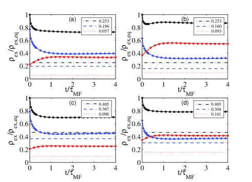
Figure 1: (Color online) Dynamics of the quantum depletion $\rho_{ex}(t)$ after the quench. The solid curves are the quantum depletion $\rho_{ex}(t)$ redistribution of a disordered Bose gas following a sudden change of interactions from $g_{i}$ to $g_{f}$ via the time. The dashed curves are the excitation fraction at the final interaction strength in equilibrium. The blue and red curves correspond to the interaction- and disordered-induced quantum depletion, whereas the black curve describes the quantum depletion due to the combined effects. The characteristic density and relaxation time are set by $\rho_{ex,eq}=1/3\pi^{2}\zeta^{3}+(1/4\pi\zeta^{3})\tilde{R}_{0}$ and $\tau_{MF}=\hbar/g_{f}\rho_{0}$ respectively. Parameters are given for (a) $\tilde{R}_{0}=0.1$ and $\tilde{g}=0.4$; (b) $\tilde{R}_{0}=0.2$ and $\tilde{g}=0.4$; (c) $\tilde{R}_{0}=0.1$ and $\tilde{g}=0.6$; (d) $\tilde{R}_{0}=0.2$ and $\tilde{g}=0.6$.

We shall focus on the regime of both weak interaction and weak disorder, in which Hamiltonian (1) can be well described using the standard Bogoliubov approximation Natu2013 ; Huang1992 ; YingHu2009 and the resulting expression reads

$$H_{\text{eff}}(t) = \sum_{\mathbf{k}\neq 0}\left(\epsilon_{\mathbf{k}}-\mu\right)\hat{a}_{\mathbf{k}}^{\dagger}\hat{a}_{\mathbf{k}}+\sqrt{\rho_{0}}\sum_{\mathbf{k}\neq 0}\left(\hat{a}_{\mathbf{k}}^{\dagger}V_{-\mathbf{k}}+\hat{a}_{\mathbf{k}}V_{\mathbf{k}}\right)$$ (4)

$$+ \frac{1}{2}g(t)\rho_{0}\sum_{\mathbf{k}\neq 0}\left(\hat{a}_{\mathbf{k}}^{\dagger}\hat{a}_{-\mathbf{k}}^{\dagger}+\hat{a}_{\mathbf{k}}\hat{a}_{-\mathbf{k}}\right),$$

where $\hat{a}_{\mathbf{k}}(\hat{a}_{\mathbf{k}}^{{\dagger}})$ annihilates (creates) a bosonic atom with momentum $\mathbf{k}$, and $\rho_{0}=N_{0}/V$ is the condensate density with $N_{0}$ being the number of condensed atoms. Hamiltonian (4) describes the process when a pair of bosonic atoms with momenta $\{\mathbf{k},-\mathbf{k}\}$ are annihilated through the two body interaction (and vice versa), as well as the process when a single particle with momenta $\mathbf{k}$ is scattered by the disordered potential into the condensate (and vice versa).

As the system is initially prepared at the ground state of Hamiltonian $H_{\text{eff}}$ (4) with $g=g_{i}$, the quench from $g_{i}$ to $g_{f}$ will bring the system to the nonequilibrium. For the quadratic Hamiltonian (4), the nonequilibrium dynamics can be exactly described as $|\Phi(t)\rangle=\Pi_{\mathbf{k}}U_{\mathbf{k}}(t)|\Phi(0)\rangle$ with $|\Phi(0)\rangle$ and $|\Phi(t)\rangle$ being the many-body wavefunction before and after the quench, respectively, and $U_{\mathbf{k}}\left(t\right)$ represents the evolution operator for each momenta $\mathbf{k}$. By noticing that Hamiltonian $H_{\text{eff}}$ with $g=g_{f}$ contains the operators of $K_{0}(\mathbf{k})=(\hat{a}_{\mathbf{k}}^{\dagger}\hat{a}_{\mathbf{k}}+\hat{a}_{-\mathbf{k}}^{\dagger}\hat{a}_{-\mathbf{k}})/2$, $K_{+}(\mathbf{k})=\hat{a}_{\mathbf{k}}^{\dagger}\hat{a}_{-\mathbf{k}}^{\dagger}$ and $K_{-}(\mathbf{k})=\hat{a}_{\mathbf{k}}\hat{a}_{-\mathbf{k}}$ which form the generators of SU(1,1) Lie algebra Quench1 ; Truax , we can obtain $U_{\mathbf{k}}(t)$ as

$$U_{\mathbf{k}}\left(t\right) = e^{\alpha_{\mathbf{k}}^{\ast}\left(t\right)\hat{a}_{\mathbf{k}}^{\dagger}}e^{\alpha_{\mathbf{k}}\left(t\right)\hat{a}_{\mathbf{k}}}\exp\left[\beta_{0}\left({\mathbf{k}},t\right)K_{0}\left(\mathbf{k}\right)+i\phi_{\mathbf{k}}\left(t\right)\right]$$ (5)

$$\times \exp\left[\beta_{+}\left(\mathbf{k},t\right)K_{+}\left(\mathbf{k}\right)\right]\exp\left[\beta_{-}\left(\mathbf{k},t\right)K_{-}\left(\mathbf{k}\right)\right].$$

Here, $\phi_{\mathbf{k}}(t)$ is a trivial phase and

$$\alpha_{\mathbf{k}}(t) = -\frac{\sqrt{\rho_{0}}}{\omega_{\mathbf{k}}}V_{\mathbf{k}}\left(\left|u_{\mathbf{k}}\right|^{2}+2u_{\mathbf{k}}v_{\mathbf{k}}^{\ast}+\left|v_{\mathbf{k}}\right|^{2}\right),$$

$$\beta_{+}(\mathbf{k},t) = v_{\mathbf{k}}^{\ast}(t)/u_{\mathbf{k}}^{\ast}(t),\beta_{-}(\mathbf{k},t)=-v_{\mathbf{k}}(t)/u_{\mathbf{k}}^{\ast}(t),$$

$$\beta_{0}(\mathbf{k},t) = -2\ln{u_{\mathbf{k}}^{\ast}(t)},$$ (6)

are expressed in terms of the disorder potential $V_{\mathbf{k}}$ and the time-dependent Bogoliubov amplitudes $u_{\mathbf{k}}(t)$ and $v_{\mathbf{k}}(t)$ which are determined from

$$\left(\begin{array}[]{c}u_{\mathbf{k}}(t)\\ v_{\mathbf{k}}(t)\end{array}\right) = \Bigg{[}\cos(\omega_{\mathbf{k}}^{f}t)\hat{I}-i\frac{\sin(\omega_{\mathbf{k}}^{f}t)}{\omega_{\mathbf{k}}^{f}}\times$$ (14)

$$\left(\begin{array}[]{cc}\epsilon_{\mathbf{k}}+g_{f}\rho_{0}&g_{f}\rho_{0}\\ -g_{f}\rho_{0}&-(\epsilon_{\mathbf{k}}+g_{f}n\rho_{0})\end{array}\right)\Bigg{]}\left(\begin{array}[]{c}u_{\mathbf{k}}\left(0\right)\\ v_{\mathbf{k}}\left(0\right)\end{array}\right),$$

with $u_{\mathbf{k}}\left(0\right)(v_{\mathbf{k}}\left(0\right))=\pm\sqrt{\left[(\epsilon_{\mathbf{k}}+\rho_{0}g_{i})/\omega_{\mathbf{k}}^{i}\pm 1\right]/2}$ and $\omega_{\mathbf{k}}^{f(i)}=\sqrt{\epsilon_{\mathbf{k}}\left(\epsilon_{\mathbf{k}}+2\rho_{0}g_{f(i)}\right)}$ and $\epsilon_{\mathbf{k}}=\hbar^{2}k^{2}/2m$. Note that $\left|u_{\mathbf{k}}\left(t\right)\right|^{2}-\left|v_{\mathbf{k}}\left(t\right)\right|^{2}=1$ is always satisfied during the time evolution. For self-consistency, hereafter we limit ourselves in the regime where the time dependence of $\rho_{0}$ can be ignored Natu2013 .

Quantum depletion after quench.– We are now well equipped to study the time evolution of the non-condensed fraction $\rho_{ex}(t)=\langle\Phi(0)|\sum_{\mathbf{k}}\hat{a}_{\mathbf{k}}^{\dagger}\hat{a}_{\mathbf{k}}|\Phi(0)\rangle$ of the considered system, given that the initial condition that $|\Phi(0)\rangle$ is the ground state of $H_{i}$. Straightforward derivation using Eq. (5) yields UedaBook

$$\rho_{ex}(t)=\sum_{\mathbf{k}}|\upsilon_{\mathbf{k}}(t)|^{2}.$$ (15)

By substituting Eq. (14) into Eq. (15), we can arrive at

$$\frac{\rho_{ex}(t)}{(3\pi^{2}\zeta^{3})^{-1}} = 1+\frac{3\pi\tilde{R}_{0}}{2+2\sqrt{\tilde{g}}}-3\sqrt{2}\int_{0}^{\infty}d{k}{\frac{\tilde{g}\left(1-\tilde{g}\right){k}^{2}\sin^{2}\left(\sqrt{{k}^{2}\left({k}^{2}+2\tilde{g}\right)}{t}\right)}{\left({k}^{2}+2\tilde{g}\right)\sqrt{{k}^{2}\left({k}^{2}+2\right)}}}$$ (16)

$$+ 6\sqrt{2}\tilde{R}_{0}\left(1-\tilde{g}\right)\int_{0}^{\infty}d{k}{\frac{2\left({k}^{4}+k^{2}+\tilde{g}k^{2}\right)\sin^{2}(\sqrt{{k}^{2}\left({k}^{2}+2\tilde{g}\right)}{t})+\tilde{g}(1-\tilde{g})\sin^{2}(2\sqrt{{k}^{2}\left({k}^{2}+2\tilde{g}\right)}{t})}{\left({k}^{2}+2\right)\left({k}^{2}+2\tilde{g}\right)^{3}}},$$

where $\zeta=\hbar/\sqrt{mg_{i}\rho_{0}}$ is the initial healing length, and we have introduced the dimensionless parameter

$$\tilde{R}_{0}=\rho_{0}R_{0}/(g_{i}\rho_{0})^{2}$$ (17)

to characterise the relative disorder strength. Note that, for vanishing disorder $\tilde{R}_{0}=0$, Equation (16) agrees exactly with the corresponding result in Ref. Natu2013 ; whereas for $\tilde{g}=1$ (no quench), the system simply remains in the ground state $|\Phi(0)\rangle$ with the depletion $\rho_{ex}=(3\pi^{2}\zeta^{3})\left[1+3\pi\tilde{R}_{0}/4\right]$ as in Ref. Huang1992 . Therefore, the last two terms in Eq. (16) presents the combined effect of the interaction quench $\tilde{g}\neq 1$ and disorder $\tilde{R}_{0}$ on the condensate depletion in the non-equilibrium regime.

We are interested in the asymptotic behavior of $\rho_{ex}(t)$ at the long time after the quench. To comprehensively reveal the roles of $\tilde{R}_{0}$ and $\tilde{g}$, we consider three cases for numerical analysis of Eq. (16), as illustrated in Fig. 1. (i) Firstly, we show how the quench strength $\tilde{g}$ affects the asymptotic depletion. As such, we fix $\tilde{R}_{0}=0$ and calculate $\rho_{ex}(t)$ (blue solid line), which is compared to the corresponding equilibrium depletion for a BEC with $g_{f}$ (blue dashed line). (ii) Secondly, to extract the role of disorder, we fix $\tilde{g}=0$ that corresponds to a quench to a non-interacting BEC (red solid line) with disorder, and then compare $\rho_{ex}(t)$ with the corresponding equilibrium value (red dashed line). (iii) Finally, the combined effects of disorder and quenched interaction is illustrated by the black solid curve. In all cases, we have found enhanced depletion in the asymptotic steady state compared to the corresponding case at zero temperature. This indicate that the ability of disorder or interaction to deplete the condensate is magnified in the non-equilibrium scenario.

Compared to the equilibrium disordered 3D BEC, the increased depletion in the steady state of the corresponding system under an interaction quench can be qualitatively understood in terms of the Loschmidt echo $L(t)=|\langle\Psi_{0}(t)|\Psi(t)\rangle|^{2}$ LE1 ; LE2 . The Loschmidt echo has been intensively studied recently in quenched systems. The connection between the condensate depletion and the Loschmidt echo is best illustrated in the case of $\tilde{R}=0$ in the quadratic Hamiltonian $H_{\text{eff}}$, when the Loschmidt echo can be calculated as $L(t)=1/\Pi_{\mathbf{k}}|u_{\mathbf{k}}|^{2}$ Quench1 . By using Eq. (15) and $|u_{\mathbf{k}}|^{2}=1+|\upsilon_{\mathbf{k}}|^{2}$, we estimate $L(t)\approx 1/(1+\rho_{ex}(t))$ (after ignoring higher order terms in $|u_{\mathbf{k}}|^{2}$ and $|\upsilon_{\mathbf{k}}|^{2}$ ). Then, building on the square relation $L_{sq}(t\rightarrow\infty)=L_{ad}^{2}(t\rightarrow\infty)$ established in Ref. Quench1 ; SQLE ; Heyl2013 , which connects the steady-state Loschmidt echo in a sudden quench ($L_{sq}$) to that of an adiabatic interaction change ($L_{ad}$), we can estimate $\rho_{ex}^{sq}(t\rightarrow\infty)=(1+\rho_{ex}^{ad})^{2}-1$. To see how this formula fits, we input the adiabatic value $\rho_{ex}^{eq}(t)/\rho_{ex,eq}=0.196$ (obtained from the dashed blue line in Fig. 1 a) and calculate the sudden quench depletion as $\rho_{ex}^{sq}(t\rightarrow\infty)/\rho_{ex,eq}=0.43$, which agrees fairly well with the numerical results in the steady state (solid blue line in Fig. 1 a).

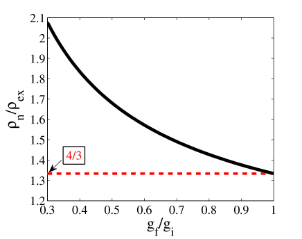
Figure 2: (Color online) Quench enhanced ratio between normal density $\rho_{n}$ in Eq. (19) and quantum depletion $\rho_{ex}(t\rightarrow\infty)$ in Eq. (16) via $g_{f}/g_{i}$. The dashed line corresponds to the value of $\rho_{n}/\rho_{ex}=4/3$ first obtained in Ref. Huang1992 .

Superfluid depletion after quench.– The superfluid component and the normal fluid component can be clearly distinguished from their response to a slow rotation: normal fluid rotates but superfluid does not. This is the essential concept behind typical experimental schemes to measure the superfluid density in an atomic Bose gas Cooper2010 ; Ho2009 ; Carusotto2011 . While the techniques to generate rotations in a Bose gas differ in various schemes, the key quantity measured boils down to the current-current response function $\chi_{i,j}\left(\mathbf{r}t,\mathbf{r}^{\prime}t^{\prime}\right)=\langle\left[J_{i}(\mathbf{r},t),J_{j}(\mathbf{r}^{\prime},t^{\prime})\right]\rangle$ ($i,j=x,y,z$) with $J_{i}\left(\mathbf{r},t\right)=\hbar/(2i)[\hat{\Psi}^{\dagger}(\mathbf{r})\nabla\hat{\Psi}(\mathbf{r})-\hat{\Psi}(\mathbf{r})\nabla\hat{\Psi}^{\dagger}(\mathbf{r})]$ being the current density of system and $\langle...\rangle$ averaged with the initial ground state $|\Psi(0)\rangle$. Particularly, the superfluid density $\rho_{s}$ corresponds to the response to the irrotational (longitudinal) part of the perturbation; whereas, the normal fluid density $\rho_{n}$ describes the transverse response, in an isotropic translationally invariant system, we have

$$m\chi_{ij}(\mathbf{q}\rightarrow 0,\omega)=\rho_{s}\frac{q_{i}q_{j}}{q^{2}}+\rho_{n}\delta_{ij}.$$ (18)

Based on the current experimental approaches to measure the superfluid response, we have calculated $\rho_{n}=\chi_{zz}(\mathbf{q}\rightarrow 0,\omega)$ with $J_{\mathbf{q}}^{z}=\hbar/(2m)\sum_{\mathbf{k}}(k_{z}+q_{z}/2)\hat{a}_{\mathbf{k}}^{\dagger}\hat{a}_{\mathbf{k+q}}$ for the steady state of the considered BEC after the interaction quench (as the system is isotropic, we are free to choose the slow rotation around the $z$ axis ). Then, by using Eqs. (5) and (14) UedaBook , we derive the normal fluid density in the steady state of the quenched system as

$$\frac{\rho_{n}}{(3\pi^{2}\zeta^{3})^{-1}} = \frac{2\pi\tilde{R}_{0}}{9\sqrt{\tilde{g}^{3}}}\Bigg{[}\left(7\tilde{g}-2\right)\frac{\mathtt{{}_{2}F_{1}}(\frac{1}{2},\frac{1}{2};1;\frac{(\tilde{g}-1)^{2}}{\tilde{g}^{2}})}{(\tilde{g}-1)/\tilde{g}}$$ (19)

$$- 5\frac{\mathtt{{}_{2}F_{1}}(-\frac{1}{2},\frac{1}{2};1;\frac{(\tilde{g}-1)^{2}}{\tilde{g}^{2}})}{(\tilde{g}-1)/\tilde{g}}\Bigg{]},$$

with $\mathtt{{}_{2}F_{1}(a,b;c;x)}$ being the hypergeometric function Mathematics .

Now, with both the condensate depletion and the normal fluid density at hand for the steady state of the considered system, we plot $\rho_{n}/\rho_{ex}$ as a function of the quench strength $\tilde{g}=g_{f}/g_{i}$, as illustrated in Fig. 2. To set a reference point, we have shown that in the limit $\tilde{g}\rightarrow 1$ (red dashed line), Eq. (19) exactly recovers the celebrated ratio $\rho_{n}/\rho_{ex}=4/3$ in Ref. Huang1992 for a ground-state BEC with weak disorder. In comparison, the quench effect (black solid line) gives rise to significantly enhanced ratio $\rho_{n}/\rho_{ex}$, the stronger the quench is, the higher value of $\rho_{n}/\rho_{ex}$ is found, which can even approach $2$. Moreover, we have found that the ratio does not depend on the individual absolute value of $g_{f}$ and $g_{i}$, but rather on their relative strength $\tilde{g}=g_{f}/g_{i}$. Figure 2 shows that the ability of disorder to deplete more superfluid than the condensate is remarkably amplified when combined with the quench effect, which presents the major result of this work. In principle, the value of $\rho_{s}/\rho_{0}$ can be further suppressed by repeating the process of sudden quench in the interaction: quench from $g_{i}$ to $g_{f}$, holding time $t$ and then adiabatically change interaction from $g_{f}$ to $g_{i}$, then quench interaction $n$ times (bang-bang protocol). It’s highly expected that the disordered BEC can be quenched into the regime of $\rho_{s}/\rho_{0}\ll 1$.

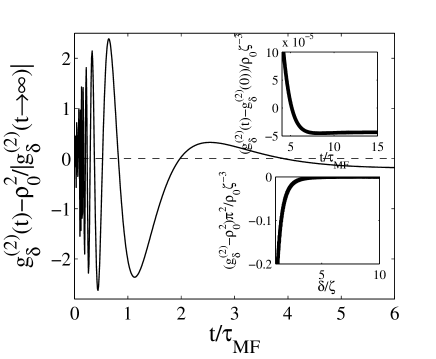
Figure 3: (Color online) Quench dynamics of density-density correlation function, which develops in an oscillatory manner and rapidly saturate at times $t-\delta/c>\tau_{MF}$ with $\delta$ being the separation between points, $\delta=|\mathbf{r}-\mathbf{r}^{{}^{\prime}}|$. The top inset: long-time density correlation function via time. The bottom inset: long-time behavior of density-density correlation function via the separation between points. The parameters are given as $\tilde{\delta}=\delta/\zeta=4$, $\tilde{g}=0.6$, and $\tilde{R}_{0}=0.1$.

Discussion and Conclusion.— We have shown that, by quenching in the interaction of a 3D BEC in disordered potential, the system can relax to a steady state where the ratio $\rho_{n}/\rho_{ex}>4/3$ can be achieved. This indicates the quench effect can significantly enhance the ability of disorder to deplete the superfluid more than the condensate, and therefore, suggests an alternative way of engineering Bose Glass in the dynamic regime. Central to testing our observation is the experimental ability to measure the condensate depletion $\rho_{ex}$ and normal fluid density $\rho_{n}$. In typical experiments, the-state-of-art higher-resolution imaging techniques allow one to probe the time-dependent quantum depletion $\rho_{ex}$ Xu ; Simon2011 ; Weitenberg2011 , while the experimental schemes reported in Refs. Cooper2010 ; Ho2009 ; Carusotto2011 can be used to measure $\rho_{n}$ in both equilibrium and nonequilibrium regimes. One concern that may arise is related to how fast the considered system can relax to the steady state. Figure 1 indicates the rapid relaxation of the one-body correlation. Let us further analyze the quench dynamics of the two-body correlation function, a quantity directly relevant for the the Bragg spectroscopy BraggOL1 ; BraggOL2 that has been a routine technique for studying excitations of a Bose gas. The two-body correlation function is defined as $g^{\left(2\right)}\left(t\right)=\sum_{\mathbf{q}}e^{i\mathbf{q}\cdot\left(\mathbf{r}-\mathbf{r}^{\prime}\right)}\left\langle\rho_{\mathbf{q}}\left(t\right)\rho_{-\mathbf{q}}\left(t\right)\right\rangle$ with $\rho_{\mathbf{q}}\left(t\right)=\sum_{\mathbf{k}}\hat{a}_{\mathbf{k}+\mathbf{q}}^{\dagger}\left(t\right)\hat{a}_{\mathbf{k}}\left(t\right)$ being the density operator. Following similar procedures Natu2013 , we calculate the correlation function from Eq. (5) and obtain

$$g_{\delta}^{\left(2\right)}\left(t\right) = \rho_{0}^{2}+\frac{\rho_{0}}{\pi^{2}\tilde{\delta}\zeta^{3}}\int kd{k}\sin\left(\sqrt{2}{k}\tilde{\delta}\right)\Big{[}\frac{k}{\sqrt{k^{2}+2}}-2\left(\tilde{g}-1\right)\frac{{k}\sin^{2}\left(\sqrt{{k}^{2}\left({k}^{2}+2\tilde{g}\right)}{t}\right)}{\sqrt{{k}^{2}+2}\left({k}^{2}+2\tilde{g}\right)}-1\Big{]}$$ (20)

$$+ \frac{4\rho_{0}}{\pi^{2}\tilde{\delta}\zeta^{3}}\tilde{R}_{0}\int d{k}\frac{{k}\sin\left(\sqrt{2}{k}\tilde{\delta}\right)}{\left({k}^{2}+2\right)\left({k}^{2}+2\tilde{g}\right)}\left\{\cos^{2}\left(\sqrt{{k}^{2}\left({k}^{2}+2\tilde{g}\right)}{t}\right)+\frac{{k}^{2}+2}{{k}^{2}+2\tilde{g}}\sin^{2}\left(\sqrt{{k}^{2}\left({k}^{2}+2\tilde{g}\right)}{t}\right)\right\}^{2},$$

with the dimensionless parameter $\tilde{\delta}=\delta/\zeta$ for $\delta=|\mathbf{r}-\mathbf{r}^{\prime}|$. Again, for vanishing disorder $\tilde{R}_{0}=0$, Equation (16) agrees with Ref. Natu2013 ; whereas for $\tilde{g}=1$, our result is consistent with Ref. Huang1992 . The time evolution of $g^{(2)}$ is presented in Fig. 3, which shows a rapid relaxation to a finite value on a time scale $t\sim 3\tau_{MF}$. Both the rapid relaxation of one-body matrix in Fig. 1 and the two-body correlation function in Fig. 3 suggest that, after the 3D disordered BEC is brought out of equilibrium by a quantum quench in the interaction, it relaxes to a steady state on a time-scale within the experimental reach.

We thank Biao Wu and Li You for stimulating discussions. This work is supported by the NSF of China (Grant Nos. 11004200 and 11274315). Y. H. also acknowledges support by the Austrian Science Fund (FWF) through SFB F40 FOQUS.

References

- (1) P. W. Anderson, Phys. Rev. 109, 1492 (1958).
- (2) J. A. Hertz, L. Fleishman, and P. W. Anderson, Phys. Rev. Lett. 43, 942 (1979); T. Giamarchi and H. J. Schulz, Phys. Rev. B 37, 325 (1988); K. G. Singh and D. S. Rokhsar, Phys. Rev. B 49, 9013 (1994); D. S. Fisher, and M. P. A. Fisher, Phys. Rev. Lett. 61, 1847 (1988); M. P. A. Fisher, P. B. Weichman, G. Grinstein, and D. S. Fisher, Phys. Rev. B 40, 546 (1989); D. K. K. Lee and J. M. F. Gunn, J. Phys. Condens. Matter 2, 7753 (1990); S. Giorini, L. Pitaevskii, and S. Stringari, Phys. Rev. B 49, 12938 (1994); M. Kobayashi and M. Tsubota, Phys. Rev. B 66, 174516 (2002).
- (3) I. Bloch, J. Dalibard, and W. Zwerger, Rev. Mod. Phys. 80, 885 (2008).
- (4) J. Billy, V. Josse, Z. Zuo, A. Bernard, B. Hambrecht, P. Lugan, D. Clément, L. Sanchez-Palencia, P. Bouyer and A. Aspect, Nature (London) 453, 891 (2011).
- (5) G. Roati, Chiara D’Errico, L. Fallani, M. Fattori, C. Fort, M. Zaccanti, G. Modugno, M. Modugno, and M. Inguscio, Nature (London) 453, 895 (2008).
- (6) L. Sanchez-Palencia and M. Lewenstein, Nat. Phys. 6, 87 (2010).
- (7) S. Krinner, D. Stadler, J. Meineke, J. P. Brantut, and T. Esslinger, Phys. Rev. Lett. 110, 100601 (2013).
- (8) M. Tavora, A. Rosch, and A. Mitra, Phys. Rev. Lett. 113, 010601 (2014).
- (9) C. D’Errico, E. Lucioni, L. Tanzi, L. Gori, G. Roux, and I. P. McCulloch, Phys. Rev. Lett. 113, 095301 (2014).
- (10) D. Pines and P. Noziéres, The theory of quantum liquids (Benjamin, New York, 1966), Vol. I; P. Noziéres and D. Pines, The theory of Quantum Liquids (Addison-Wesley, Reading, MA, 1990), Vol. II.
- (11) G. Baym, in Mathematical Methods in Solid State and Superfluid Theory, edited by R. C. Clark and G. H. Derrick (Oliver and Boyd, Edinburgh, 1969), p. 151.
- (12) L. P. Pitaevskii and S. Stringari, Bose-Einstein Condensation (Clarendon Press, Oxford, 2003).
- (13) K. Xu, Y. Liu, D. E. Miller, J. K. Chin, W. Setiawan, and W. Ketterle, Phys. Rev. Lett. 96, 180405 (2006).
- (14) N. R. Cooper and Z. Hadzibabic, Phys. Rev. Lett. 104, 030401 (2010); S. T. John, Z. Hadzibabic, and N. R. Cooper, Phys. Rev. A 83, 023610 (2011).
- (15) T. L. Ho and Q. Zhou, Nat. Phys. 6, 131 (2009).
- (16) I. Carusotto and Y. Castin, Phys. Rev. A 84, 053637 (2011).
- (17) J. Keeling, Phys. Rev. Lett. 107, 080402 (2011).
- (18) K. Huang and H. F. Meng, Phys. Rev. Lett. 69, 644 (1992).
- (19) A. V. Lopatin and V. M. Vinokur, Phys. Rev. Lett. 88, 235503 (2002).
- (20) G. E. Astrakharchik, J. Boronat, J. Casulleras, and S. Giorgini, Phys. Rev. A 66, 023603 (2002); N. Bilas and N. Pavloff, Eur. Phys. J. D 40, 387 (2006); M. Kobayashi and M. Tsubota, Phys. Rev. B 66, 174516 (2002). P. Lugan, D. Clément, P. Bouyer, A. Aspect, and L. Sanchez-Palencia, Phys. Rev. Lett. 99, 180402 (2007); G. M. Falco, A. Pelster, and R. Graham, Phys. Rev. A 75, 063619 (2007); L. Fontanesi, M. Wouters, and V. Savona, Phys. Rev. Lett. 103, 030403 (2009); J. Saliba, P. Lugan, and V. Savona, Phys. Rev. A Phys. Rev. A 90 031603 (2014).
- (21) V. I. Yukalov, Laser Phys. Lett. 1, 435 (2004); V. I. Yukalov, Ann. Phys. (N.Y.) 323, 461 (2008); V. I. Yukalov, E. P. Yukalova, K. V. Krutitsky, and R. Graham, Phys. Rev. A 76, 053623 (2007).
- (22) Y. Hu, Z. Liang, and B. Hu, Phys. Rev. A 80, 043629 (2009); Y. Hu, Z. Liang, and B. Hu, Phys. Rev. A 81 , 053621 (2010).
- (23) C. Gaul and C. A. Müller, Phys. Rev. A 83, 063629 (2011); P. Lugan and L. Sanchez-Palencia, Phys. Rev. A 84, 013612 (2011).
- (24) C. Chin, R. Grimm, P. Julienne and E. Tiesinga, Rev. Mod. Phys. 82, 1225 (2010).
- (25) S. S. Natu and E. J. Mueller, Phys. Rev. A 87, 053607 (2013).
- (26) B. Dóra, F. Pollmann, J. Fortágh, and G. Zaránd, Phys. Rev. Lett. 111, 040602 (2013).
- (27) D. R. Truax, Phys. Rev. D 31, 1988 (1985).
- (28) M. Ueda Fundamentals and new frontiers of Bose-Einstein Condensation, (World Scientific Publishing Co. Pte. Ltd. 2010).
- (29) A. Silva, Phys. Rev. Lett. 101, 120603 (2008)
- (30) R. Dorner, S. R. Clark, L. Heaney, R. Fazio, J. Goold, and V. Vedral, Phys. Rev. Lett. 110, 230601 (2013).
- (31) D. Rossini, T. Calarco, V. Giovannetti, S. Montangero, and R. Fazio, Phys. Rev. A 75, 032333 (2007).
- (32) M. Heyl, A. Polkovnikov, and S. Kehrein, Phys. Rev. Lett. 110, 135704 (2013).
- (33) D. Zwillinger, Standard Mathematical Tables and Formulae (CRC Press, 2011).
- (34) J. Simon, W. S. Bakr, R. Ma, M. E. Tai, P. M. Preiss, and M. Greiner, Nature (London) 472, 307 (2011).
- (35) C. Weitenberg, M. Endres, J. F. Sherson, M. Cheneau, P. Schauß, T. Fukuhara, I. Bloch, and S. Kuhr, Nature (London) 471, 319 (2011).
- (36) P. T. Ernst, S. Götze, J. S. Krauser, K. Pyka, D. S. Lühmann, D. Pfannkuche and K. Sengstock, Nat. Phys. 6, 56 (2010).
- (37) X. Du, S. Wan, E. Yesilada, C. Ryu, D. J. Heinzen Z. X. Liang and B. Wu, New. J. Phys. 12, 083025 (2010).