Shortcuts to adiabatic passage for multiqubit controlled phase gate

Abstract

Abstract: We propose an alternative scheme of shortcuts to quantum phase gate in a much shorter time based on the approach of Lewis-Riesenfeld invariants in cavity quantum electronic dynamics (QED) systems. This scheme can be used to perform one-qubit phase gate, two-qubit controlled phase gate and also multiqubit controlled phase gate. The strict numerical simulation for some quantum gates are given, and demonstrate that the total operation time of our scheme is shorter than previous schemes and very robustness against decoherence.
Keywords: Shortcuts to adiabatic passage $\cdot$ one-qubit phase gate $\cdot$ multiqubit controlled phase gate

I Introduction

It is well known that quantum gates play a significant role in quantum computing, and any quantum gate operation can be decomposed into a series of one-qubit gates and two-qubit conditional gates, such as one-qubit phase gate, and two-qubit controlled-NOT gate DPD1995 ; AB1995 . Recently, a number of schemes have been proposed to perform quantum logic gates using optical devices YFH2004 , QED system SBZ2013 , quantum dotBQH2002 , ion trap and superconducting devices JIC1995 ; M2001 ; CPY2003 ; CPY2006 . Moreover, the implementations of two-qubit conditional gates in experiment have been proposed MAN2000 ; SLB2001 . However, the controlled phase gates with more than three qubits is difficult in experimental implementation. Even though a $N$-qubit controlled phase gate could be decomposed into one- and two-qubit gates, it would be extremely complex for a practical problem, even worse, it would increase the total operation time so that the decoherence arising which will destroy the quantum system eventually. Recently, a great many schemes have been proposed to perform quantum logical gate via adiabatic passage HGK2004 ; ZKF2002 ; BRS2013 ; DDB2014 . For example, Hayato Goto et al. implemented the multiqubit controlled unitary gate by adiabatic passage with an optical cavityHGK2004 . Zheng implemented a $\pi$ phase gate through the adiabatic evolution SBZ2005 . Rydberg-interaction gates with adiabatic passage was proposed in DDB2014 . All these schemes are based on adiabatic passage technique, because this method allows the initial state evolve along the dark state to the target state accurately.

However, the adiabatic condition usually requires a relatively long interaction time and then slows down the speed of the system evolution, and finally the dissipation caused by decoherence, noise, and losses would destroy the expected dynamics. Therefore, accelerating the dynamics towards the target outcome would be the most reasonable and effective way to actually fight against the decoherence. Thus, the shortcuts to adiabatic passage for various reliable, fast, and robust schemes have been drawn a lot of attentions in both theory and experiment ARXD2012 ; XASA2010 ; KPYR2011 ; AC2013 ; MYLJ2014 ; YYQJ2014 ; AFTS2012 ; JXPP2011 . However the shortcuts to logical gates have not been fully studied. Chen et al. YHC2014 proposed a scheme of shortcuts to performing a $\pi$ phase gate through designing the particular resonant laser pulses by the invariant-based inverse engineering. It was the only scheme for quantum logic gates based on shortcuts to adiabatic passage in cavity QED systems.

In this paper, we construct an effective shortcuts to adiabatic passage to perform one-qubit phase gate, two-qubit controlled phase gate, three-qubit controlled phase gate and also multiqubit controlled phase gate based on the Lewis-Riesenfeld invariants and quantum Zeno dynamics. The logical gates in our scheme can be performed in a much shorter time than that based on adiabatic passage technique. Moreover, this scheme is insensitive to the decoherence caused by spontaneous emission and photon leakage which is demonstrated by the strict numerical simulation.

This paper is structured as follows: In Sec. II, we give a brief description about Lewis-Riesenfeld invariants. In Sec. III, we construct a shortcuts to one-qubit phase gate. Two-qubit controlled phase gate, three-qubit controlled phase gate and multiqubit controlled phase gate are presented in Sec. IV. In Sec. V we give the numerical simulation and feasibility analysis for our schemes. The conclusion appears in Sec. VI.

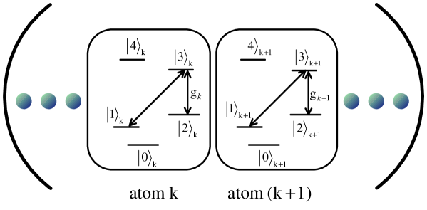
Figure 1: The schematic setup for multiqubit phase gate. The $N$ five levels atoms which have the same level structure are trapped in a single mode optical cavity.

II Lewis-Riesenfeld invariants

We first give a brief description about Lewis-Riesenfeld invariants theory HRL1969 ; MAL2009 . A quantum system is governed by a time-dependent Hamiltonian $H(t)$, and the corresponding time-dependent Hermitian invariant $I(t)$ satisfies

$$i\hbar\frac{\partial I(t)}{\partial t} = [H(t),I(t)].$$ (1)

The solution of the time-dependent Schrödinger equation $i\hbar$ $\frac{\partial|\Psi(t)\rangle}{\partial t}$ $=H(t)|\Psi(t)\rangle$ can be expressed by a superposition of invariant $I(t)$ dynamical modes $|\Phi_{n}(t)\rangle$:

$$|\Psi(t)\rangle = \sum_{n}C_{n}e^{i\alpha_{n}}|\Phi_{n}(t)\rangle,$$ (2)

where $C_{n}$ is a time-independent amplitude, $\alpha_{n}$ is the Lewis-Riesenfeld phase, $|\Phi_{n}(t)\rangle$ are orthonormal eigenvectors of the invariant $I(t)$, satisfying $I(t)|\Phi_{n}(t)\rangle=\lambda_{n}|\Phi_{n}(t)\rangle$, with $\lambda_{n}$ real constants. And the Lewis-Riesenfeld phases are defined as

$$\alpha_{n}(t) = \frac{1}{\hbar}\int_{0}^{\prime}dt^{\prime}\langle\Phi_{n}(t^{\prime})|i\hbar\frac{\partial}{\partial t^{\prime}}-H(t^{\prime})|\Phi_{n}(t^{\prime})\rangle.$$ (3)

III Shortcuts to adiabatic passage for one-qubit phase gate

The schematic setup for our scheme is shown in Fig. 1, $N$ identical five-level atoms trapped in a single mode optical cavity. Every atom possesses three ground states $|0\rangle$, $|1\rangle$, $|2\rangle$ and two excited states $|3\rangle$, $|4\rangle$. The state $|2\rangle$ and $|3\rangle$ is strongly coupled with the cavity mode field, and the other transitions $|1\rangle\rightarrow|4\rangle$, $|2\rangle\rightarrow|4\rangle$, $|1\rangle\rightarrow|3\rangle$, $|0\rangle\rightarrow|3\rangle$ are resonant with the classical laser field.

We now consider the one-qubit $\pi$ phase gate. In this case, only one qubit is trapped in the single mode optical cavity. Choosing the initial state of the qubit is $|\Psi_{0}\rangle=\alpha|0\rangle+\beta|1\rangle$, after performing the $\pi$ phase gate, the outcome state becomes:

$$|\Psi\rangle=\alpha|0\rangle-\beta|1\rangle.$$ (4)

In the following, we explain the detail of how to construct the shortcuts to adiabatic passage for one-qubit $\pi$ phase gate. We choose the laser pulses resonant with the transition $|1\rangle\rightarrow|4\rangle$ and $|2\rangle\rightarrow|4\rangle$ transitions, and the corresponding Rabi frequencies are denoted by $\Omega_{1}(t)$ and $\Omega_{2}(t)$, respectively. The interaction Hamiltonian in the interaction picture is given by ($\hbar=1$)

$$H(t)=\Omega_{1}(t)|4\rangle\langle 1|+\Omega_{2}(t)|4\rangle\langle 2|+\rm H.c.$$ (5)

To speed up the gate performing by the dynamics of invariant based inverse engineering, we need to find out the Hermitian invariant operator $I(t)$, which satisfies $i\hbar\frac{\partial I(t)}{\partial t}=[H(t),I(t)]$, and here $H(t)$ possesses SU(2) dynamical symmetry, so $I(t)$ can be easily given by XCE2011

$$I(t)=\chi\left(\cos\gamma\sin\beta|4\rangle\langle 1|+\cos\gamma\cos\beta|4\rangle\langle 2|+i\sin\gamma|2\rangle\langle 1|\right),$$ (6)

$\chi$ is an arbitrary constant with units of frequency to keep $I(t)$ with dimensions of energy, $\gamma$, and $\beta$ are time-dependent auxilary parameters which satisfy the equations

$$\dot{\gamma} = \Omega_{1}(t)\cos\beta-\Omega_{2}(t)\sin\beta,$$

$$\dot{\beta} = \tan\gamma(\Omega_{2}(t)\cos\beta+\Omega_{1}(t)\sin\beta).$$ (7)

From Eq. (7) we can derive the expressions of $\Omega_{1}(t)$ and $\Omega_{2}(t)$ as follow:

$$\Omega_{1}(t) = \dot{\beta}\cot\gamma\sin\beta+\dot{\gamma}\cos\beta,$$

$$\Omega_{2}(t) = \dot{\beta}\cot\gamma\cos\beta-\dot{\gamma}\sin\beta.$$ (8)

The eigenstates of the invariant $I(t)$ are

$$|\Phi_{0}(t)\rangle = \cos\gamma\cos\beta|1\rangle-i\sin\gamma|4\rangle-\cos\gamma\sin\beta|2\rangle,$$

$$|\Phi_{\pm}(t)\rangle = \frac{1}{\sqrt{2}}[(\sin\gamma\cos\beta\pm i\sin\beta)|1\rangle+i\cos\gamma|4\rangle-(\sin\gamma\sin\beta\mp i\cos\beta)|2\rangle].$$ (9)

The solution of the Schrödinger equation $i\hbar$ $\frac{\partial|\Psi(t)\rangle}{\partial t}$ $=H(t)|\Psi(t)\rangle$ can be written with the eigenstates of $I(t)$ as

$$|\Psi(t)\rangle = \sum_{n=0,\pm}C_{n}e^{i\alpha_{n}}|\Phi_{n}(t)\rangle,$$ (10)

where $\alpha_{n}(t)$ are the Lewis-Riesenfeld phases presented in Eq. (3), and in this case, $C_{n}=\langle\Phi_{n}(0)|1\rangle$.

In order to generate a $\pi$ phase on the state $|1\rangle$, we choose the parameters as

$$\gamma(t) = \epsilon,~{}~{}~{}~{}~{}~{}~{}~{}~{}\beta(t)=\pi t/t_{f},$$ (11)

with $\epsilon$ is a time-independent small value and $t_{f}$ is the total operation time. Then, we obtain

$$\Omega_{1}(t) = \frac{\pi}{t_{f}}\cot\epsilon\sin\frac{\pi t}{t_{f}},$$

$$\Omega_{2}(t) = \frac{\pi}{t_{f}}\cot\epsilon\cos\frac{\pi t}{t_{f}}.$$ (12)

When $t=t_{f}$,

$$|\Psi(t_{f})\rangle = (-\cos^{2}\epsilon-\sin^{2}\epsilon\cos\alpha)|1\rangle+(-i\sin\epsilon\cos\epsilon+i\sin\epsilon\cos\epsilon\cos\alpha)|4\rangle$$ (14)

$$-\sin\epsilon\sin\alpha|2\rangle,$$

where $\alpha=\pi/\sin\epsilon=|\alpha_{\pm}|$. When we choose $\alpha=2N\pi(N=1,2,3...)$, $|\Psi(t_{f})\rangle=-|1\rangle$. On the other hand, the state $|0\rangle$ does not participate in the evolvtion. Therefore, the $\pi$ phase gate can be achieved

$$|\Psi_{0}\rangle=\alpha|0\rangle+\beta|1\rangle\rightarrow|\Psi\rangle=\alpha|0\rangle-\beta|1\rangle.$$ (15)

IV Shortcuts to adiabatic passage for controlled phase gate

IV.1 Two-qubit controlled $\pi$ phase gate

In this section, a two-qubit controlled $\pi$ phase gate is proposed. We consider two identical five-level atoms trapped in a single mode optical cavity as shown in Fig. 1. The initial state of two atoms is defined as

$$|\Psi_{0}\rangle=\alpha_{00}|00\rangle+\alpha_{01}|01\rangle+\alpha_{10}|10\rangle+\alpha_{11}|11\rangle,$$ (16)

where $\alpha_{ij}(i,j=0,1)$ denote the probability amplitude of the state $|ij\rangle$. After performing the controlled $\pi$ phase gate, the output is

$$|\Psi\rangle=\alpha_{00}|00\rangle+\alpha_{01}|01\rangle+\alpha_{10}|10\rangle-\alpha_{11}|11\rangle,$$ (17)

where the first atom is control qubit, and the second atom acts as target qubit. In order to construct the shortcuts to adiabatic passage for two-qubit controlled $\pi$ phase gate, there are mainly three steps.

Step 1: The second atom state $|1\rangle_{2}$ is transferred to $-|2\rangle_{2}$ by the shortcuts with laser pulses resonant with $|1\rangle_{2}\rightarrow|4\rangle_{2}$ and $|2\rangle_{2}\rightarrow|4\rangle_{2}$, and the corresponding Rabi frequencies are denoted by $\Omega_{1}(t)$ and $\Omega_{2}(t)$. Using the similar method mentioned in Sec. III, and the only difference is that we choose $\gamma(t)=\epsilon$ and $\beta(t)=\frac{\pi t}{2t_{f}}$, then obtain

$$\Omega_{1}(t) = \frac{\pi}{2t_{f}}\cot\epsilon\sin\frac{\pi t}{2t_{f}},$$

$$\Omega_{2}(t) = \frac{\pi}{2t_{f}}\cot\epsilon\cos\frac{\pi t}{2t_{f}}.$$ (18)

When $t=t_{f}$ and $\alpha=2N\pi(N=1,2,3...)$ , the transition $|1\rangle_{2}\rightarrow-|2\rangle_{2}$ can be achieved. Then the initial state $|\Psi_{0}\rangle$ becomes

$$|\Psi_{1}\rangle=\alpha_{00}|00\rangle-\alpha_{01}|02\rangle+\alpha_{10}|10\rangle-\alpha_{11}|12\rangle.$$ (19)

Step 2: The state $|12\rangle$ generates a $\pi$ phase by the shortcuts and then becomes $-|12\rangle$ with laser pulses resonant with the first atom $|1\rangle_{1}\rightarrow|3\rangle_{1}$ and the second atom $|1\rangle_{2}\rightarrow|3\rangle_{2}$, and the corresponding Rabi frequencies denoted by $\Omega^{(1)}(t)$ and $\Omega^{(2)}(t)$. By means of shortcuts, the state $|\Psi_{1}\rangle$ becomes

$$|\Psi_{2}\rangle=\alpha_{00}|00\rangle-\alpha_{01}|02\rangle+\alpha_{10}|10\rangle+\alpha_{11}|12\rangle.$$ (20)

The detail of this step will be explained later.

Step 3: The same with step 1, the second atom state $|2\rangle_{2}$ is transferred back to $-|1\rangle_{2}$ by the shortcuts with laser pulses resonant with $|2\rangle_{2}\rightarrow|4\rangle_{2}$ and $|1\rangle_{2}\rightarrow|4\rangle_{2}$, and the corresponding Rabi frequencies are denoted by $\Omega_{2}(t)=\frac{\pi}{2t_{f}}\cot\epsilon\sin\frac{\pi t}{2t_{f}}$and $\Omega_{1}(t)=\frac{\pi}{2t_{f}}\cot\epsilon\cos\frac{\pi t}{2t_{f}}$, when $t=t_{f}$ and $\alpha=2N\pi(N=1,2,3...)$, we can obtain

$$|\Psi_{3}\rangle=\alpha_{00}|00\rangle+\alpha_{01}|01\rangle+\alpha_{10}|10\rangle-\alpha_{11}|11\rangle.$$ (21)

Thus, the two-qubit controlled $\pi$ phase gate can be achieved.

In the following, we explain how to realize step 2 in detail. We have choose the laser pulses resonant with the first atom $|1\rangle_{1}\rightarrow|3\rangle_{1}$ transition and the second atom $|1\rangle_{2}\rightarrow|3\rangle_{2}$ transition with the corresponding Rabi frequencies denoted by $\Omega^{(1)}(t)$ and $\Omega^{(2)}(t)$. The Hamiltonian for this step is given by

$$H(t)=\Omega^{(1)}(t)|3\rangle_{1}\langle 1|+\Omega^{(2)}(t)|3\rangle_{2}\langle 1|+g_{1}a_{1}|3\rangle_{1}\langle 2|+g_{2}a_{2}|3\rangle_{2}\langle 2|+\rm H.c,$$ (22)

where $g_{1,2}$ are the coupling constants between atoms and cavity field modes, and $a_{1,2}$ are the annihilation operators of photons. We choose $g_{1}=g_{2}$ and $a_{1}=a_{2}$ for simplicity. In this case, if the system is in $|12\rangle_{1,2}|0\rangle_{c}$, the evolution subspace can be spanned by

$$|\varphi_{1}\rangle = |12\rangle_{1,2}|0\rangle_{c},~{}~{}~{}|\varphi_{2}\rangle=|32\rangle_{1,2}|0\rangle_{c},~{}~{}~{}|\varphi_{3}\rangle=|22\rangle_{1,2}|1\rangle_{c},$$

$$|\varphi_{4}\rangle = |23\rangle_{1,2}|0\rangle_{c},~{}~{}~{}|\varphi_{5}\rangle=|21\rangle_{1,2}|0\rangle_{c},$$ (23)

where $|0\rangle_{c}$ and $|1\rangle_{c}$ denote the photon number state in the cavity field. With the help of quantum Zeno dynamics, the effective Hamiltonian is given by YYQJ2014

$$H_{eff}(t)=\frac{1}{\sqrt{2}}|\mu\rangle(\Omega^{(1)}(t)\langle\varphi_{1}|+\Omega^{(2)}(t)\langle\varphi_{5}|+\rm{H.c)},$$ (24)

where $|\mu\rangle=\frac{1}{\sqrt{2}}(-|\varphi_{2}\rangle+|\varphi_{4}\rangle)$. It is obvious that the effective Hamiltonian $H_{eff}(t)$ possesses the SU(2) dynamical symmetriy, too. Thus, we can use the same method presented in Sec. III. Choosing $\gamma=\epsilon$ and $t_{f}=\frac{\pi t}{t_{f}}$, thus, $\Omega^{(1)}(t)=\frac{\pi}{t_{f}}\cot\epsilon\sin\frac{\pi t}{t_{f}}$ and $\Omega^{(2)}(t)=\frac{\pi}{t_{f}}\cot\epsilon\cos\frac{\pi t}{t_{f}}$. When $t=t_{f}$, $|12\rangle\rightarrow-|12\rangle$ can be achieved.

If the initial state of the system is $|10\rangle_{1,2}|0\rangle_{c}$, the vectors of the system evolution subspace are given by

$$|\phi_{1}\rangle = |10\rangle_{1,2}|0\rangle_{c},~{}~{}~{}|\phi_{2}\rangle=|30\rangle_{1,2}|0\rangle_{c},~{}~{}~{}|\phi_{3}\rangle=|20\rangle_{1,2}|1\rangle_{c}.$$ (25)

For this case, the initial state $|10\rangle_{1,2}|0\rangle_{c}$ evolves along the dark state

$$|\phi_{dark}\rangle=g|\phi_{1}\rangle-\Omega^{(1)}(t)|\phi_{3}\rangle.$$ (26)

With the parameters above, when $t=t_{f}$, $\Omega^{(1)}(t)=0$, and then $|\phi_{dark}\rangle=|\phi_{1}\rangle$. It is obvious that the state $|00\rangle$ and $|02\rangle$ do not change any more in this step. Thus the state in Eq. (19) can be obtained.

IV.2 Three-qubit controlled $\pi$ phase gate

The three-qubit controlled $\pi$ phase gate can be described as follow: The three atoms initial state is given by

$$|\Psi_{0}\rangle=\sum_{l_{1},l_{2},l_{3}=0,1}\alpha_{l_{1}l_{2}l_{3}}|l_{1}l_{2}l_{3}\rangle,$$ (27)

where $\alpha_{l_{1}l_{2}l_{3}}$ denote the probability amplitude of the three five-level atoms state $|l_{1}l_{2}l_{3}\rangle(l_{1},l_{2},l_{3}=0,1)$. After performing the controlled $\pi$ phase gate, the output becomes

$$|\Psi\rangle=\sum_{l_{1},l_{2},l_{3}=0,1}e^{il_{1}l_{2}l_{3}\pi}\alpha_{l_{1}l_{2}l_{3}}|l_{1}l_{2}l_{3}\rangle,$$ (28)

with atom 1 and atom 2 are the two control qubits and atom 3 is the target qubit. In order to construct the shortcuts to adiabatic passage for three-qubit controlled $\pi$ phase gate, there are mainly four steps.

Step 1: The third atom state $|1\rangle_{3}$ is transferred to $-|2\rangle_{3}$ by the shortcuts with laser pulses resonant with $|1\rangle_{3}\rightarrow|4\rangle_{3}$ and $|2\rangle_{3}\rightarrow|4\rangle_{3}$ transitions, and the corresponding Rabi frequencies are denoted by $\Omega_{1}(t)$ and $\Omega_{2}(t)$. Similar to the method mentioned in the step 1 of two-qubit controlled $\pi$ phase gate, we also choose $\gamma(t)=\epsilon$ and $\beta(t)=\frac{\pi t}{2t_{f}}$, when $t=t_{f}$ we can obtain

$$|\Psi_{1}\rangle=\sum_{l_{1},l_{2}=0,1}(\alpha_{l_{1}l_{2}0}|l_{1}l_{2}0\rangle-\alpha_{l_{1}l_{2}1}|l_{1}l_{2}2\rangle).$$ (29)

Step 2: The state $|l_{1}12\rangle$ is transferred to $-|l_{1}21\rangle$ with laser pulses resonant with the second atom $|1\rangle_{2}\rightarrow|3\rangle_{2}$ transition and the third atom $|1\rangle_{3}\rightarrow|3\rangle_{3}$ transition with the corresponding Rabi frequencies are denoted by $\Omega^{(2)}(t)$ and $\Omega^{(3)}(t)$. Then, the state $|\Psi_{1}\rangle$ becomes

$$|\Psi_{2}\rangle=\sum_{l_{1},l_{2}=0,1}(\alpha_{l_{1}l_{2}0}|l_{1}l_{2}0\rangle-\alpha_{l_{1}01}|l_{1}02\rangle+\alpha_{l_{1}11}|l_{1}21\rangle).$$ (30)

The detail of this step will be explained later.

Step 3: The state $|021\rangle$ transferred to $-|021\rangle$ with laser pulses resonant with the first atom $|0\rangle_{1}\rightarrow|3\rangle_{1}$ transition and the second atom $|0\rangle_{2}\rightarrow|3\rangle_{2}$ transition, and the corresponding Rabi frequencies denoted by $\Omega^{\prime(1)}(t)$ and $\Omega^{\prime(2)}(t)$. Then, the state $|\Psi_{2}\rangle$ becomes

$$|\Psi_{3}\rangle=\sum_{l_{1},l_{2}=0,1}\alpha_{l_{1}l_{2}0}|l_{1}l_{2}0\rangle-\sum_{l_{1}=0,1}\alpha_{l_{1}01}|l_{1}02\rangle-\alpha_{011}|021\rangle+\alpha_{111}|121\rangle.$$ (31)

The detail of this step will be explained later, too.

Step 4: $|2\rangle_{2(3)}$ is back to $-|1\rangle_{2(3)}$ by the shortcuts with the similar method to step 1. As a result, the output is

$$|\Psi_{4}\rangle = \sum_{l_{1},l_{2}=0,1}\alpha_{l_{1}l_{2}0}|l_{1}l_{2}0\rangle+\sum_{l_{1}=0,1}\alpha_{l_{1}01}|l_{1}01\rangle+\alpha_{011}|011\rangle-\alpha_{111}|111\rangle$$ (33)

$$=\sum_{l_{1},l_{2},l_{3}=0,1}e^{il_{1}l_{2}l_{3}\pi}\alpha_{l_{1}l_{2}l_{3}}|l_{1}l_{2}l_{3}\rangle.$$

Thus, the three-qubit controlled $\pi$ phase gate can be realized.

In the following, we explain the step 2 in detail. We have choose the laser pulses resonant with the second atom $|1\rangle_{2}\rightarrow|3\rangle_{2}$ transition and the third atom $|1\rangle_{3}\rightarrow|3\rangle_{3}$ transition, and the corresponding Rabi frequencies denoted by $\Omega^{(2)}(t)$ and $\Omega^{(3)}(t)$. The Hamiltonian is given by

$$H(t)=\Omega^{(2)}(t)|3\rangle_{2}\langle 1|+\Omega^{(3)}(t)|3\rangle_{3}\langle 1|+g_{2}a_{2}|3\rangle_{2}\langle 2|+g_{3}a_{3}|3\rangle_{3}\langle 2|+\rm H.c,$$ (34)

where $g_{2,3}$ are the coupling constants between atoms and cavity field modes, and $a_{2,3}$ are the annihilation operators of photons. We choose $g_{2}=g_{3}$ and $a_{2}=a_{3}$ for simplicity. In this case, if the second and the third atoms state is $|12\rangle_{2,3}$ , the evolution subspace spanned by

$$|\varphi_{1}\rangle = |12\rangle_{2,3}|0\rangle_{c},~{}~{}~{}|\varphi_{2}\rangle=|32\rangle_{2,3}|0\rangle_{c},~{}~{}~{}|\varphi_{3}\rangle=|22\rangle_{2,3}|1\rangle_{c},$$

$$|\varphi_{4}\rangle = |23\rangle_{2,3}|0\rangle_{c},~{}~{}~{}|\varphi_{5}\rangle=|21\rangle_{2,3}|0\rangle_{c}.$$ (35)

where $|0\rangle_{c}$ and $|1\rangle_{c}$ denote the photon number state in the cavity field. The same with step 2 in the section of two-qubit controlled $\pi$ phase gate, we now choose the parameter $\gamma(t)=\epsilon$, $\beta(t)=\frac{\pi t}{2tf}$ and $\alpha=2N\pi$, when $t=t_{f}$, we can obtain $-|\varphi_{5}\rangle$, and this step is successful. On the other hand, the other states will not change in this step.

And then, we explain the step 3 in detail. In this step, we choose the laser pulses resonant with the first atom $|0\rangle_{1}\rightarrow|3\rangle_{1}$ transition and the second atom $|0\rangle_{2}\rightarrow|3\rangle_{2}$ transition, and the corresponding Rabi frequencies are denoted by $\Omega^{\prime(1)}(t)$ and $\Omega^{\prime(2)}(t)$. The Hamiltonian is given by

$$H(t)=\Omega^{\prime(1)}(t)|3\rangle_{1}\langle 0|+\Omega^{\prime(2)}(t)|3\rangle_{2}\langle 0|+g^{\prime}_{1}a^{\prime}_{1}|3\rangle_{1}\langle 2|+g^{\prime}_{2}a^{\prime}_{2}|3\rangle_{3}\langle 2|+H.c,$$ (36)

where $g_{1^{\prime},2^{\prime}}$ are the coupling constants between atoms and cavity field modes, and $a_{1^{\prime},2^{\prime}}$ are the annihilation operators of photons. We choose $g_{1^{\prime}}=g_{2^{\prime}}$ and $a_{1^{\prime}}=a_{2^{\prime}}$ for simplicity. The vectors in this step are

$$|\xi_{1}\rangle = |02\rangle_{1,2}|0\rangle_{c},~{}~{}~{}|\xi_{2}\rangle=|32\rangle_{1,2}|0\rangle_{c},~{}~{}~{}|\xi_{3}\rangle=|22\rangle_{1,2}|1\rangle_{c},$$

$$|\xi_{4}\rangle = |23\rangle_{1,2}|0\rangle_{c},~{}~{}~{}|\xi_{5}\rangle=|20\rangle_{1,2}|0\rangle_{c}.$$ (37)

The same with the method described in step 2 in the section of two-qubit controlled $\pi$ phase gate, we now choose the parameter $\gamma(t)=\epsilon$, $\beta(t)=\frac{\pi t}{tf}$ and $\alpha=2N\pi$, when $t=t_{f}$, we can obtain $-|02\rangle_{1,2}$, and the other states will not change in this step.

IV.3 Multiqubit controlled $\pi$ phase gate

We consider $n+1$ atoms are trapped in a single mode cavity as shown in Fig. 1. In general, $(n+1)$-qubit controlled $\pi$ phase gate can be described as follow: The $(n+1)$ atoms is in the initial state

$$|\Psi_{0}\rangle=\sum_{l_{1},l_{2}...l_{n+1}=0,1}\alpha_{l_{1}l_{2}...l_{n+1}}|l_{1}l_{2}...l_{n+1}\rangle.$$ (38)

After performing the $(n+1)$-qubit controlled $\pi$ phase gate, we can obtain

$$|\Psi\rangle=\sum_{l_{1},l_{2}...l_{n+1}=0,1}e^{i\pi l_{1}l_{2}...l_{n+1}}\alpha_{l_{1}l_{2}...l_{n+1}}|l_{1}l_{2}...l_{n+1}\rangle.$$ (39)

Here, the first $n$ qubits are the control qubits, and the last qubit is target qubit. In order to construct the shortcuts to $(n+1)$-qubit controlled $\pi$ phase gate, there are four steps.

Step 1: $|1\rangle_{n+1}$ is transferred to $-|2\rangle_{n+1}$ by the laser pulses resonant with the $(n+1)th$ atom $|1\rangle_{n+1}\rightarrow|4\rangle_{n+1}$ and $|2\rangle_{n+1}\rightarrow|4\rangle_{n+1}$ transitions. Then the initial state becomes

$$|\Psi_{1}\rangle=\sum_{l_{1},l_{2}...l_{n}=0,1}(\alpha_{l_{1}l_{2}...l_{n}0}|l_{1}l_{2}...l_{n}0\rangle-\alpha_{l_{1}l_{2}...l_{n}1}|l_{1}l_{2}...l_{n}2\rangle).$$ (40)

Step 2: The state $|l_{1}l_{2}...l_{n-1}12\rangle$ transferred to $-|l_{1}l_{2}...l_{n-1}21\rangle$ with laser pulses resonant with the $nth$ atom $|1\rangle_{n}\rightarrow|3\rangle_{n}$ transition and the $(n+1)th$ atom $|1\rangle_{n+1}\rightarrow|3\rangle_{n+1}$ transition, and the corresponding Rabi frequencies denoted by $\Omega^{(n)}(t)$ and $\Omega^{(n+1)}(t)$. Then, the state $|\Psi_{1}\rangle$ becomes

$$|\Psi_{2}\rangle = \sum_{l_{1},l_{2}...l_{n}=0,1}\alpha_{l_{1}l_{2}...l_{n}0}|l_{1}l_{2}...l_{n}0\rangle-\sum_{l_{1},l_{2}...l_{n-1}=0,1}\alpha_{l_{1}l_{2}...l_{n-1}01}|l_{1}l_{2}...l_{n-1}02\rangle$$ (42)

$$+\sum_{l_{1},l_{2}...l_{n-1}=0,1}\alpha_{l_{1}l_{2}...l_{n-1}11}|l_{1}l_{2}...l_{n-1}21\rangle.$$

Step 3: The state $|l_{1}l_{2}...l_{n-1}21\rangle$ transferred to $-|l_{1}l_{2}...l_{n-1}21\rangle$, here $l_{1},l_{2}...l_{n-1}$ satisfied the condition $l_{1}\cdot l_{2}\cdot...\cdot l_{n-1}=0$. Choosing the laser pulses resonant with the $kth$ atom $|0\rangle_{k}\rightarrow|3\rangle_{k}$ $(k=1,2...n-1)$ transition and the $nth$ atom $|0\rangle_{n}\rightarrow|3\rangle_{n}$ transition, and the corresponding Rabi frequencies denoted by $\Omega^{\prime(k)}(t)$ and $\Omega^{\prime(n)}(t)$. Then, the state $|\Psi_{2}\rangle$ becomes

$$|\Psi_{3}\rangle = \sum_{l_{1},l_{2}...l_{n}=0,1}\alpha_{l_{1}l_{2}...l_{n}0}|l_{1}l_{2}...l_{n}0\rangle-\sum_{l_{1},l_{2}...l_{n-1}=0,1}\alpha_{l_{1}l_{2}...l_{n-1}01}|l_{1}l_{2}...l_{n-1}02\rangle$$ (44)

$$-\sum_{l_{1},l_{2}...l_{n-1}=0,1}\alpha_{l_{1}l_{2}...l_{n-1}11}|l_{1}l_{2}...l_{n-1}21\rangle_{(l_{1}\cdot l_{2}\cdot...l_{n-1}=0)}+\alpha_{11...1}|1...21\rangle.$$

Step 4: $|2\rangle_{n(n+1)}$ is back to $-|1\rangle_{n(n+1)}$ by the shortcuts. As a result, the output is

$$|\Psi_{4}\rangle = \sum_{l_{1},l_{2}...l_{n}=0,1}\alpha_{l_{1}l_{2}...l_{n}0}|l_{1}l_{2}...l_{n}0\rangle+\sum_{l_{1},l_{2}...l_{n-1}=0,1}\alpha_{l_{1}l_{2}...l_{n-1}01}|l_{1}l_{2}...l_{n-1}01\rangle$$ (47)

$$+\sum_{l_{1},l_{2}...l_{n-1}=0,1}\alpha_{l_{1}l_{2}...l_{n-1}11}|l_{1}l_{2}...l_{n-1}11\rangle_{(l_{1}\cdot l_{2}\cdot...l_{n-1}=0)}-\alpha_{11...1}|1...11\rangle$$

$$=\sum_{l_{1},l_{2}...l_{n+1}=0,1}e^{i\pi l_{1}l_{2}...l_{n+1}}\alpha_{l_{1}l_{2}...l_{n+1}}|l_{1}l_{2}...l_{n+1}\rangle.$$

That is a $(n+1)$-qubit controlled $\pi$ phase gate.

V Numerical simulations and feasibility analysis

In this section, we make the numerical simulations for one-qubit $\pi$ phase gate and two-qubit controlled $\pi$ phase gate by numerically solving the Schr$\ddot{\rm o}$dinger equations. We also discuss the influence of spontaneous emission and decay of cavity on fidelity.

V.1 One-qubit $\pi$ phase gate

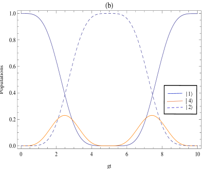
Figure 2: (a) Time dependence of $\Omega_{1(2)}(t)/g$ of the laser fields for performing one-qubit $\pi$ phase gate. (b) Time evolutions of the populations of corresponding system states. Here, the system parameters are set to be $\epsilon=0.25$ and $t_{f}=10/g.$

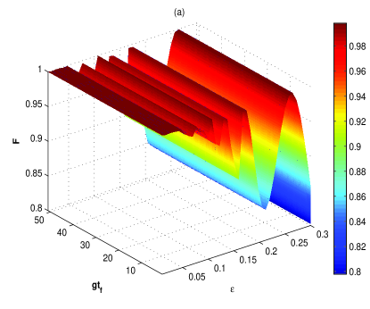
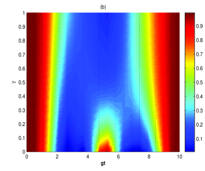
Figure 3: (a) The fidelity of one-qubit $\pi$ phase gate versus $\epsilon$ and $t_{f}$ regardless of the atom decay. (b) The fidelity of one-qubit $\pi$ phase gate versus the evolution time $t$ and the spontaneous emission rate $\gamma$ of atom. The system parameters are set to be $\epsilon=0.25$ and $t_{f}=10/g.$

We consider the initial state of the single atom is given by:

$$|\Psi_{0}\rangle=\frac{1}{\sqrt{2}}(|0\rangle+|1\rangle).$$ (48)

Fig. 2(a) shows the scaled Rabi frequencies $\Omega_{1}(t)/g$ and $\Omega_{2}(t)/g$ versus $gt$ when $\epsilon=0.25$ and $gt_{f}=10$, where $\Omega_{1}(t)$ and $\Omega_{2}(t)$ is defined in Eq. (12). The population curves of $|1\rangle$, $|4\rangle$ and $|2\rangle$ versus $gt$ are depicted in Fig. 2(b). From Fig. 2(b) we can see a perfect population transfer from the initial state $|1\rangle$ and then back to $|1\rangle$ after the whole involution, and generate a $\pi$ phase which can be known from Eq. (13). Through the above processes, we construct the shortcuts for one-qubit $\pi$ phase gate successfully. As expected, the final state is

$$|\Psi\rangle=\frac{1}{\sqrt{2}}(|0\rangle-|1\rangle).$$ (49)

Fig. 3(a) shows the fidelity $F(t_{f})=\langle-1|\Psi(t_{f})$ as a function of $\epsilon$ and $gt_{f}$ when the initial state is $|1\rangle$. Fig. 3(a) demonstrates that, the effect of $t_{f}$ on fidelity can be ignored. In our scheme, we choose $\epsilon=0.25$, and the fidelity can be higher than $99\%$.

Next, we investigate the influence of spontaneous emission of atom on the gate fidelity. The evolution of the system is governed by the master equation

$$\dot{\rho} = i[\rho,H]+\sum_{i=1,2}\frac{\gamma}{2}[|i\rangle\langle 4|\rho|4\rangle\langle i|-\frac{1}{2}(|4\rangle\langle 4|\rho+\rho|4\rangle\langle 4|)],$$ (50)

$\gamma$ is the spontaneous emission rate of atom. We plot the fidelity $F(t)=|\langle-1|\rho(t)|-1\rangle|$ as a function of the operation time $t$ and spontaneous emission rate $\gamma$ in Fig. 3(b), with $\rho(t)$ being density matrix at $t$ and $|-1\rangle$ being the target state, and the other parameters are $\epsilon=0.25$ and pulse duration $t_{f}=10/g$. The evolutions are governed by the Hamiltonian defined in Eq. (5). From Fig. 3(b) we can see that, when the total evolution time $t=t_{f}$, the fidelity of our scheme can be higher than $99.7\%$, in other words, our scheme is insensitive to the spontaneous emission of atom.

V.2 two-qubit $\pi$ phase gate

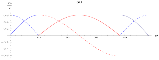
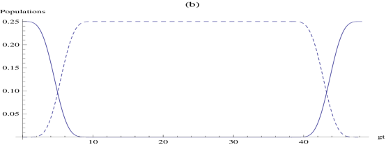
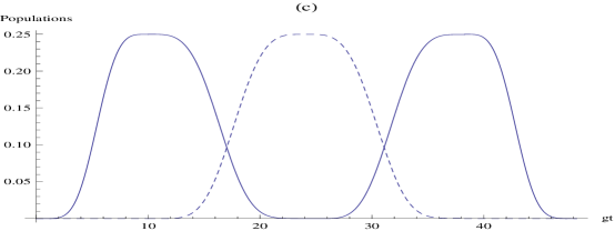
Figure 4: (a) Time dependence of $\Omega_{i}(t)/g$ of the laser fields for two-qubit controlled $\pi$ phase gate with $\Omega_{i}(t)=\Omega_{1}(t)$ (solid blue line), $\Omega_{2}(t)$ (dash blue line), $\Omega^{(1)}(t)$ (solid red line), $\Omega^{(2)}(t)$ (dash red line). (b) Time evolutions of the populations of corresponding system states $|01\rangle$ (solid blue line) and $-|02\rangle$ (dash blue line). (c) Time evolutions of the populations of corresponding system states $|12\rangle$ (solid blue line) and $|21\rangle$ (dash blue line). The system parameters are set to be $\epsilon=0.25$ and $t_{f}=10/g.$

We consider the initial state of the two atom is given by:

$$|\Psi_{0}\rangle=\frac{1}{2}(|00\rangle+|01\rangle+|10\rangle+|11\rangle).$$ (51)

The coupling rate of atom and cavity field mode are chosen as $g_{1}=g_{2}=g$. We depict the scaled Rabi frequencies $\Omega_{1}(t)/g$, $\Omega_{2}(t)/g$ ,$\Omega^{(1)}(t)/g$ and $\Omega^{(2)}(t)/g$ versus $gt$ in Fig. 4(a), and the other parameters are chosen as $\epsilon=0.25$ and $gt_{f}=10$, where $\Omega_{1}(t)$ and $\Omega_{2}(t)$ is defined in Eq. (17), $\Omega^{(1)}(t)$ and $\Omega^{(2)}(t)$ are the same form with Eq. (12). The population curves of $|01\rangle$ (solid blue line) and $|02\rangle$ (dash blue line) versus $gt$ are shown in Fig. 4(b). Fig. 4(c) shows the population of $|12\rangle$ (solid blue line) and $|21\rangle$ (dash blue line) versus $gt$.  Through the above processes, we construct the shortcuts to two-qubit $\pi$ phase gate successfully. As expected, the final state is

$$|\Psi\rangle=\frac{1}{2}(|00\rangle+|01\rangle+|10\rangle-|11\rangle).$$ (52)

We note that, in the step 2 of two-qubit controlled $\pi$ phase gate, the vectors including $|\varphi_{3}\rangle=|22\rangle_{2,3}|1\rangle_{c}$ in Eq. (33), i.e. there is a photon in the cavity. Therefore, we must both investigate the influence of cavity decay and spontaneous emission on the gate fidelity. The evolution of the system is governed by the master equation

$$\dot{\rho} = i[\rho,H]+\sum_{k=1}^{5}[L_{k}\rho L_{k}^{+}-\frac{1}{2}(L_{k}^{+}L_{k}\rho+\rho L_{k}^{+}L_{k})],$$ (53)

where $L_{k}$ and $L_{k}^{+}$ are the Lindblad operators MJK2011 , and they have the following form

$$L_{1} = \sqrt{\kappa}a,~{}~{}~{}~{}~{}~{}~{}~{}~{}~{}~{}~{}~{}~{}~{}L_{2}=\sqrt{\gamma_{1}}|1\rangle_{2}\langle 3|,~{}~{}~{}~{}~{}~{}~{}L_{3}=\sqrt{\gamma_{2}}|1\rangle_{3}\langle 3|,$$

$$L_{4} = \sqrt{\gamma_{3}}|2\rangle_{2}\langle 3|,~{}~{}~{}~{}~{}~{}~{}L_{3}=\sqrt{\gamma_{4}}|2\rangle_{3}\langle 3|,$$ (54)

where $\kappa$ is the decay rate of cavity and $\gamma_{i}(i=1,2,3,4)$ are the corresponding spontaneous emission rates of atoms, and $H$ is defined by Eq. (32). We choose $\gamma_{i}=\gamma$. We plot the fidelity $F(t)=|\langle-12|\rho(t)|-12\rangle|$ as a function of the operation time $t$ and cavity decay rate $\kappa$ in Fig. 5(a)), and as a function of the operation time $t$ and spontaneous emission rate $\gamma$ in Fig. 5(b)), with $\rho(t)$ being density matrix at $t$ and $|-12\rangle$ being the target state, and the other parameters are $\epsilon=0.25$ and pulse duration $t_{f}=20\sqrt{2}/g$. From Fig. 5(a) and Fig. (b) we can see that, when the total evolution time $t=t_{f}$, the fidelity of our scheme is closed to 1. Therefore, our scheme is robust against the cavity decay and spontaneous emission, and must be feasible in experiment.

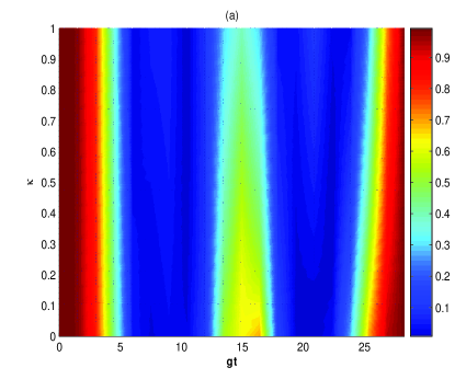
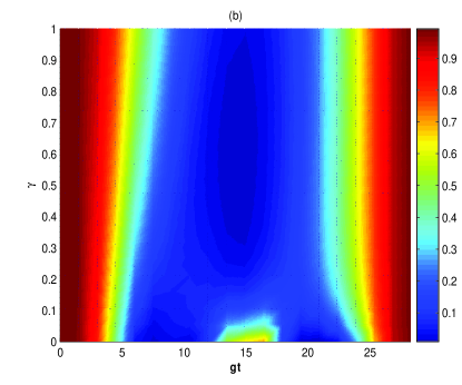
Figure 5: (a) The fidelity of the step 2 of two-qubit controlled $\pi$ phase gate versus $\kappa$ and the evolution time $t$. (b) The fidelity of the step 2 of two-qubit controlled $\pi$ phase gate versus the spontaneous emission of atom $\gamma$ and the evolution time $t$. The system parameters are set to be $\epsilon=0.25$ and $t_{f}=20\sqrt{2}/g.$

We now analyze the feasibility in experiment for this scheme. The appropriate atomic level configuration can be realized with trapped ions and cavity QED systems SSD2000 ; JPH2002 ; LYX2003 or with impurity levels in a solid, such as Pr³⁺ ions in Y₂SiO₅ crystal KI2001 , or nitrogen-vacancy color center in diamond MSS2002 . In experiments, the cavity QED parameters $(g,\kappa,\gamma)/2\pi=(750,3.5,2.62)$ MHz is predicted to be available in an optical cavity SMS2005 . In our scheme, when the cavity decay rate and the spontaneous emission rate is comparable to atom cavity coupling constant $g$, the fidelity is also higher than $99\%$. Thus, our scheme is robust against both the cavity decay and atomic spontaneous radiation and may be very promising within current experiment technology.

VI Conlusion

In summary, we have proposed a promising scheme to construct shortcuts to perform one-qubit phase gate and muliqubit controlled phase gate by invariant-based inverse engineering. Compared with the previous work, the interaction time required for the gate operation is much shorter than that with the method of adiabatic passage. The shortcuts to our scheme is not only fast, but also robust against the decoherence caused by atomic spontaneous emission and cavity decay, so it can be a more reliable choice in experiment.

$\mathbf{ACKNOWLEDGMENTS}$

This work was supported by the National Natural Science Foundation of China under Grant Nos. 11464046 and 61465013.

References

- (1) DiVincenzo, D. P.: Two-bit gates are universal for quantum computation. Phys. Rev. A 51, 1015 (1995).
- (2) Barenco, A., Bennett, C. H., Cleve, R., DiVincenzo, D. P., Margolus, N., Shor, P., Sleator, T., Smolin, J., Weinfurter, H.: Elementary gates for quantum computation. Phys. Rev. A 52, 3457 (1995).
- (3) Huang, Y. F., Ren, X. F., Zhang, Y. S., Duan, L. M., Guo, G. C.: Experimental teleportation of a quantum controlled-NOT gate. Phys. Rev. Lett. 93, 240501 (2004).
- (4) Zheng, S. B.: Implementation of toffoli gates with a single asymmetric Heisenberg XY interaction. Phys. Rev. A 87, 042318 (2013).
- (5) Qiao, B., Ruda, H. E., Wang, J.: Multiqubit computing and error-avoiding codes in subspace using quantum dots. J. Appl. Phys. 91, 2524 (2002).
- (6) Cirac, J. I., Zoller, P.: Quantum Computations with Cold Trapped Ions. Phys. Rev. Lett. 74, 4091 (1995).
- (7) aura, M., Buek, V.: Multiparticle entanglement with quantum logic networks: Application to cold trapped ions. Phys. Rev. A 64, 012305 (2001).
- (8) Yang, C. P., Chun, S.: Possible realization of entanglement, logical gates, and quantum-information transfer with superconducting-quantum-interference-device qubits in cavity QED. Phys. Rev. A 67, 042311 (2003).
- (9) Yang, C. P., Han, S.: Realization of an n-qubit controlled-U gate with superconducting quantum interference devices or atoms in cavity QED. Phys. Rev. A 73, 032317 (2006).
- (10) Nielsen, M. A., Chuang, I. L.: Quantum Computation and Quantum Information. (Cambridge University Press, Cambridge, 2000).
- (11) DiVincenzo, D. P., Braunstein, S. L., Lo, H. K.: Scalable Quantum Computers (Wiley- VCH, Berlin, 2001).
- (12) Goto, H., Ichimura, K.: Multiqubit controlled unitary gate by adiabatic passage with an optical cavity. Phys. Rev. A 70, 012305 (2004).
- (13) Kis, Z., Renzoni, F.: Qubit rotation by stimulated Raman adiabatic passage. Phys. Rev. A 65, 032318 (2002).
- (14) Roussraux, B., Guérin, S., Vitanov, N. V.: Arbitrary qudit gates by adiabatic passage. Phys. Rev. A 87, 032328(2013).
- (15) Rao, D. D. B., Mlmer, K.: Robust Rydberg-interaction gates with adiabatic passage. Phys. Rev. A 89, 030301(R) (2014).
- (16) Zheng, S. B.: Nongeometric conditional phase shift via adiabatic evolution of dark eigenstates: a new approach to quantum computation. Phys. Rev. Lett. 95, 080502 (2005).
- (17) Ruschhaupt, A., Chen, X., Alonso, D., Muga, J. G.: Optimally robust shortcuts to population inversion in two-level quantum systems. New J. Phys. 14, 093040 (2012).
- (18) Chen, X., Lizuain, I., Ruschhaupt, A., Guéry-Odelin, D., Muga, J. G.: shortcut to adiabatic passage in two- and three-level atoms. Phys. Rev. Lett. 105, 123003 (2010).
- (19) Hoffmann, K. H., Salamon, P., Rezek, Y., Kosloff, R.: Time-optimal controls for frictionless cooling in harmonic traps. Euro. Phys. Lett. 96, 60015 (2011).
- (20) del Campo, A.: Shortcuts to adiabaticity by counter-diabatic driving. Phys. Rev. Lett. 111, 100502 (2013).
- (21) Lu, M., Xia, Y., Shen, L. T., Song, J., An, N. B.: Shortcuts to adiabatic passage for population transfer and maximum entanglement creation between two atoms in a cavity. Phys. Rev. A 89, 012326 (2014).
- (22) Chen, Y. H., Xia, Y., Chen, Q. Q., Song, J.: Efficient shortcuts to adiabatic passage for fast population transfer in multiparticle systems. Phys. Rev. A 89, 033856 (2014).
- (23) Walther, A., Ziesel, F., Ruster, T., Dawkins, S. T., Ott, K., Hettrich, M., Singer, K., Schmidt-Kaler, F., Poschinger, U.: Controlling fast transport of cold trapped ions. Phys. Rev. Lett. 109, 080501 (2012).
- (24) Schaff, J. F., Song, X. L., Capuzzi, P., Vignolo, P., Labeyrie, G.: Shortcut to adiabaticity for an interacting Bose-Einstein condensate. Euro. Phys. Lett. 93, 23001 (2011).
- (25) Cheng, Y. H., Xia, Y., Chen, Q. Q., Song, J.: Fast and noise-resistant implementation of quantum phase gates and creation of quantum entangled states. arXiv preprint arXiv: 1410, 8285 (2014).
- (26) Lewis, H. R., Riesenfeld, W. B.: An exact quantum theory of the timeDependent harmonic oscillator and of a charged particle in a timeDependent electromagnetic field. J. Math. Phys. 10, 1458 (1969).
- (27) Lohe, M. A.: Exact time dependence of solutions to the time-dependent Schr odinger equation. J. Phys. A: Math. and Theor. 42, 035307 (2009).
- (28) Chen, X., Torrontegui, E., Muga, J. G.: Lewis-Riesenfeld invariants and transitionless quantum driving. Phys. Rev. A 83, 062116 (2011).
- (29) Kastoryano, M. J., Reiter, F., Sørensen, A. S.: Dissipative preparation of entanglement in optical cavities. Phys. Rev. Lett. 106, 090502 (2011).
- (30) Schneider, S., James, D., Milburn, G. J.: Quantum computation with hot trapped ions. J. Mod. Opt. 47, 499 (2000).
- (31) Pachos, J., Walther, H.: Quantum computation with trapped ions in an optical cavity. Phys. Rev. Lett. 89, 187903 (2002).
- (32) You, L., Yi, X. X., Su, X. H.: Quantum logic between atoms inside a high-Q optical cavity. Phys. Rev. A 67, 032308 (2003).
- (33) Ichimura, K.: A simple frequency-domain quantum computer with ions in a crystal coupled to a cavity mode. Opt. Commun. 196, 119 (2001).
- (34) Shahriar, M. S., Hemmer, P. R., Lloyd, S., Bhatia, P. S., Craig, A. E.: Solid-state quantum computing using spectral holes. Phys. Rev. A 66, 032301 (2002).
- (35) Spillane, S. M., Kippenberg, T. J., Vahala, K. J., Goh, K. W., Wilcut, E., Kimble, H. J.: Ultrahigh-Q toroidal microresonators for cavity quantum electrodynamics. Phys. Rev. A 71, 013817 (2005).