Spitzer Secondary Eclipses of the Dense, Modestly-irradiated, Giant Exoplanet HAT-P-20b Using Pixel-Level Decorrelation

Abstract

HAT-P-20b is a giant metal-rich exoplanet orbiting a metal-rich star. We analyze two secondary eclipses of the planet in each of the 3.6- and 4.5 $\mu$m bands of Warm Spitzer. We have developed a simple, powerful, and radically different method to correct the intra-pixel effect for Warm Spitzer data, which we call pixel-level decorrelation (PLD). PLD corrects the intra-pixel effect very effectively, but without explicitly using - or even measuring - the fluctuations in the apparent position of the stellar image. We illustrate and validate PLD using synthetic and real data, and comparing the results to previous analyses. PLD can significantly reduce or eliminate red noise in Spitzer secondary eclipse photometry, even for eclipses that have proven to be intractable using other methods. Our successful PLD analysis of four HAT-P-20b eclipses shows a best-fit blackbody temperature of $1134\pm 29$K, indicating inefficient longitudinal transfer of heat, but lacking evidence for strong molecular absorption. We find sufficient evidence for variability in the 4.5 $\mu$m band that the eclipses should be monitored at that wavelength by Spitzer, and this planet should be a high priority for JWST spectroscopy. All four eclipses occur about 35 minutes after orbital phase $0.5$, indicating a slightly eccentric orbit. A joint fit of the eclipse and transit times with extant RV data yields $e\cos{\omega}=0.01352^{+0.00054}_{-0.00057}$, and establishes the small eccentricity of the orbit to high statistical confidence. HAT-P-20b is another excellent candidate for orbital evolution via Kozai migration or other three-body mechanism.

1 Introduction

The transiting exoplanet HAT-P-20b occupies a unique niche in parameter space, being a massive ($M=7.246\pm 0.187\,M_{J}$), high density planet ($\rho=13.8\pm 1.5\,g\,cm^{-3}$), orbiting a relatively small metal-rich star ($R=0.69\pm 0.02R_{\odot},[Fe/H]=+0.35\pm 0.08$ Bakos et al., 2011). The high metallicity of the star, and the radius of the massive planet being smaller than Jupiter ($R_{p}=0.867\pm 0.033R_{J}$, Bakos et al., 2011), suggest that the planet is metal-rich. Moreover, HAT-P-20b is only moderately irradiated, with a predicted equilibrium temperature of 970K (for zero albedo and uniform longitudinal distribution of heat).

Spitzer observations of exoplanets like HAT-P-20b, with equilibrium temperatures below 1000K, are targets of a new Spitzer program (H. Knutson, P.I.) to search for a plausible inverse relation between planetary mass and atmospheric metallicity. That relation should be especially obvious at temperatures where methane forms ($\lessapprox 1000$K), because methane abundance can be supressed by CO formation when the atmospheric metallicity is very high (Moses et al., 2013). We therefore anticipate the possibility of strong molecular absorption, due to either methane or CO, in cool giant exoplanets like HAT-P-20b. Indeed, Spitzer eclipses of the moderately irradiated exo-Neptune GJ 436b are interpreted as exhibiting strong CO absorption, and a large depletion of methane (Stevenson et al., 2010; Lanotte et al., 2014).

Although we seek the molecular absorption spectra of giant transiting planets, it has been argued that the emergent spectra of some hot Jupiters - such as the strongly-irradiated WASP-12b - are consistent with that of a blackbody (Crossfield et al., 2012). However, Stevenson et al. (2014) concludes that the spectrum of WASP-12b deviates decisively from a blackbody. Recently, Hansen et al. (2014) have suggested that the dayside spectra of all close-in giant transiting planets are adequately described as blackbodies, based on their inferred level of systematic error in the Spitzer analyses. Irrespective of this debate, there are already multiple examples in the literature where the emergent dayside spectra of hot Jupiters are consistent with that of a blackbody. For example, Corot-1b (Deming et al., 2011), WASP-48b and HAT-P-23b (O’Rourke et al., 2014) resemble blackbodies. However, there are also planets whose emergent spectrum is clearly not a blackbody, WASP-43b being the most recent example (Kreidberg et al., 2014).

Our observations of HAT-P-20b have two motivations. First, we want to detect molecular absorption or emission in the non-blackbody spectrum of a moderately-irradiated metal-rich giant exoplanet. Second, we aspire to improve techniques for hot Jupiter photometry, by reducing the level of systematic error in Warm Spitzer analyses. To that end, we have developed a simple, powerful, and radically different new methodology for producing high quality photometry from Spitzer images at 3.6 and 4.5 $\mu$m. In this paper, we report a two-point photometric ‘spectrum’ of HAT-P-20b, based on two eclipses observed in each Warm Spitzer band, and we discuss the implications for the atmosphere and orbit of the planet.

This paper is organized as follows. In Sec. 2, we introduce our new pixel-level decorrelation (PLD) technique for analyses of Spitzer data, and we argue for its advantages over traditional methods. Sec. 3 explains how we implement PLD in practice, and Sec. 4 validates it by applying it to synthetic data where the underlying transit, eclipse, and phase curve amplitudes are known. Sec. 5 describes application of PLD to real data for several exoplanetary systems previously analyzed using traditional methods, and we compare our PLD results and error levels to those previous analyses. Having thus validated PLD as an effective tool for Spitzer analyses, we apply it to HAT-P-20b. Sec. 6 describes our new observations, and the initial processing of the data. Sec. 7 derives the PLD eclipse amplitudes of HAT-P-20b, and Secs. 8 and 9 discuss the implications of our results for the atmosphere and orbit of HAT-P-20b, respectively. Sec. 10 summarizes our conclusions.

2 The Zen of Intra-pixel Decorrelation

We here motivate and describe our new PLD technique, which differs fundamentally from all other methods used to analyze Spitzer data to date.

Photometry of IRAC images at 3.6 and 4.5 $\mu$m has long been known (Charbonneau et al., 2005) to exhibit a systematic effect due to intra-pixel sensitivity variations (Ingalls et al., 2012). When coupled with pointing jitter, the intra-pixel sensitivity variations produce intensity fluctuations that must be removed from photometry in order to detect the subtle eclipses of exoplanets. Current methods to correct Spitzer photometry are based on defining and removing a correlation between apparent intensity fluctuations of the host star, and its physical position on the detector as determined by finding the centroid of the stellar PSF. The earliest such decorrelations (e.g., Charbonneau et al., 2005; Knutson et al., 2008; Machalek et al., 2008) modeled the intensity fluctuations as polynomial (typically quadratic) functions of the Y-coordinate, sometimes with a weaker (e.g., linear) dependence on the X-coordinate. Polynomial decorrelations are still used (e.g., Shporer et al., 2014), but methods have evolved to include very powerful implementations such as Bi-Linear Interpolated Sub-pixel Sensitivity (BLISS) mapping (Stevenson et al., 2012), and novel variants such as a spatial weighting-function approach (Ballard et al., 2010; Cowan et al., 2012), and modifications thereof (Lewis et al., 2013; Zellem et al., 2014; Lanotte et al., 2014). These decorrelations have been largely, but not entirely successful. Their success is illustrated by very precise observations such as the transits of GJ1214b (Fraine et al., 2013; Gillon et al., 2014). However, their limitation is indicated by residual red noise that is often found, especially in the 3.6 $\mu$m band where the intra-pixel effect is strongest.

All current methods to remove Spitzer’s intra-pixel effect rely on defining a relationship between photometric fluctuations and the position of the stellar image on the detector. However, PLD neither defines nor requires any functional relation between intensity fluctuations and the position of the stellar image. Although we determine the position of the stellar image in order to measure its intensity within a circular aperture (i.e., do photometry), we do not use the image position per se to correct the intensity fluctuations. We assert a zen-like irony: the best way to correct the effect of fluctuations in image position does not involve using the position of the image.

We point out that the position of the stellar image is a secondary data product, derived from the intensities registered by the pixels of the detector. The intensities of individual pixels are the primary data. Conventional methods use the pixel intensities to define an image position via a numerical process (e.g., determining center-of-light or fitting a 2-D Gaussian). The centroid position of the star is then related to intensity fluctuations by a second numerical process (e.g., BLISS mapping, or polynomial fits). In defining the position-intensity relation, the star is implicitly treated as a point source, when in fact it has a width comparable to the pixels it is traversing. PLD omits these two intermediate numerical steps, and relates the fluctuations in total intensity to the individual pixels directly, using a simple, physically-motivated, linear expression, as we now describe.

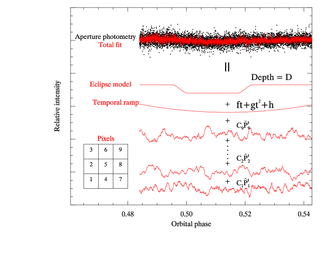
For most Spitzer secondary eclipse observations, the star moves by less than one pixel over the entire time series. Positional stability of Spitzer images has been greatly facilitated by reductions in pointing jitter (Grillmair et al., 2012), and reproducibility of target acquisition (Ingalls et al., 2012). A relatively few pixels typically encapsulate most of the information concerning the total brightness and position of the stellar image. As the image moves (for example) in the +Y direction, the pixel immediately above the centroid receives a greater proportion of the total flux, and the pixel immediately below the centroid receives less of the total flux. The position of the image is thus encoded in the relative intensities of the pixels. Hence, PLD uses positional information implicitly, but not explicitly. We consider a small group of pixels that contain the stellar image, typically a $3\times 3$-pixel square approximately centered on the star. Indexing the 2-dimensional grid of $N$ pixels using a single index, let the background-subtracted intensity of pixel $i$ at time $t$ be denoted $P_{i}^{t}$. The measured brightness of the star, $S^{t}$, in a frame of data at time $t$ can be written as:

$$S^{t}={\mathcal{F}}(P_{1}^{t},P_{2}^{t},P_{3}^{t},...P_{N}^{t}),$$ (1)

where $\mathcal{F}$ is a generalized function. Because the PSF of the telescope is broader than an individual pixel, $S^{t}$ varies smoothly with the position of the image. In that physical situation, $\mathcal{F}$ is continuous and differentiable, and we can apply a Taylor series expansion to derive an expression for the fluctuations in $S^{t}$ as a function of the changes in $P_{i}^{t}$. For small fluctuations in image position, we can approximate the Taylor expansion using only the linear terms:

$$\delta S^{t}=\sum_{i=1}^{N}\frac{\partial{\mathcal{F}}}{\partial{P}_{i}^{t}}{\delta{P}_{i}^{t},}$$ (2)

where the lower case $\delta$ indicates the fluctuations in $S^{t}$ caused only by the combination of image motion and spatial inhomogeneities of the detector. To utilize Eq. (2) in actual data analysis, we first normalize the pixel intensities so that their sum is unity at each time step, thus:

$$\hat{P}_{i}^{t}=\frac{P_{i}^{t}}{\sum_{i=1}^{N}P_{i}^{t}}$$ (3)

Note that the $\hat{P}$ values do not contain the eclipse of the planet, because astrophysical variations are removed by the normalization. Now we include purely temporal variations in detector sensitivity, and the eclipse itself. Both of these effects will be mutiplicative times $\delta S^{t}$, and represented by factors close to one, that can be written as $1\pm{\epsilon(t)}$ for the (small) temporal effects, and $1-DE(t)$ for the eclipse, where D is the eclipse depth and $E(t)$ is the eclipse shape normalized to unit amplitude. Multiplying Eq.(2) by these factors will produce cross-terms such as $DE(t)c_{i}{\delta}\hat{P}^{t}_{i}$ (see below for $c_{i}$). The cross terms are second order and can be neglected. For example, $DE(t)\sim 0.001$ for the eclipses analyzed in this paper, and $c_{i}\delta\hat{P}^{t}_{i}\sim 0.004$, so their product (4 parts per million) is not significant to the data analysis. To characterize and remove the intra-pixel effect, while simultaneously solving for the amplitude of the eclipse, and temporal baseline effects, we re-write Eq.(2) as:

$$\Delta S^{t}=\sum_{i=1}^{N}c_{i}\hat{P}_{i}^{t}+DE(t)+ft+gt^{2}+h,$$ (4)

where the upper case $\Delta$ indicates the total fluctuations from all sources, $c_{i}$ represent the partial derivatives from the Taylor expansion, and we added an offset constant ($h$). We here represent the temporal variations ($1\pm{\epsilon}(t)$) using a quadratic function of time ($ft+gt^{2}$). An exponential function of time is also possible, and we explore that in Secs. 5.1 & 7.1. We find that in practice the $\delta{P}_{i}^{t}$ values from Eq. (2) can be replaced in Eq. (4) by the normalized pixel values themselves (the $\hat{P}_{i}^{t}$). The $\hat{P}_{i}^{t}$ terms in Eq.(4) relate the apparent fluctuations in stellar intensity to the manner in which that intensity is distributed among the detector pixels.

We obtain $S^{t}$ (and thus $\Delta S^{t}$) from a circular numerical aperture centered on the star. But $S^{t}$ could also be derived from the sum of pixels in Eq.(3), and we discuss this option in Sec. 5.4. Note also, that Eq. (3) guarantees that the $\hat{P}_{i}^{t}$ values are not trivially related to the $\Delta S^{t}$. Moreover, there is nothing that limits PLD to using a linear expansion in Eqs. (2) & (4). Non-linear terms from the Taylor expansion (e.g., quadratic in one or more $\hat{P}_{i}^{t}$) could be included if the physical situation warrants, i.e. if image motion is large. Figure 1 illustrates the principle of PLD by graphically showing the terms that add to Eq. 4.

PLD has several major advantages over the usual method of deriving an image position and expressing $\Delta S^{t}$ as some function of the image coordinates. The advantages of PLD are:

• Flat-fielding inaccuracies (Carey et al., 2012) are automatically and efficiently corrected by the $c_{i}$ coefficients. When the image moves and a greater proportion of the stellar photons fall on a given (mis-calibrated) pixel, the integrated intensity could fluctuate in a manner poorly represented by functions adopted in conventional intra-pixel decorrelations. For example, if a single pixel has a very discordant response, the spatial effect could be sufficiently localized as to require a high order polynomial to model it, and therefore require multiple coefficients for an effect caused by a single pixel. However, the PLD coefficients $c_{i}$ each represent individual pixels one-to-one, so an efficient flat-fielding correction is a natural by-product of the intra-pixel removal.

• PLD has a sound analytic basis: although the Taylor expansion (1) is only approximate in practice, it is rigorous for infinitesimal displacements of the image. Moreover, the PLD coefficients usually reflect the obvious physical importance of any given pixel. For example, small coefficients naturally occur for pixels that contribute little to the total flux. MCMC posterior distributions can be used to eliminate unnecessary or redundant pixels. Pixels whose distributions of $c_{i}$ are consistent with zero are not affecting the solution, and can be dropped. Note that correlations between the $c_{i}$ coefficients are physically expected, and are not a flaw in the procedure. As the image moves, the amount of stellar flux falling in a steep sensitivity gradient of one pixel can be accompanied by an opposite effect for a neighboring pixel. However, we find no correlations between the $c_{i}$ and the eclipse depth.

• PLD is a very effective technique, capable of removing red noise that frustrates other methods. Red noise in Spitzer photometry is not noise per se, it is the response of the detector pixels to time-varying illumination. PLD is successful because it includes all pixels having a significant contribution to the flux, and it allows the pixels themselves to define the red ‘noise’ fluctuations. Also, our solutions of Eq. (4) do not merely find the best solution on the time scale of a single exposure. Rather, we explicitly consider longer time scales when finding the best solution, as explained in Sec. 3.3.

• PLD is computationally fast; it is hard to envision a faster method when using MCMC. The $\hat{P}_{i}^{t}$ are computed prior to initializing the MCMC, and they are used with simple linear coefficients. There is no weighting function to calculate, and no spline interpolating (as in BLISS mapping). Calculation of the eclipse model is the most computationally-intensive portion of PLD, but that calculation is also used by all other methods.

3 PLD Fitting and Data Binning

Binning the data in time to various degrees is an integral part of our PLD fitting method, for both mathematical and physical reasons. We bin both the aperture photometry and the $\hat{P}_{i}^{t}$ values, immediately after calculating the photometry.

3.1 Mathematical Motivation for Binning

There is a purely mathematical reason for binning the data. The coefficients ($c_{i}$ in Eq. 4) of the best fit are a function of the bin size. A similar statement is true for all methods that solve for the intrapixel effect in Spitzer data, because it’s a general property of least-squares solutions, not of the method to find the solution, and not even specific to Spitzer data.

The general problem of parametric estimation in the presence of noise has been extensively treated in the statistical literature (e.g., Deming, 1943; Fuller, 1987). In the simplest case, independent of Spitzer, a dependent variable (Y) varies as a linear function of an independent variable (X). When the measurement errors are confined to Y, the solution having the minimum reduced $\chi^{2}$ does not depend on the bin size, if the binning is done with proper weighting by the inverse of the variance. However, independence of the solution on bin size does not hold in general. It specifically does not hold when X also contains measurement errors. In the Spitzer case, the X variables are either the position of the image for conventional decorrelations, or the $\hat{P}_{i}^{t}$ for PLD. Since those both contain measurement errors, the best fits to Spitzer data are intrinsically a function of bin size. That is true even if the errors are purely Gaussian white noise.

Binning both the photometry and the pixel values as a function of time, our PLD regression will find a linear solution to Eq.(4) that minimizes the $\chi^{2}$ for the binned data, but not for the unbinned data. We find that solutions based on binned data often exhibit less noise on the time scale of the eclipse, but always have slightly greater point-to-point scatter when those coefficients are applied to unbinned data, versus a solution of Eq.(4) obtained on the unbinned data directly. Essentially, we accept greater scatter on short time scales, as a trade-off for minimizing the noise on longer time scales, as we explain in detail below. Nevertheless, Eq.(4) is sufficiently effective that our solutions often exhibit less scatter than traditional methods on all time scales.

3.2 Physical Motivation for Binning

The physical reason for binning the data is related to the properties of the Spitzer telescope. It exhibits pointing jitter on a wide range of time scales. Besides the well known 40-minute oscillation due to the battery heater, there are also short-term fluctuations from a few to tens of seconds. For example, the frames within a given sub-array data cube at a 2-second cadence exhibit pointing variations that are obvious in our photometry of both real and synthetic data. Binning averages out the effect of short term spatial fluctuations, and permits the solution to focus on removing the longer-term variations on the time scale of the planet’s eclipse. Binning is also helpful because the pixels at the edge of the stellar PSF have relatively low flux levels, and binning helps to improve the precision of the $\hat{P}_{i}^{t}$ that form the basis vectors of the PLD decorrelation.

Some consequences of binning should be mentioned. Binning can in principle distort the eclipse curve, and negatively affect the solution (Kipping, 2010). However, the bin widths we use are not sufficiently long in temporal span to produce distortion of the eclipse curve. We check our solutions and vary the binning to be sure that the derived eclipse depth does not vary systematically with bin size. A positive effect of binning is that it helps to reduce red noise because the binned data are more representative of lower temporal frequencies than are the unbinned data. We avoid binning the data to the degree that would cause the number of data points to be comparable to the number of coefficients that comprise the solution (in other words, we maintain a high degree of freedom).

3.3 A Broad-Bandwidth Solution

We here describe specifically how we select the best PLD fit to a given Spitzer eclipse, and determine the errors. We perform aperture photometry using both constant and variable radius apertures. Prior to the binning, we solve Eq.(4) using matrix inversion repeated over a trial grid of different central phases, to select the best-fit eclipse phase. (The matrix inversion finds the minimum $\chi^{2}$, so any other procedure to minimize $\chi^{2}$ would be equivalent.) Fixing the eclipse phase to that initial best-fit value, we vary the bin size and again solve Eq.(4) for all combinations of bin sizes and photometry data sets.

We use binning in two different ways. First, there is the binning of the photometry and the $\hat{P}_{i}^{t}$ values as described above. For each eclipse, we consider all combinations of bin size, photometric aperture type and size, and centroiding method. We explore bin sizes of 1 exposure per bin, and 2 to 258 exposures per bin, in increments of 4 (1, 2, 6, 10, etc.). We use 11 apertures, and a variable radius aperture with 11 different increments added (as in Beatty et al., 2014), and two centroiding methods (2-D Gaussian fitting and center-of-light). At each combination, we apply the $c_{i}$ coefficients to the unbinned data, and calculate residuals (data minus fit). We then explore the noise properties of those residuals using a second binning process. We denote the standard deviation of the unbinned residuals as $\sigma(1)$. We bin those residuals over 2, 4, 8, etc. points, increasing the ‘residual-bin’ size by a factor of two, stopping when the number of points after residual-binning is $\leq 16$. For each residual-bin size $N$, we calculate the standard deviation of those binned residuals $\sigma(N)$ and the $\chi^{2}$ of the $\sigma(N)$ compared to a line of slope $-0.5$ that is forced to pass through $\sigma(1)$. The fit (bin size, aperture, centroiding method) that minimizes the $\chi^{2}$ of this line is our adopted PLD regression solution.

Our fitting criterion is a generalization of previous Spitzer decorrelation work. To our knowledge, all previous Spitzer decorrelations find a best fit to unbinned data, and accept the consequences for the residuals on longer time scales. Our PLD fitting exploits the mathematical and physical reality that the best fit is a function of the time scale, i.e. the degree to which the data are binned. By adopting a grid of residual-bin sizes, we are considering a range of time scales equally spaced in the logarithm of time. Minimizing the $\chi^{2}$ of our $\sigma(N)$ compared to a line of slope $-0.5$ chooses the fit that minimizes the noise over that range of time scales, i.e., we adopt a fit with broad bandwidth characteristics. That, together with the intrinsic effectiveness of Eq.(4), allows us to greatly reduce red noise in our solutions.

After finding the best solution as described above, we use that regression solution to initialize a Markov Chain Monte Carlo (MCMC) procedure (Ford, 2005) that explores parameter space, operating on the binned data at the degree of binning chosen by the regression. The MCMC varies all of the eclipse parameters, including the central phase. Our MCMC formulation uses the Metropolis-Hastings algorithm with Gibbs sampling, and our code automatically adjusts the step size for each parameter to converge to an acceptance rate of 0.45. Our chains converge and mix very quickly, because the regression solution finds the best-fit values of the $c_{i}$ at the outset. We confirm good convergence and mixing (for all of the eclipses analyzed in this paper) by comparing three independent chains, each of $10^{6}$ steps. The MCMC is sometimes able to find a slightly better solution than the regression, but the difference is never physically significant. Instead, the primary purpose of the MCMC is to determine the errors and to test for correlations and degeneracies.

For each planet (real or synthetic) where we have applied PLD, we list the properties of the best-fit solution, including the bin size used, in Table 1.

4 Tests of PLD Using Synthetic Data

We have tested PLD using both synthetic and real data. This Section describes the tests using synthetic data. Sec. 4.1 briefly summarizes how the synthetic data are produced, and Secs. 4.2 and 4.3 test PLD on two variants of the synthetic data.

4.1 Synthetic IRAC data

We generated and analyzed synthetic BCD files for 3.6 and 4.5 $\mu$m, based on a new capability developed at the Spitzer Science Center (by. J. Ingalls & S. Carey). Some of these synthetic data for WASP-52 were initially produced for the IRAC Data Challenge Workshop held in association with the 224th meeting of the American Astronomical Society. Details of the synthetic data generation will be published by J. Ingalls and S. Carey, but we here summarize the essential features.

The synthetic data utilize the current best realizations of Spitzer/IRAC’s pixel sensitivity map and the telescope pointing fluctuations. The intra-pixel effect is explicitly modeled, but pixel-to-pixel variations in responsitivity due to flat-fielding errors are not currently included. The interaction between the telescope’s point spread function (PSF) and the modeled intra-pixel detector sensitivity structure is calculated for each Fowler sample of each simulated frame. The telescope pointing is simulated at 1 msec time resolution, and includes fluctuations due to cycling of a heater used to stabilize a battery in the pointing system, and a settling drift that occurs for about 30 minutes at the start of each AOR.

The simulated observation of WASP-52b used approximately 1.3 planetary orbits (53 hours total), divided into 12-hour AORs. The telescope PCRS re-acquistion was simulated for each AOR. The total data comprise 95,104 exposures of 2 seconds each, divided into 1486 data cubes of dimension $32\times 32\times 64$. Detector read noise and stellar photon noise was added to each frame, but we also produced and analyzed a noiseless version, described immediately below. These data also contain two spike-like fluctuations in the noise-pixel parameter, caused by high reequency (10 Hz) pointing oscillations that smeared out the telescope PSF when integrated over 2 seconds. These were included to challenge the participants in the IRAC Workshop.

4.2 Testing PLD Using Noiseless Data at 3.6 Microns

A major advantage of synthetic data is that we can turn off the noise, and examine the nature of the decorrelation process with maximum clarity. We generated synthetic noiseless data for WASP-52 at 3.6 $\mu$m, where the intra-pixel effect is strongest. The planet was also turned off in this version of the data, so that we can isolate effects of the detector. We performed aperture photometry (on these data as well as all of the real data in this paper) using both apertures with constant radii from 1.6 to 3.5 pixels in increments of 0.2 pixels, and variable-radius apertures based on the noise-pixel formulation described by Lewis et al. (2013). The variable-radius apertures include a constant added to the noise pixel radius (defined by Beatty et al., 2014, $\sqrt{\beta}$, their Eq. 1), which varied from zero to two pixels. We located the centroid of the stellar image using both an azimuthially symmetric 2-D Gaussian fit, as well as an intensity-weighted center-of-light calculation in X and Y. We decorrelated the intra-pixel effect in these data using both PLD and polynomial fits to the X and Y positions of the image centroid.

We explored many possible combinations of constant-radius vs. variable-radius apertures, and centroiding (Gaussian fitting vs. center-of-light), in order to draw robust conclusions. Centroiding affects a conventional decorrelation in two ways. First, it determines where the photometry aperture is placed, thus impacting the photometry. Second, it determines the X- and Y-positions of the image that are used in the decorrelation. For the conventional polynomial decorrelation, we found the best results using a variable-radius aperture and center-of-light centroiding. The PLD solutions do not use the image positions directly, and we found for this case that the PLD results were relatively insensitive to choices of centroiding and photometric apertures. (The real data we analyze exhibit greater sensitivity to those choices, as described in Sec. 5.)

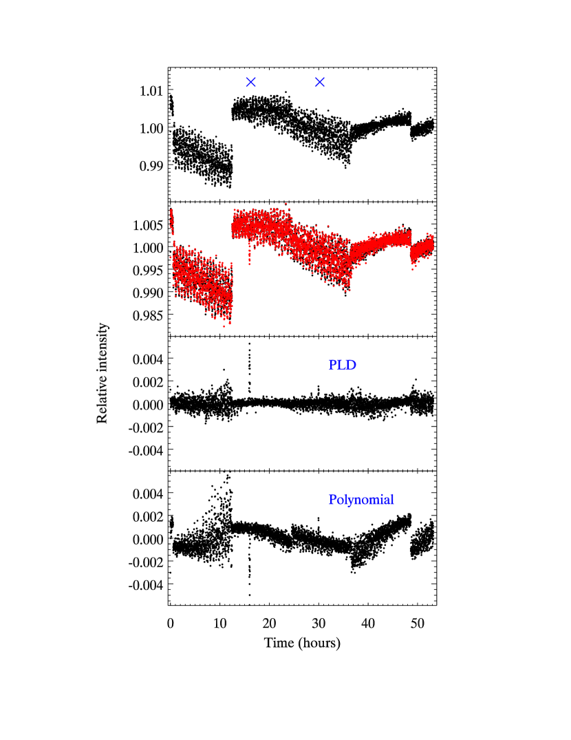
Some results from this test are illustrated in Figure 2. The top panel shows the photometry for the noiseless data prior to decorrelation. The second panel overlays (in red) the fitted function from the PLD regression onto the photometry. The two lowest panels show the residuals from the best fit for both the PLD and polynomial cases. Since there is no noise and no planet, all of the structure in the photometry is due to intra-pixel detector sensitivity variations. Neither technique removes all of the structure in the photometry, as evidenced by non-zero residuals in the two lowest panels of Figure 2. Certainly the detector sensitivity structure is not precisely quadratic, so the polynomial decorrelation is substantially imperfect. As for PLD, Eqs. (2) & (4) are accurate only in the limit of small changes in spatial position, and these test data exhibit relatively large fluctuations in position (up to 0.72 pixels in Y and 0.36 pixels in X). Nevertheless, the standard deviation of the PLD residuals (473 parts-per-million, ppm) is sufficiently small that it would not significantly limit most exoplanet observations, if combined in quadrature with photon noise. For reference, the photon noise of WASP-8, HAT-P-20, and WASP-14, in a 2-second frame time is 2150, 2500, and 2612 ppm, respectively. The standard deviation of the residuals from the polynomial fit in Figure 2 is 946 ppm, twice the PLD value. Using different centroiding and apertures, the polynomial decorrelation performs even more poorly compared to the PLD result, that is insensitive to the methodology of the photometry. Neither technique deals well with the noise-pixel spike due to PSF variation, but such spikes are rare in real data.

We used a quadratic polynomial for Figure 2 because that order is commonly used in real Spitzer decorrelations (e.g., Deming et al., 2011; Todorov et al., 2012, 2013). However, that’s arguably an unfair comparison because the quadratic decorrelation has only four position-dependent parameters, vs. nine for PLD. Therefore we also performed solutions using only the five brightest pixels in PLD, and comparing to polynomial decorrelations that are third and fourth order in both $X$ and $Y$. For the third and fourth order polynomials (6 and 8 parameters respectively), the residual error level is 601 and 553 ppm, respectively, whereas the 5-pixel PLD residual error is 511 ppm. Hence PLD is a more efficient decorrelation method than polynomials. Nevertheless, we note that polynomial decorrelations continue to be useful, for example in the recent re-analysis of GJ 436b (Lanotte et al., 2014). Moreover, in Sec. 7.2 of this paper we describe a sanity check of our HAT-P-20 results using a polynomial decorrelation.

The Figure 2 data exhibit much larger image motion than occurs in many, but not all, Spitzer eclipse observations. We examined how the amplitude of residuals in Figure 2 depends on the magnitude of the image motion. For image motion less than 0.03 pixels, the standard deviation of the residuals is 163 ppm, increasing smoothly to 461 ppm at 0.2 pixels of image motion. Beyond 0.2 pixels of image motion, the residual envelope varies less smoothly, but reaches 579 ppm at 0.3 pixels (not illustrated). Less than $\sim 0.2$ pixels of image motion is the region where our current version of PLD achieves optimum performance, but it still exceeds the performance of polynomial decorrelations even for image motion as large as 0.7 pixels.

We conclude that PLD produces a good fit to the intra-pixel detector structure, at least twice as good as a quadratic polynomial decorrelation, which is still commonly used in Spitzer analyses. However, in actual practice that factor of two will be significantly diluted by photon noise. On the other hand, PLD is minimally sensitive to the choice of centroiding and construction of the numerical aperture used in the photometry. (In Sec. 5.4 we show a PLD result that does not even require measuring the position of the star.)

4.3 Testing PLD with Synthetic Data for WASP-52b at 4.5 Microns

We also analyzed synthetic data containing both the planet (WASP-52b) as well as detector read noise and stellar photon noise. These data at 4.5 microns were analyzed by the community in the IRAC Workshop mentioned above, except that the noise model is now revised to properly account for the photon noise of previous Fowler samples. They comprise the same number of 2-second exposures as the noiseless data described above, covering a transit of the planet and two secondary eclipses. The planet in these data also exhibits a sinusoidal phase curve effect. We know in advance that the phase curve has a minimum at the center of transit and a maximum at the center of secondary eclipse. We also know that the synthetic transit occurs at phase 0.0 and uses no limb darkening. The eclipse is specified to occur exactly at phase 0.5, but the three amplitudes (transit and eclipse depth, and phase curve amplitude) are unknown.

We performed photometry on these data using a similar procedure as for the noiseless data, using both constant-radius and variable-radius apertures. In this case, we decorrelate the photometry using only PLD, and we compare the retrieved amplitudes to their input values in order to confirm that PLD is a valid method for decorrelating Spitzer data. Our fitting procedure is explained in Sec. 3.3. Table 1 lists the fitting parameters for these synthetic data, and the retrieved amplitudes in comparison to the known values.

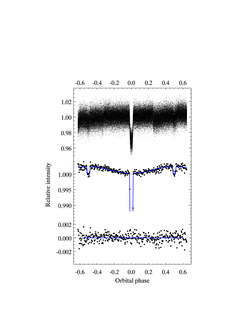
Figure 3 shows the photometry for WASP-52b prior to decorrelation (top panel), as well as the decorrelated binned data with best-fit orbital phase/transit/eclipse curve, and the residuals from the best binned fit. The retrieved amplitudes for the eclipse and transit parameters (Table 1) are in excellent agreement with the input values. Our retrieved eclipse depth differs from the input value by $0.2\sigma$, and the retrieved transit depth differs by $1.4\sigma$, both consistent with random noise. However, our retrieved phase curve amplitude differs from the input value by $3\sigma$. Our posterior distributions are very close to Gaussians, so that difference is very unlikely to be due to random error. The total range of image motion in these synthetic data exceeds 0.7 pixels, whereas Eq.(2) is only precise in the limit of small image motion. The real data we analyze all have less than a third as much image motion (see Table 2), and (as we show below) PLD produces robust results for the real eclipses. We conclude that PLD is a valid method for analyzing Spitzer exoplanet eclipse and transit data, but that it may require modification (e.g. adding higher order terms to Eqs. 2 & 4) in order to analyze phase curve data.

5 Testing PLD with Real Data

We have tested PLD with five sets of real data: GJ 436 (Ballard et al., 2010), CoRoT-2b (Deming et al., 2011), WASP-14b (Blecic et al., 2013), WASP-8b (Cubillos et al., 2013), and WASP-12b (Cowan et al., 2012; Stevenson et al., 2014). These data were chosen to represent a wide range of analysis situations. Although the purpose of these tests is primarily to validate PLD, we also obtain new astrophysical information, specifically a revised 3.6 $\mu$m eclipse depth for HAT-P-8b (Sec. 5.4), and recovery of a previous intractable eclipse of WASP-12b (Sec. 5.5).

The GJ 436 data were originally used to search for an additional planet (Ballard et al., 2010), and they contain no transits or eclipses. CoRoT-2b was observed at the start of Spitzer’s extended warm mission and analyzed using the polynomial method (Deming et al., 2011). WASP-14b (Blecic et al., 2013) and WASP-8b (Cubillos et al., 2013) were both analyzed quite recently, and used the BLISS method (Stevenson et al., 2012). WASP-8b at 3.6 $\mu$m was a challenging data set, which exhibited significant red noise in the normalized light curve (Cubillos et al., 2013). Cowan et al. (2012) found that the WASP-12b eclipse we analyze was especially difficult to fit, and they omitted that eclipse from their results, as did Stevenson et al. (2014). We thus challenge PLD with both variety and difficulty. Observational parameters for these five data sets are summarized in Table 2.

5.1 Testing PLD With Real Data: PLD vs. a Weighting Function

Our initial use of PLD showed immediately that it was a powerful technique. We therefore worried that it might be able to re-shape the data and produce an eclipse at any arbitrary orbital phase, even if no real eclipse was present. We alleviated this concern by applying PLD to the contiguous 33-hour time series data for GJ 436, used by Ballard et al. (2010) to introduce the weighting function method, and search for transits of a possible GJ 436c planet. These data contain no eclipses or transits, as Ballard et al. (2010) discuss.

The GJ 436 data comprise 488960 images (7640 data cubes each containing 64 frames). Since there are so many images with short exposure times (0.1 seconds), binning the data for the decorrelation is especially appropriate. Our fit procedure (Sec. 3.3) selects bins of 392 exposures (about 51 seconds of real time) for the decorrelation. Our solution quickly revealed a sharp transient rise in intensity over the first $\sim 30$ to $60$ minutes of the time series. Since this sharp increase is not adequately reproduced by the quadratic time dependence in our Eq.(4), we used an exponential time ramp, and we omitted the first 36 minutes of data that showed the greatest ramp effect.

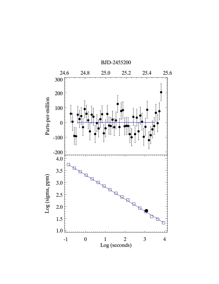
In this case, there is no eclipse or transit, and the best-fit eclipse depths are consistent with zero. The central phase can therefore take any value and still produce an equivalent fit. We use the regression solution to initialize three independent MCMC chains. The MCMC chains use the 392-point binning, and we find that the solution using that binning works well when applied to the unbinned data. We apply the best-fit binned solution to the original unbinned data to form residuals. We then re-bin those residuals on various time scales, as described in Sec. 3.3, to compare to Ballard et al. (2010), and to search for red noise that may remain in the results. We find a scatter of 65 ppm for 20-minute re-bins, shown in the top panel of Figure 4. That compares well to Ballard et al. (2010), who found 72 ppm on that time scale.

Applying our best-fit $c_{i}$ values and ramp parameters to the unbinned GJ 436 data, we re-binned the residuals on various time scales up to $2^{16}$ exposures (about 2.5 hours), and we find that the slope of $\log(\sigma)$ varies as $\log(N)$ with a slope of $-0.504$, essentially identical to the $-0.5$ slope expected for Poisson noise. The dependence of $\log(\sigma)$ on $\log(N)$ is shown in the lower panel of Figure 4. The unbinned residuals have a standard deviation of $0.00548$, 3% greater than the $0.0053$ obtained by Ballard et al. (2010). Because PLD operates on binned data, we do not fully correct the effect of short term pointing fluctuations. But the effective removal of red noise is a very acceptable trade for a 3% increase in the short-term scatter.

We conclude that PLD passes this test in the sense that it does not produce distortions in the data that would be mistaken for real transits or eclipses. We further conclude that the binned PLD solution effectively removes noise on longer time scales, albeit at the price of a small increase in noise on shorter time scales.

5.2 Testing PLD with Real Data: PLD vs. Polynomial Decorrelation for CoRoT-2b

Eclipses of CoRoT-2b were among the first data analyzed from the Warm phase of the Spitzer mission (Deming et al., 2011), and Hansen et al. (2014) mention CoRoT-2 as one of the most significant examples of deviation from a blackbody. We have tested PLD on the 3.6 $\mu$m eclipse of CoRoT-2b reported by Deming et al. (2011). The original analysis used the traditional polynomial method of decorrelating, with a quadratic function in Y, and a linear function in X. Our PLD result (not illustrated here) differs from the polynomial solution by less than $1\sigma$ in both the depth and phase of the eclipse. Like all of our eclipse fits in this paper, the characteristics and results of the fit are summarized in Table 1. The PLD solution yields a slope of $\log{\sigma}$ vs. $\log(N)$ of $-0.495$, statistically indistingusihable from $-0.5$. The slope derived from the original solution was not reported by Deming et al. (2011), but the errors on the eclipse depth and phase for the original fit are essentially the same as our current PLD solution. We conclude that our PLD analysis matches the original fit for this eclipse of CoRoT-2b, and again our PLD fit has essentially no red noise.

5.3 Testing PLD with Real Data: PLD vs. BLISS Mapping for WASP-14b

Turning to eclipse data that is more recent than CoRoT-2, we re-analyze the 3.6 $\mu$m eclipse of WASP-14b, as originally reported by Blecic et al. (2013). We choose WASP-14b because it has a slightly eccentric orbit, and the phase of the eclipse adds a useful dimension to the test. Moreover, the analysis described by Blecic et al. (2013) uses the well-documented and effective BLISS method (Stevenson et al., 2012) to correct for intra-pixel effects.

Our PLD decorrelation of WASP-14b used a 10-frame binning (about one-sixth of a data cube, 20 seconds of time), chosen by our PLD code to give the best red noise removal. Blecic et al. (2013) found that the choice of temporal ramp model was ambiguous, even using the Bayesian Information Criterion. We use a linear ramp and achieve a point-to-point scatter (standard deviation of the normalized residuals, $SDNR=3054$ ppm, Table 1). Our solution improves on the SDNR quoted by Blecic et al. (2013), who found values near $3310$ ppm (their Table 3). Like Blecic et al. (2013), we omit the first 1100 of 13760 frames from the solution. Following the regression solution of Eq.(4), we run three MCMC chains, each having $10^{6}$ steps, and we check convergence by comparing these independent chains. Our best-fit eclipse depth from the regression using the linear ramp is $1981\pm 66$ ppm, where the error comes from fitting a Gaussian to the posterior distribution. We obtain essentially the same eclipse depth from the centroid of the symmetric posterior distribution ($1968$ ppm). All of our PLD posterior distributions for the depth and central phase of all the eclipses we analyze are indistinguishable from Gaussians. Our result ($1981\pm 66$) ppm is in excellent agreement with Blecic et al. (2013), who quote an eclipse depth of $1900\pm 100$ ppm. Using the eccentric orbit model from Table 10 of Blecic et al. (2013), our best-fit central phase is $0.4833\pm 0.0004$, compared to $0.4825\pm 0.0003$ from Blecic et al. (2013), a $2\sigma$ difference. Both solutions confirm an eccentric orbit, and the central phases differ by a marginally significant amount.

Figure 5 shows our best-fit PLD eclipse for WASP-14b (top panel), re-binned to approximately the same time resolution used for Figure 8 of Blecic et al. (2013). Comparing to the overplotted (gray) points from Blecic et al. (2013), the PLD fit has fewer outliers, but is otherwise very similar. The middle panel shows the residuals from our fit, and the lower panel shows the standard deviation of our residuals when binned on time scales from one frame (2 seconds) to $2^{11}$ frames (about 4100 seconds, including overhead). The best-fit slope to the binned standard deviations on the lower panel of Figure 5 ($-0.494$) is statistically indistinguishable from Poisson noise ($-0.5$).

We conclude that our PLD analysis gives an eclipse depth consistent with previous work, and again we find that it attenuates red noise.

5.4 Testing PLD with Real Data: PLD vs. BLISS Mapping for WASP-8b

Another challenging test of PLD is the 3.6 $\mu$m eclipse of WASP-8b reported by Cubillos et al. (2013). Those authors utilized a BLISS technique to analyze this eclipse, but found significant red noise remaining after the decorrelation. Moreover, they found an eclipse depth that they described as ‘anomalously high’, requiring some tension in the astrophysics to account for it (Sec. 6 of their paper). We have applied PLD to this eclipse, using a quadratic temporal ramp as per the original analysis (Cubillos et al., 2013). Both the original, and our re-analysis, omit some frames at the start of the time series, which is a normal procedure for Spitzer analyses because there are transient effects at the outset.

This star has a possibly bound M-dwarf companion 5 arcsec distant, and 2.1 magnitudes fainter in K-band (Queloz et al., 2010; Cubillos et al., 2013). The companion lies outside of our photometry apertures, but can contribute scattered and diffracted light. Appealing to symmetry, we measure the scattered and diffracted light from WASP-8 itself, by placing a numerical aperture at the distance of the companion, but on the opposite side from it. We calculate a correction factor using that fractional light contribution together with the relative brightness of WASP-8 and the companion. We apply the dilution correction to the eclipse depth after the decorrelation and fitting process, not to the photometry. The correction we calculate is 2.5%.

Our PLD fit is listed in Table 1, and shown in Figure 6. We find a significantly cleaner fit to the eclipse with fewer outliers compared to the original fit from Cubillos et al. (2013) (compare black and gray points in the top panel of Figure 6.) For WASP-8, as well as HAT-20 (discussed below), eclipses shown graphically in our Figures do not include correction for the companion stars, but that correction is included in the Table 1 eclipse depths. Our code chooses 148 point binning (1.05 minutes) for our WASP-8 solution, i.e. slightly more than two Spitzer data cubes. Applying that binned solution to our unbinned photometry, we find a SDNR$=5414$ ppm, vs. $5377$ from Cubillos et al. (2013), a 0.7% difference. Our PLD solution yields a slope of the binned-$\sigma$ relation of $-0.492$, showing essentially no red noise. Our eclipse depth is $906\pm 74$ ppm, vs. $1130\pm 180$ from Cubillos et al. (2013), a difference that is 1.2 times their error. Cubillos et al. (2013) determine the precision of their eclipse depth by accounting for correlations in their residuals using the $\beta$ parameter method of Winn et al. (2008). Our error is based solely on our MCMC posterior distribution for eclipse depth, since we find no significant correlation in the residuals. Our eclipse depth is consistent with the atmospheric models for the planet shown in Figure 8 of Cubillos et al. (2013), and reduces the tension with the astrophysics of the exoplanetary atmosphere that they discuss. Although we believe that the eclipse depth from Cubillos et al. (2013) is too large, we point out that their excellent error analysis encompasses our revised eclipse depth.

Sec. 2 mentions that it might be possible to obtain good photometry from the sum of the $3\times 3$-pixels in Eq.(3). As the stellar image moves, the fraction of total light encapsulated by a $3\times 3$-pixel sum will vary, because the image is moving but the pixels are stationary. It is reasonable to hypothesize that Eq.(4) will correct for variable light loss, just as it corrects for the intra-pixel sensitivity effect. If so, it may be possible to obtain excellent eclipse results by simply summing the pixels that contain the star, without implementing conventional aperture photometry. Simple sum-of-pixels photometry has distinct advantages. It obviates all of the issues associated with the best way to measure the stellar centroid, and other effects such as the ‘pixelization’ discussed by Stevenson et al. (2012) become irrelevant.

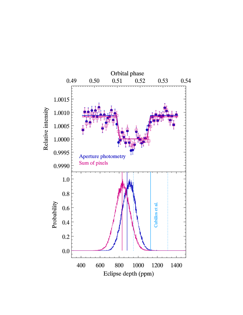
Sum-of-pixels photometry is most appropriate for bright stars, where the stellar intensity greatly exceeds the sky background. For relatively faint stars where background fluctuations contribute significantly to the noise, aperture photometry remains desirable in order to optimize the star-to-background ratio. For that reason, we continue to rely on aperture photometry as a primary tool in our PLD analyses, but we here test sum-of-pixels photometry for our brightest eclipsing system, WASP-8. Figure 7 compares the aperture photometry for WASP-8 (Figure 6) with an independent decorrelation based on replacing the aperture photometry with the denominator of Eq.(3), i.e. using the sum of a $3\times 3$-pixel box. The results are very similar (Table 1); the eclipse depths differ by only 54 ppm, less than $1\sigma$, and the Gaussian-shaped posterior distributions for eclipse depth (Figure 7) overlap significantly. The slopes of the binned-sigma relations (Table 1) are both indistinguishable from $-0.5$. Moreover, both results for the eclipse depth are in good agreement with the modeled spectrum shown by Cubillos et al. (2013), eliminating the need to invoke unusual astrophysics.

We conclude that PLD permits robust photometry of bright stars, without the need to measure the position of the image.

5.5 Testing PLD with Real Data: WASP-12b

Cowan et al. (2012) studied the phase variation of thermal emission from the very hot planet WASP-12b, and their Spitzer data contained two eclipses of the planet at 3.6 $\mu$m. The first of these eclipses exhibited ‘highly correlated residuals’ after their polynomial and weighting function decorrelations (Cowan et al., 2012). Their depth for this problematic eclipse was significantly less ($0.0030$ versus $0.0038$) than a previously analysed eclipse of this planet also at 3.6 $\mu$m (Campo et al., 2011). Stevenson et al. (2014) declined to include this eclipse in their recent re-analysis of WASP-12b data. It therefore makes a challenging case for our PLD analysis.

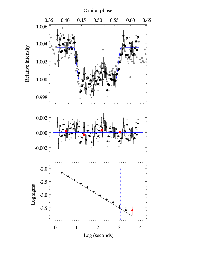
Our best-fit solution (Figure 8) for this eclipse yields a depth of $0.00363\pm 0.00018$, consistent (at $1\sigma$) with the second eclipse in the data analyzed by Cowan et al. (2012) ($0.0038\pm 0.0004$). We also agree with other 3.6 $\mu$m eclipses analyzed by Campo et al. (2011) ($0.00379\pm 0.00013$), and approximately with Stevenson et al. (2014) ($0.0041\pm 0.0002$, $0.0038\pm 0.0002$, and $0.0036\pm 0.0002$). Our best-fit eclipse phase using the ephemeris from Chan et al. (2011) is consistent with a circular orbit (Campo et al., 2011). Although the eclipse depths quoted above do not include correction for the dilution by the companion star, that correction is included in Table 1. Since our average photometric aperture is close to the 3.0 pixels used by Stevenson et al. (2014), we adopt their dilution correction factor ($1.1149$). Our corrected eclipse depth ($4051\pm 202$ ppm) agrees well with the corrected average eclipse depth (3 eclipses) from Stevenson et al. (2014) ($4210\pm 110$ ppm), and one eclipse from Campo et al. (2011) ($3790\pm 130$ ppm).

Our result for this eclipse is compared to Cowan et al. (2012) in Figure 8. Some important differences in method are that Cowan et al. (2012) were fitting an entire orbit of data, and they used a planetary phase function, but no instrumental temporal ramp. We fit to only the data between phases 0.4 and 0.6, and we use a linear temporal ramp in Eq.(4). Those differences alone will tend to give us better results for the eclipse, but our intent is primarily to demonstrate a successful PLD analysis of this eclipse, and only secondarily to compare to Cowan et al. (2012). The fit from Cowan et al. (2012) exhibits a slope in the residuals during the eclipse, when the planet is not contributing. Figure 8 shows that we find significantly less slope, as can be seen particularly just prior to egress. We also find less scatter, and very little correlation in the residuals. Our slope for the binned residuals (bottom panel of Figure 8) is $-0.470$. We conclude that PLD can successfully fit this difficult eclipse data set.

6 Observations of HAT-P-20b, and Initial Data Processing

We now turn to HAT-P-20b (Bakos et al., 2011), and apply PLD to this moderately-irradiated giant exoplanet. We here analyze four eclipses that have not previously been published.

We observed two eclipses of HAT-P-20b in each Warm Spitzer band, in program 80219 (H. Knutson, P.I.), using subarray mode. Times of the observations are given in Table 3. Our analysis used the BCD data cubes, each having 64 frames of 2-second exposures. We find and correct discrepant pixels due to energetic particle hits or other transient effects using a median filter applied to each pixel as a function of time. We construct a 5-pixel running median of each pixel’s intensity within a given $32\times 32\times 64$-pixel data cube, and we set $4\sigma$-discrepant pixels to the median value. We similarly apply a $4\sigma$ median filter to the photometry and image positions internal to each data cube.

For both HAT-P-20b and the tests using synthetic and archival data, we subtract a background level from each frame of the 64-frame data cube, by fitting a histogram to pixels in the four $6\times 6\times 64$-pixel spatial corners of each data cube. We use this procedure to minimize background contribution from HAT-P-20 itself and from a companion star (Bakos et al., 2011). After the background subtraction, we locate the center of the HAT-P-20 stellar image using both a 2-D Gaussian fit, and also a center-of-light calculation. We measure the flux using both constant-radius and variable-radius apertures, as described in Sec. 4.2.

HAT-P-20’s companion star is physically bound (Ngo et al., 2014), about one magnitude fainter, and 6.9 arc-sec (5.7 pixels) distant. As for the WASP-8 case, we estimated the (small) contribution of diffracted light from the companion by measuring the flux from HAT-P-20 6.9 arc-sec in the opposite direction from the companion, using the same photometric apertures that we adopted for HAT-P-20. After adjusting for the brightness of the companion relative to HAT-P-20, we find that the depth of the HAT-P-20 eclipses are diluted by 0.63% and 1.56% at 3.6- and 4.5 $\mu$m respectively, and we applied this correction to our results after the decorrelating and fitting process. We also used photometry of the companion star as a check on our results for the HAT-P-20 eclipses, as described in Sec. 7.2.

7 Eclipses of HAT-P-20b

Table 1 lists the parameters of the best-fit for each eclipse of HAT-P-20. As for previous eclipses, all of our PLD solutions for HAT-20 have a slope of $\log{\sigma}$ vs. $\log{N}$ close to the Poisson value of $-0.5$, but we do not illustrate the $\sigma(N)$ relations in these cases.

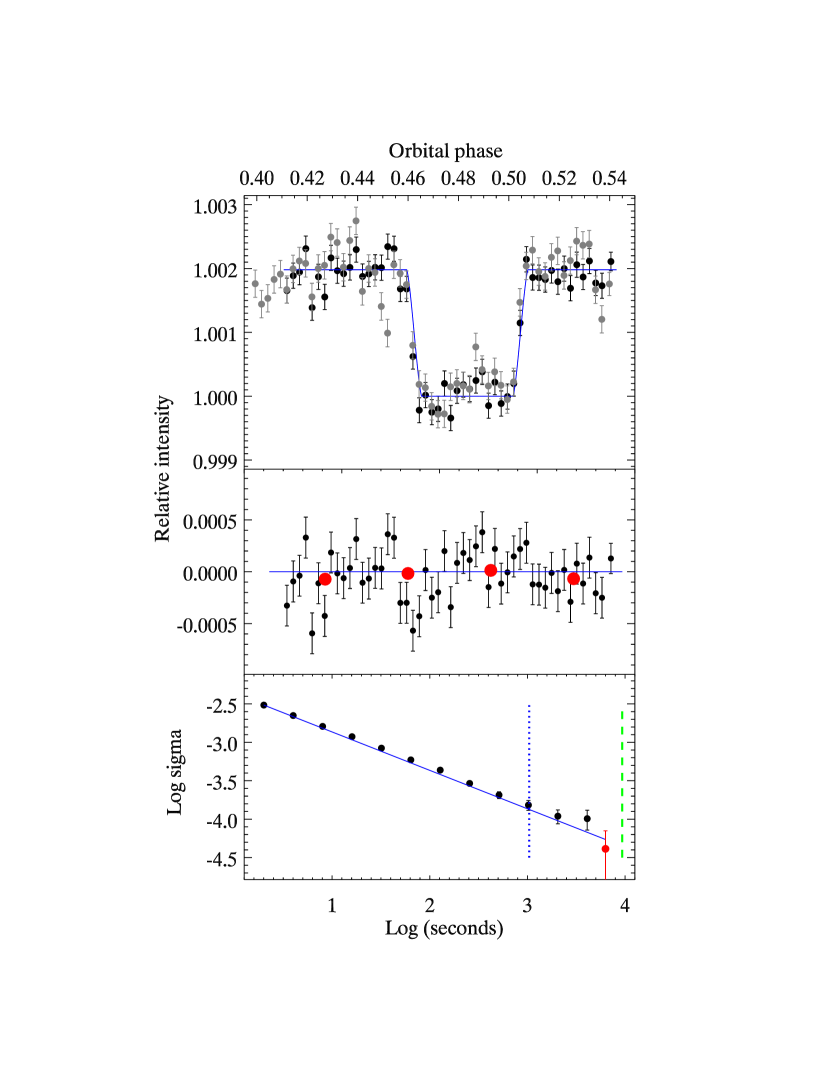
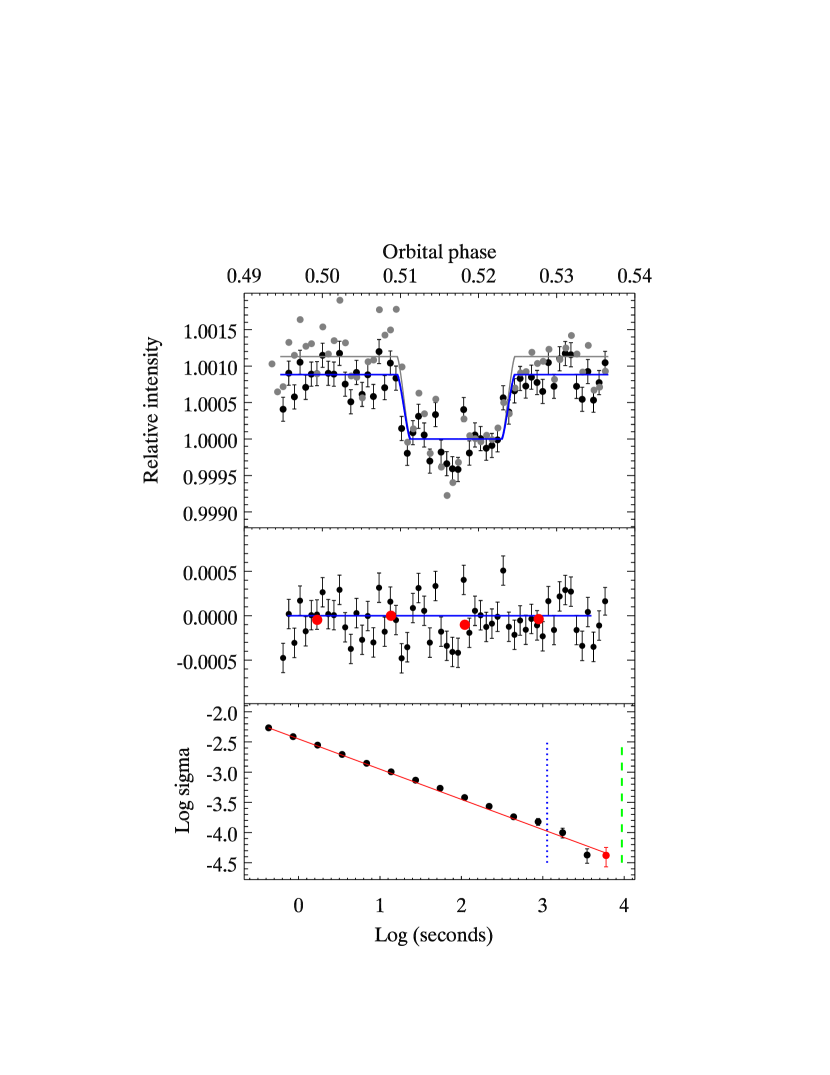
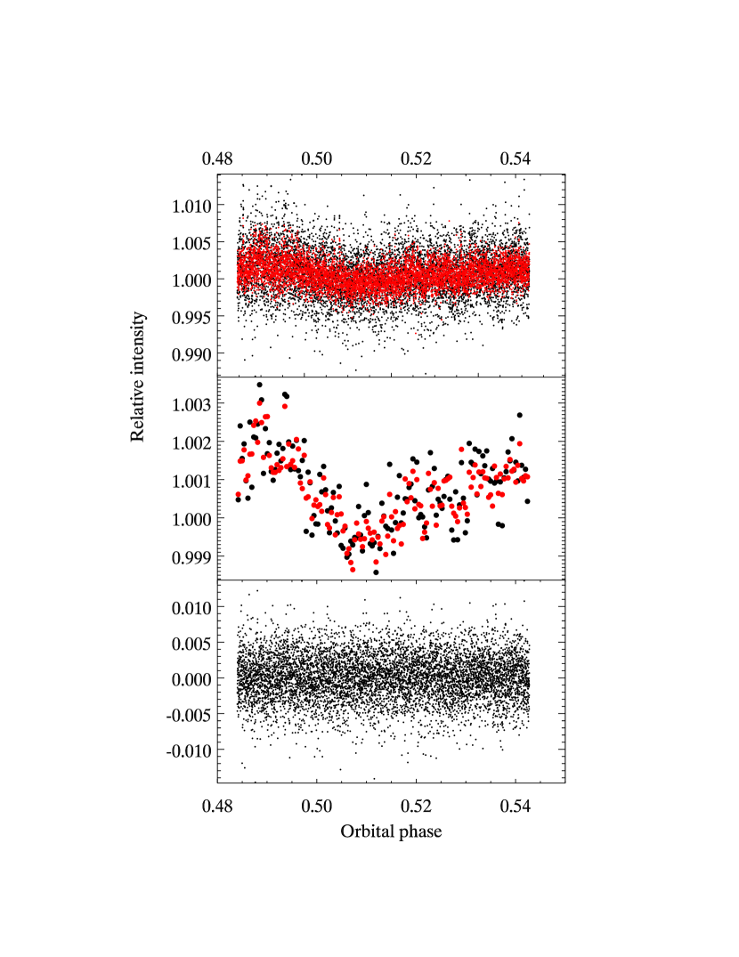
Figure 9 illustrates the unbinned vs. binned aspect of our fits, using the second HAT-20 eclipse at 3.6 $\mu$m, that has the most binning (maximum binning facilitates seeing the difference). The top panel shows the unbinned photometry overlaid point-by-point with the best fit calculated using the $c_{i}$ coefficients from the binned fit. The middle panel shows the binned data and the binned fit, using a 48-exposure binning selected by our fit procedure (Sec. 3.3). The lower panel shows the residuals for the unbinned case (data minus fit), showing the close resemblence of the residuals to white noise.

7.1 3.6 $\mu$m Eclipses

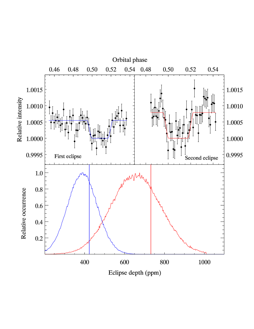
Figure 10 shows the two eclipses at 3.6 $\mu$m. Our analysis code selects a wide variety of bin sizes when doing the HAT-P-20 fits (1, 2, 32, and 48 exposures). Consquently, for Figure 10 we re-bin the photometry so that 50 points span the data. The lower panel of Figure 10 shows the posterior distributions from the MCMC chains. One chain per eclipse is illustrated, but we used three independent chains of $10^{6}$ steps for each eclipse and their distributions were closely identical. The two eclipses at this wavelength differ in their retrieved depth, but the difference is only 246 ppm (see Table 1). Since these are independent events, the error on the difference in eclipse depths equals the quadrature sum of the errors on the individual eclipses, which is 163 ppm. So the difference in the two eclipse depths at 3.6 $\mu$m is $1.5\sigma$, consistent with random noise.

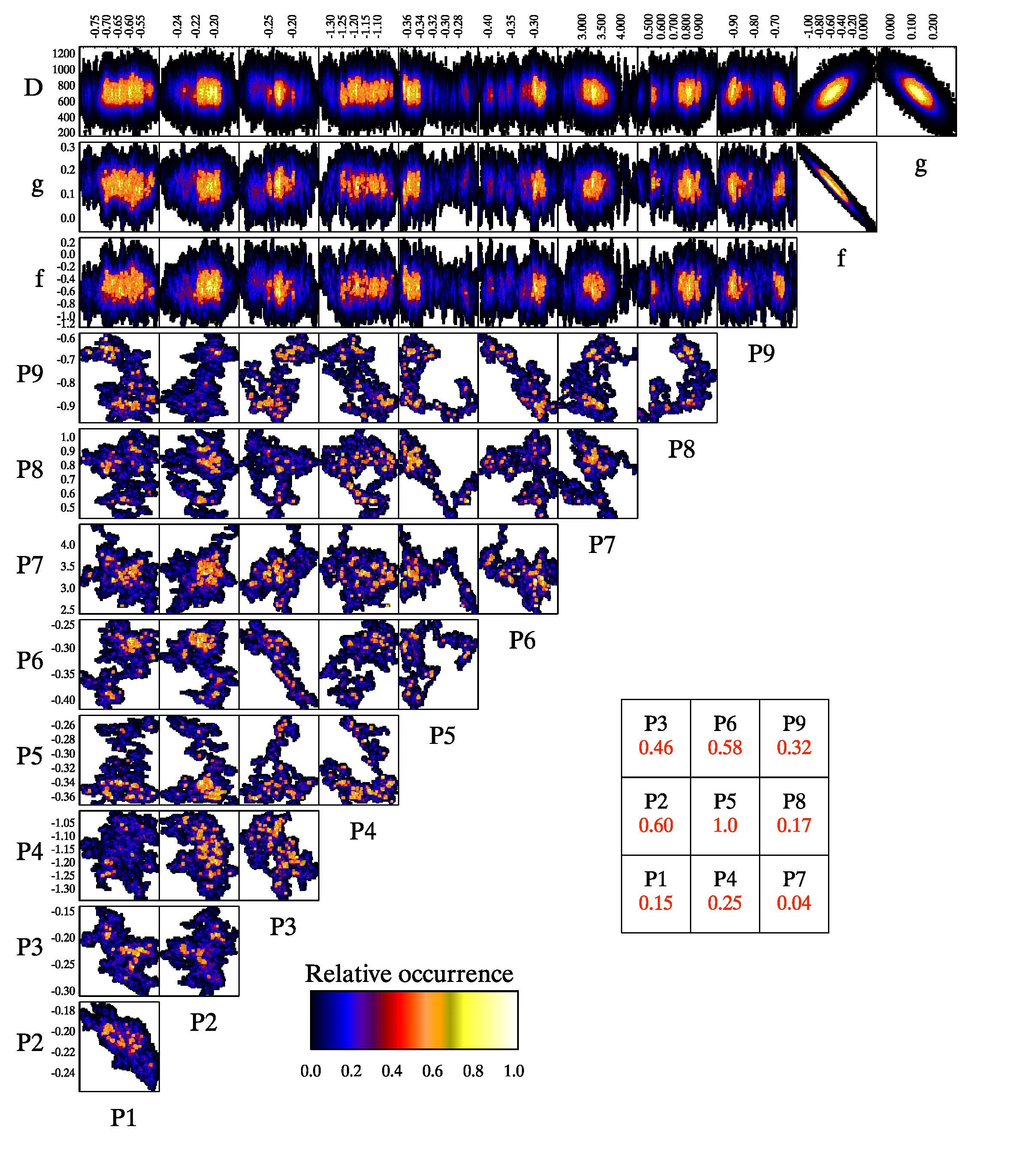
We found one anomaly in our PLD solutions. The eclipse depth for the second eclipse at 3.6 $\mu$m is degenerate with the purely temporal (baseline) terms in Eq.(4). We use a quadratic temporal ramp in the solution, but the degeneracy remains if we use only a linear ramp (and the fit is worse). We also explored using an exponential ramp in Eq.(4) for this eclipse, but we find that it does not produce an acceptable fit. Examining the fit closely, we found that the data required a ‘U’-shaped baseline, and an exponential cannot produce that shape. The ’U’-shape is evident on the middle panel of Figure 9. We therefore adopt a quadratic temporal ramp, and we tolerate the degeneracy because it is included in the error derived from the posterior distributions - note the broader distribution for the second 3.6 $\mu$m eclipse on Figure 10. Figure 11 shows the MCMC chain values for the baseline coefficients and the pixel ($c_{i}$) coefficients for this eclipse. The degeneracy is obvious from the correlations shown in panels on the top right, giving the linear and quadratic coefficients of time. Note also that the linear coefficient is correlated with the quadratic coefficient, since the fit can compensate for less or more baseline curvature by varying the baseline slope. None of the $c_{i}$ coefficients exhibit any correlation with the eclipse depth. Nor do we find correlations between the $c_{i}$ and the eclipse depths for any data set we have analyzed.

7.2 4.5 $\mu$m Eclipses

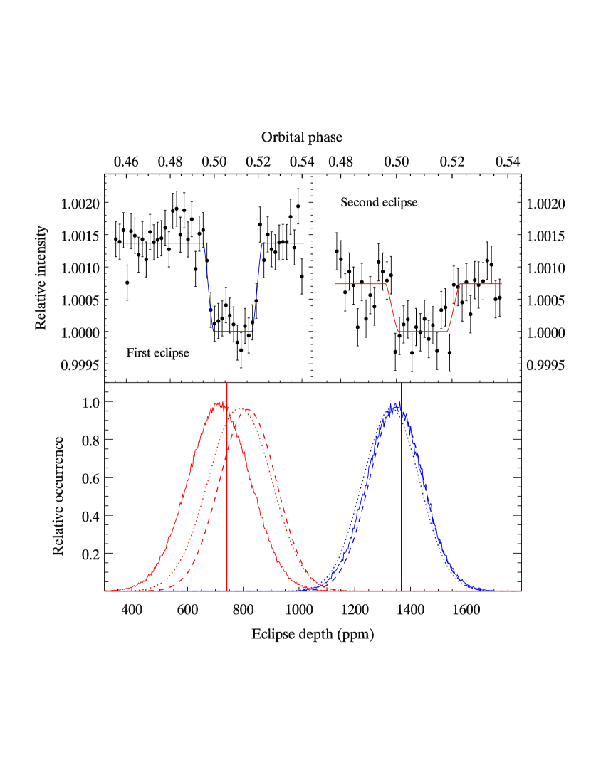
Figure 12 shows the two eclipses at 4.5 $\mu$m. For visual clarity, they are binned to 50 (first eclipse) and 40 points (second eclipse having less data). In this case, the difference in eclipse depths (625 ppm) is about four times the error of the difference (154 ppm). This $4\sigma$ difference is not a statistical fluctuation, given that the posterior distributions are closely Gaussian. Either the errors are underestimated, or the planet is variable. We considered possible variable dilution by scattered light from the companion star. Because the companion is 6.8 arc-sec distant from HAT-P-20, its scattered light contribution is only about 1.5% of HAT-P-20, and our measurements show that it does not vary sufficiently to significantly affect the relative eclipse depths at either 3.6 or 4.5 $\mu$m. Moreover, we find no degeneracies or any other anomalies in our PLD fits at this wavelength, in contrast with 3.6 $\mu$m - where the eclipse depths are in good agreement in spite of the degeneracy discussed above.

If the errors are underestimated, the most likely reason is that the results depend on features of the data or decorrelation process that are not included in the variations probed by the Markov chains. One such possibility is the choice of pixels used in the PLD decorrelation. All of our fits listed in Table 1 use 9 pixels, usually in a $3\times 3$-box centered on the star. Since the corner pixels contain the least flux, it is arguably possible that they are unnecessary to the fit, and might even be perturbing it in an undesirable way.

To explore the robustness of the PLD fits, we re-fit both eclipses with the corner pixels omitted from the PLD solution. The posterior distributions for the no-corner fits are plotted with dashed lines on the lower panel of Figure 12. They are shifted slightly with respect to the $3\times 3$-pixel solutions, but still indicate different depths for the two eclipses. Also, the central phases for all of the HAT-P-20b eclipses (Table 1) are very consistent. We conducted additional checks such as forcing our code to use the same parameters (binning, centroiding, aperture type and size) for both eclipses, and the difference between the two eclipses persists. We also implemented a conventional polynomial decorrelation, by replacing the $\hat{P}_{i}^{t}$ values in Eq.(4) with image centroid coordinates ($X$, $X^{2}$, $Y$, and $Y^{2}$). Those posterior distribution are shown as dotted lines on Figure 12, and are in good agreement with the PLD results.

In principle, if our values for the average brightness of HAT-P-20’s host star at each eclipse were in error by a large amount, the resultant incorrect normalization factors could lead to large errors in the eclipse depths. We checked this by comparing HAT-P-20 to the companion star. We find the average brightness of HAT-P-20 decreased by 1.6% from the first to the second eclipse at 4.5 $\mu$m, and the companion decreased by 1.9%. At 3.6 $\mu$m, HAT-P-20 decreased by 7.8%, versus a 1.6% increase for the companion. Although the relatively large variation of HAT-P-20’s absolute brightness at 3.6 $\mu$m is puzzling, it is not large enough to affect the eclipse, and the two 3.6 $\mu$m eclipse depths are consistent within the errors, as discussed in Sec. 7.1. Variation in the absolute brightness of HAT-P-20 at 4.5 $\mu$m is consistent with the variation seen in the brightness of the optical companion, so there is no reason to attribute our result to errors in normalizing the photoemtry.

We also decorrelated the photometry of the companion star using the same PLD code as for HAT-P-20. We solve for the depth of an ‘eclipse’ in the companion data, constraining it to have the same orbital phase as observed for HAT-P-20’s eclipse (Table 4), and using a simple linear ramp in time. These decorrelated results all show flat time series, with a per-exposure scatter that exceeds the photon noise by an average of 29% and 13% at 3.6- and 4.5 $\mu$m, respectively. The slopes of the binned-$\sigma$ relations were better than -0.48 in all four cases, and the derived ‘eclipse’ depths were consistent with zero. Those depths were (for the same order as Table 3): $+46\pm 99$ ppm, $-122\pm 78$ ppm, $+68\pm 118$ ppm, and $-181\pm 113$ ppm.

We conclude that the difference in HAT-P-20’s 4.5 $\mu$m eclipse depths is not due to the PLD analyses. In order to infer the average atmospheric properties of HAT-P-20b, we calculate the average eclipse depth in each band, weighting each eclipse by the inverse of its variance. Those average values are listed in Table 4.

8 Implications for the Atmosphere of HAT-P-20b

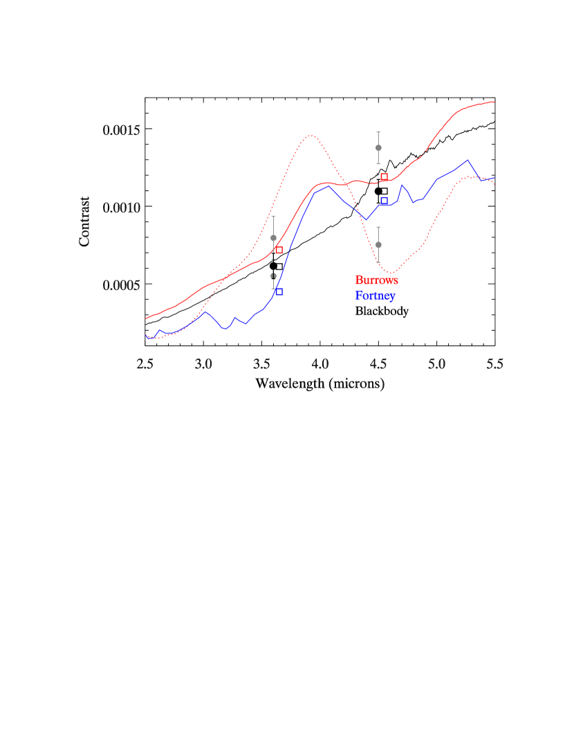
Figure 13 shows our results for eclipse depths of HAT-P-20b in comparison to the contrast from a best-fit blackbody temperature of $1134\pm 29$ K. We estimated the error for that best-fitting blackbody by increasing the observed error at 4.5 $\mu$m to allow for the discordant eclipse depths at that wavelength. The best-fit blackbody temperature is essentially identical to the $T=1157$ K that would prevail if HAT-P-20b absorbs stellar energy with zero albedo, and re-radiates uniformly over the star-facing hemisphere. Cowan & Agol (2012) studied the statistics of heat re-distribution using secondary eclipse data, and Perez-Becker & Showman (2013) studied heat re-distribution using phase curves. Both find a tendency for the most strongly-irradiated planets to circulate heat with the least efficiency. A strongly-irradiated planet will be hot, and the radiative time constant decreases strongly with temperature. A short radiative time constant in turn implies that the planet re-radiates incident stellar energy before hydrodynamics can advect it to the anti-stellar hemisphere (Showman & Guillot, 2002; Cowan & Agol, 2012; Perez-Becker & Showman, 2013). HAT-P-20b is irradiated at only a modest level (equilibrium temperature 970K for 2-hemisphere re-radiation), but the high density and probable high metallicity of the planet should produce higher atmospheric opacity. We suggest that high opacity may sufficiently compensate for less irradiation, keeping the radiative time scale short compared to advection. Lewis et al. (2010) studied the day-night flux difference for GJ 436b using a numerical hydrodynamic model, and found that that the difference does increase with metallicity, but only by $\sim 30\%$, less than needed to account for HAT-P-20b. However, HAT-P-20b is hotter than GJ 436b, and the effect of metallicity should be larger at higher temperature. Also, the atmosphere of HAT-P-20b may contain abundant absorbing clouds because the temperature is below the condensation point for many compounds, and the metallicity may be high. In that case, cloud absorpion could further increase the day-night temperature difference.

Figure 13 includes two solar metallicity model atmospheres (Burrows et al., 2006, 2007; Fortney et al., 2005, 2006a, 2006b, 2008) that have minimal heat re-distribution. These models have relatively strong absorption in the 4.5 $\mu$m band due to carbon monoxide and water vapor (Sharp & Burrows, 2007), and they therefore deviate from a blackbody model. However, we find that a blackbody at $1134$ K is essentially a perfect fit to our average eclipse depths, matching each value in Table 4 to better than $1\sigma$. This blackbody-like behavior frustrates our inital motivation to find strong molecular absorption in a modestly-irradiated, metal-rich, giant exoplanet. However, our work does suggest possible variability in the eclipse spectrum of this planet.

Assuming solar composition, the 4.5 $\mu$m Spitzer band is formed higher in the exoplanetary atmosphere than is the 3.6 $\mu$m band. If conditions in the atmosphere vary strongly with time, then we expect the greatest variability at the highest altitude, because low density regions are more easily perturbed than high density regions. Two mechanisms can translate atmospheric variability to the emergent spectrum: patchy clouds, and hot spots at any altitude (Morley et al., 2014). Hot spots at high altitude are qualitatively consistent with our result of divergent eclipse depths at 4.5 $\mu$m, but the requisite amplitude seems unrealistic. Brown dwarfs are often found to exhibit variability due to rotational modulation, but HAT-P-20b would have to exhibit a much greater amplitude of variability than do brown dwarfs. The large amplitude of apparent variability that we observe is difficult to reconcile with our expectations for hot Jupiter atmospheres.

An arguably more plausible explanation for eclipse depth variability is circum-planetary thermal or fluorescent emission in the fundamental band of CO, due to planetary mass loss or ongoing accretion. The CO band falls in Spitzer’s 4.5 $\mu$m bandpass, and was considered as producing an anomalous eclipse of CoRoT-2b by Deming et al. (2011). HAT-20b is likely to be a high-metallicity planet, and the CO abundance will increase approximately as the square of the metallicity, so large CO column densities are plausible. Moreover, if circum-planetary emission contaminates the 4.5 $\mu$m eclipse depth, then our inferred temperature for the planet will be biased too high, and the efficiency of longitudinal heat transfer could be higher, making that aspect of the observations less puzzling.

Claiming a high degree of variability in eclipse depth requires strong evidence, and two eclipses - no matter how thoroughly they are analyzed - are insufficient to conclude that this planet is variable. However, our results are sufficient to warrant further eclipse monitoring of HAT-P-20b. Our working hypothesis is that circum-planetary emission in the fundamental CO band may be important. Monitoring of the 4.5 $\mu$m eclipse depth by Spitzer can establish whether there is real photometric variability, but spectroscopic observations using JWST will be necessary to detect possible CO emission.

9 Implications for the Orbit of HAT-P-20b

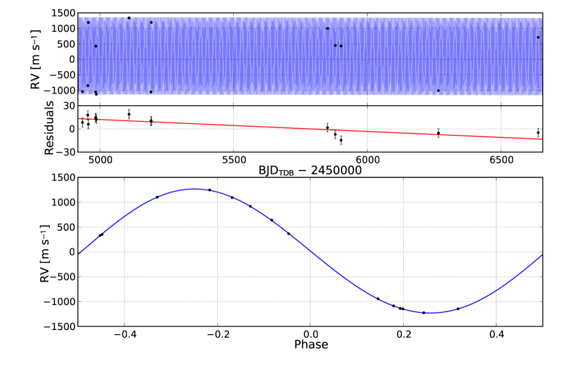
The central phase of all four eclipses we observe is consistently later than the $0.5$ value for a circular orbit (Tables 1 & 4). We first ask whether this could be due to the accumulated uncertainty in the orbital period. We use the most precise available orbital period from Granata et al. (2014), but even the discovery-era period error given by Bakos et al. (2011) ($4.0\times 10^{-6}$ days) is already an order of magnitude too small to account for the phase shifts we observe. Using the ephemeris from Granata et al. (2014), we calculate the average eclipse phase at each wavelength, and the grand average for all four eclipses. The results are listed in Table 4; we find a grand average orbital phase of $0.50843\pm 0.00041$, and the uncertainty in the ephemeris from Granata et al. (2014) contributes negligibly. The light travel time across the orbit is $36$ seconds, hence the eclipse for a circular orbit would occur at phase $0.50014$, and our measured phase corresponds to $e\cos(\omega)=0.0130\pm 0.0006$. Radial velocity observations of this system were analyzed by Knutson et al. (2014), who derived $e\cos(\omega)=0.013^{+0.0023}_{-0.0025}$, closely consistent with our secondary eclipse timings. To close the loop on this system, we have derived new orbital parameters using a joint MCMC fit of the RV and secondary eclipse timings, as described by Knutson et al. (2014). The results from this fit are given in Table 5, and illustrated in Figure 14. The priors used in the fit are the RV observations reported by Knutson et al. (2014), the transit ephemeris from Granata et al. (2014), and the secondary eclipse timings from Table 4. Our result of $e\cos{\omega}=0.01352^{+0.00054}_{-0.00057}$ establishes the small eccentricity of the orbit to high statistical confidence. Given the existence of a bound stellar companion, HAT-P-20b is another excellent candidate for orbital evolution via Kozai migration (Fabrycky & Tremaine, 2007), or other three-body mechanism.

10 Summary

In this paper we have introduced a new method for correcting the intra-pixel effect in Spitzer photometry at 3.6- and 4.5 $\mu$m, that we call pixel-level decorrelation (PLD). PLD differs fundamentally from all previous methods because it removes the effect of positional jitter without explicitly using the position of the stellar image. We argued the conceptual advantages of PLD (Sec. 2), and we have tested it using both synthetic (Sec. 4) and real data (Sec. 5). We point out that all methods to decorrelate Spitzer photometry at these wavelengths are subject to the mathematical reality that the solution is a function of the time scale (i.e., degree of data binning) because both the dependent and independent variables contain random error (Sec. 3.1). Moreover, there are physical reasons to apply PLD to binned data, discussed in Sec. 3.2. Our fitting procedure finds the best fit to Spitzer data by considering a range of time scales, yielding a broad bandwidth solution having minimal red noise (Sec. 3.3).

Our tests of PLD exploited a new capability to generate synthetic Spitzer data, developed at the Spitzer Science Center. These tests began with synthetic data having no planet and no photon noise, thereby isolating the intra-pixel detector effect (Sec. 4.2). We tested PLD using synthetic data for WASP-52b, and we recovered the correct transit and eclipse depth to within $1\sigma$ (Sec. 4.3). We also recovered the phase curve amplitude of WASP-52, but our PLD result was off by $3\sigma$. The large image motion that accumulates over the time scale of a phase curve measurement is beyond the range of applicability for our current version of PLD, so it is not yet applicable to phase curve measurements. However, PLD is very robust for transits and eclipses. We tested PLD on five real systems. In cases where there is no reason to doubt previous measurements, our PLD result agrees with published results. These cases include GJ 436b (Sec. 5.1), CoRoT-2b (Sec. 5.2), and WASP-14b (Sec. 5.3). In two systems (WASP-8b, Sec. 5.4, and WASP-12b, Sec. 5.5) our PLD eclipse depths are more astrophysically plausible than the original published results, and have smaller random errors. For example, our error for WASP-8b at 3.6 $\mu$m improves on the result from Cubillos et al. (2013) by more than a factor of two, and our eclipse depth agrees well with the same modeled spectrum they used to account for eclipses in other Spitzer bands.

We apply our PLD analysis to two eclipses of HAT-P-20b at each Spitzer wavelength (Secs. 6 and 7). We find that the average spectrum of the planet is very close to a blackbody at $1134\pm 29$K, indicating a low albedo and little if any longitudinal re-distribution of stellar heating (Sec. 8). Our results at 4.5 $\mu$m (Sec. 7.2) yield two eclipse depths that differ by $4\sigma$. Although two eclipses are not enough to conclude that the planet’s spectrum is variable, we do conclude that there is justification to monitor the eclipse depth at 4.5 $\mu$m using Spitzer, and to search for circumplanetary emission in the 1-0 fundamental CO band using JWST. All four of our measured eclipses occur at a phase later than 0.5, indicating a slightly elliptical orbit. A joint MCMC fit of our eclipse times with RV observations and and the transit time yields $e\cos{\omega}=0.01352^{+0.00054}_{-0.00057}$, and establishes the small eccentricity of the orbit to high statistical confidence (Sec. 9). Given the existence of a physically bound companion star, HAT-P-20b is another candidate for orbital evolution via Kozai migration, or other 3-body process.

11 Acknowledgements

We thank Jasmina Blecic, Patricio Cubillos, and Joseph Harrington for sending us digital version of their results, used in Figures 5-7, and we thank Julie Moses for comments on this paper. This work is based on observations made with the Spitzer Space Telescope, which is operated by the Jet Propulsion Laboratory, California Institute of Technology, under a contract with NASA.

Figure 1: Graphical illustration of how PLD works, for the 2nd eclipse of HAT-P-20b at 3.6 $\mu$m (see Table 3, and Figure 10). The time series for the relative values of the normalized pixels ($\hat{P}_{i}^{t}$, see Eq. 3), are each multiplied by the $c_{i}$ coefficients, and added to the eclipse model and the temporal ramp ($t=$ time, or orbital phase) to produce the total fit, shown in red overlying the aperture photometry at the top. (These are the actual $\hat{P}_{i}^{t}$ time series used in the solution, but for clarity we here exaggerate the curvature of the temporal ramp.) The inset at the lower left shows the pixel designations. In this case nine pixels are used, in a $3\times 3$ spatial arrangement. Nothing limits PLD to using nine pixels. The number and spatial arrangement of the pixels that are actually used is determined by the distribution of intensity in the stellar image.

Figure 2: Photometry of synthetic 3.6 $\mu$m data for WASP-52, with the photon noise turned off and the planet removed. All of the fluctuations in the top panel are due to the interaction of the telescope PSF with the spatial structure of the detector. The blue Xs mark the times where PSF fluctuations were inserted into the data. The second panel overlays the PLD fit from Eq.(4), and the two lowest panels show the residuals for the PLD fit and also for a fit using a second order polynomial in both X and Y. Note the different ordinate scales, especially for for lower panels.

Figure 3: Fitting to photometry of synthetic 4.5 $\mu$m data for WASP-52b, with photon and detector read noise included. One transit (off scale) and two secondary eclipses of the planet are present in these synthetic data, as well as a phase curve modulation in brightness. These are an updated version of the data used for the IRAC Data Challenge Workshop (see text). Results from this fit are compared to the true values input to the simulation in Table 1.

Figure 4: PLD results for the 4.5 $\mu$m time series analyzed originally by Ballard et al. (2010). The top panel shows the residuals from our PLD solution, binned to a time resolution of approximately 20 minutes (compare to Figure 6 of Ballard et al., 2010) The bottom panel shows the standard deviation of the residual from our PLD fit, binned on various time scales (open points), including the 20-minute time scale used for the upper panel (solid point). The line is not a fit to these points; it’s the theoretical relation that extrapolates the single-frame precision to larger bin sizes using a slope of exactly $-0.5$.

Figure 5: Eclipse of WASP-14b analyzed using PLD, for comparison to Blecic et al. (2013). The top panel shows the eclipse curve for binned data, using a bin size the same as Blecic et al. (2013). (The results published by Blecic et al. (2013) are overplotted in gray.) The data and eclipse curve are normalized to unity in eclipse (star alone contributing). The middle panel shows the residuals from our fit (solid points with error bars), as well as a much coarser binning to illustrate the stability of the fit (red points). The bottom panel shows the standard deviation of the residuals, at various bin sizes, including the bins used for the top panel and the red points in the middle panel. The solid blue line is not a fit to these points; it’s the theoretical relation that extrapolates the single-frame precision to larger bin sizes using a slope of exactly $-0.5$. The dotted blue line marks the time scale of ingress and the dashed green line marks the in-eclipse time scale.

Figure 6: Eclipse of WASP-8b analyzed using PLD, for comparison to Cubillos et al. (2013). The panels are the same as for Figure 4.

Figure 7: Eclipse of WASP-8b analyzed using PLD, from aperture photometry and also from simple ‘sum-of-pxels’ data that does not not require determining the centroid of the stellar image. The data and eclipse curve are normalized to unity in eclipse (star alone contributing). The lower panel shows the posterior distrubutions of eclipse depth, and the vertical lines indicate the minimum $\chi^{2}$ solutions. The eclipse depth from Cubillos et al. (2013) is also indicated, with $1\sigma$ error limits (dashed lines).

Figure 8: Eclipse of WASP-12b analyzed using PLD; the panels are the same as in Figure 4. The points plotted in gray in the top panel are from Cowan et al. (2012).

Figure 9: Illustration of the unbinned vs. binned aspect of our fits, using the second eclipse of HAT-P-20 at 3.6 $\mu$m. The top panel shows the unbinned photometry, and the overlaid red points are fitted values. We include the eclipse in the fit, because we are here illustrating the quality of the total fit. The middle panel shows the photometry binned over 48 points, overlaid by the fit (red points). The $c_{i}$ coefficients from this fit to the binned photometry were used to calculate the unbinned fit values in the top panel. The bottom panel shows the unbinned residuals from the top panel (data minus fit). Note the white-noise-like appearance of these residuals. The standard deviation of the residuals is 3150 ppm, 22% greater than the photon noise (2570 ppm).

Figure 10: Two PLD eclipses of HAT-P-20b at 3.6 $\mu$m. The observations were binned to 50 points per data set for clarity of illustration. Intensity is normalized to unity in eclipse (star alone contributing). The lower panel shows the posterior distributions for eclipse depth. The vertical lines are the minimum $\chi^{2}$ values chosen using our broad bandwidth criterion (Sec 3.3).

Figure 11: MCMC correlation plots for the second eclipse of HAT-P-20 at 3.6 $\mu$m (see Table 3, and Figure 10). The P1 through P9 panels give the values of the $C_{i}$ coefficients in Eq. 4. The panels illustrate the density of all points in this $10^{6}$-step chain, with the color bar indicating the relative point density. The panels labeled $f$, and $g$ give the linear and quadratic coefficients of time for the temporal ramp, and $D$ is the eclipse depth (Eq. 4 and Fig. 1). The inset shows the designations of the 9 pixels and their average relative values (red numbers).

Figure 12: Two eclipses of HAT-P-20b at 4.5 $\mu$m. The observations were binned to 50 (first eclipse) and 40 (second eclipse) points per data set for clarity of illustration. Intensity is normalized to unity in eclipse (star alone contributing). The lower panel shows the posterior distributions for eclipse depth. The distributions shown as dashed lines omit the corner pixels from the PLD fit, and the distributions shown as dotted lines use a polynomial decorrelation, but retaining the broad bandwidth criterion of Sec. 3.3. Both the dashed and dotted distributions have been smoothed slightly to make them more legible. The vertical lines are the minimum $\chi^{2}$ values chosen using our broad bandwidth criterion.

Figure 13: Results for HAT-P-20b eclipse depths in the two Warm Spitzer bands, averaging both eclipses in each band. The values from individual eclipses are plotted in light gray. The observations are compared to the contrast expected for a solar abundance planet having day-side re-radiation, with two different models from Adam Burrows and Jonathan Fortney. The black line is a 1134K blackbody. We used a Phoenix metal-rich model atmosphere for the star (4600/4.5/0.3) (Allard et al., 2003). The open points show the values expected when the stellar and planetary fluxes are integrated over the Spitzer bandpass functions; they are offset slightly to longer wavelength for visual clarity. The red dotted line is a Burrows model with 10 times solar metallicity for the planet.

Figure 14: Joint fit of RV data from Knutson et al. (2014), and our secondary eclipse times for HAT-P-20b. Top: RV time series for HAT-P-20b and best-fit model in blue. Data are from Knutson et al. (2014), plus one additional measurement. Top-lower: Residual from the best-fit single-planet model. The best fitting linear trend has not been subtracted. The statistically significant linear trend first noted in Knutson et al. (2014) is clearly visible, and has continued through the most recent data point. This trend is likely caused by the distant stellar companion. Lower: Radial velocity curve phase-folded to the best-fit ephemeris. Phase 0.0 is the primary transit.

Table 1: Parameters used in PLD Fitting, and results for secondary eclipses. Wavelength ($\lambda$) is in microns. Cen refers to the type of centroiding used in the photometry, either 2-D Gaussian fitting (G) or center-of-light (C). Aper is the aperture size in IRAC pixels, with V indicating a variable radius noise-pixel aperture, with the indicated constant amount added. Ramp refers to the time baseline, either quadratic or linear. Nbin is the bin size in individual frames that was used in the solution. The cutoff is the earliest orbital phase used in each analysis. SDNR = standard deviation of the normalized residuals in the unbinned data. Slope is the slope of the $\log{\sigma}$ vs. $\log{N}$ relation used to judge the red noise. The eclipse depths and errors are given in parts-per-million (ppm).

Eclipse	$\lambda$	Cen	Aper	Ramp	Nbin	Cutoff	SDNR	Slope	Eclipse Depth & Phase	Previous Depth & Phase
WASP-14	3.6	G	V+0.0	Lin	10	0.4107	3054	$-0.494$	$1981\pm 66$ & $0.4833\pm 0.0004$	$1900\pm 82$ & $0.4825\pm 0.0003$ Blecic et al. (2013)
WASP-8	3.6	G	1.8	Quad	148	0.49416	5414	$-0.492$	$906\pm 74$ & $0.51430\pm 0.00019$	$1130\pm 180$ & $0.51428\pm 0.00034$ Cubillos et al. (2013)
WASP-8	3.6	-	-	Quad	148	0.49416	5464	$-0.501$	$852\pm 77$ & $0.51453\pm 0.00021$	sum-of-pixels solution
CoRoT-2	3.6	G	V+0.2	Lin	52	0.4100	6935	$-0.495$	$3724\pm 200$ & $0.4996\pm 0.0008$	$3550\pm 200$ & $0.4994\pm 0.0007$ Deming et al. (2011)
WASP-12	3.6	C	V+0.1	Lin	140	0.4	6864	$-0.470$	$4051\pm 202$ & $0.4985\pm 0.0010$	$3790\pm 130$ & $0.5010\pm 0.0006$ Campo et al. (2011)
WASP-52	4.5	G	V+0.0	None	256	None	7426	$-0.441$	Transit $26723\pm 200$ & 0.0	$27000$ & 0.0
	-	-	-	-	-	-	-	-	Eclipse $2365\pm 140$ & 0.5	$2339$ & 0.5
	-	-	-	-	-	-	-	-	Phase curve $951\pm 73$	$1170$
HAT-P-20	3.6	G	V+0.0	Lin	32	0.454	2904	$-0.475$	$550\pm 84$ & $0.5090\pm 0.0011$
HAT-P-20	3.6	C	V+0.2	Quad	48	0.484	3150	$-0.499$	$796\pm 140$ & $0.5078\pm 0.0008$
HAT-P-20	4.5	G	2.5	Quad	2	None	3963	$-0.506$	$1377\pm 103$ & $0.5084\pm 0.0004$
HAT-P-20	4.5	G	3.5	Lin	1	0.4778	3930	$-0.485$	$752\pm 114$ & $0.5089\pm 0.0008$

Table 2: Observational parameters for the five real Spitzer data sets used to test and validate our PLD method. $\sigma_{ph}$ is the theoretical noise level for a single exposure, in parts-per-million. $\delta_{pix}$ is the total peak-to-peak value of image motion during each data set, in IRAC pixels and corrected for measurement errors.

System	K-magnitude	Starting time (UT)	AOR number	Duration (hours)	Exposure time (sec)	$\sigma_{ph}$	$\delta_{pix}$	Reference/comment
GJ 436	6.07	Jan 28, 2010 06:41	38702592	17.8	0.1	4880	0.23	Ballard et al. (2010); no eclipse
CoRoT-2	10.31	Nov 24, 2009 18:22	31774976	7.7	2.0	5650	0.09	Deming et al. (2011)
WASP-14	8.62	Mar 18, 2010 23:17	31760384	7.7	2.0	2600	0.14	Blecic et al. (2013)
WASP-8	8.09	Jul 23, 2010 19:39	39200512	7.6	0.4	4700	0.07	Cubillos et al. (2013)
WASP-12	10.19	Nov 17, 2010 06:50	41260032	5.2	2.0	5440	0.13	Cowan et al. (2012)

Table 3: Times of Spitzer observations of HAT-P-20, using IRAC subarray mode. $\sigma_{ph}$ is the theoretical noise level for a single exposure, in parts-per-million. $\delta_{pix}$ is the total peak-to-peak value of image motion during each data set, in IRAC pixels and corrected for measurement errors. The eclipses are listed in the same order as for the HAT-P-20 eclipses in Table 1.

Wavelength ($\mu$m)	HJD(start)	HJD(end)	Number of exposures	$\sigma_{ph}$	$\delta_{pix}$
3.6	2456062.705	2456062.954	10624	2500	0.06
3.6	2456810.376	2456810.553	7552	2570	0.09
4.5	2456085.719	2456085.967	10624	3500	0.06
4.5	2456816.113	2456816.289	7488	3530	0.19

Table 4: Results for HAT-P-20b, for individual eclipses, as well as averaging both eclipses at each wavelength, and a grand average orbital phase for all four eclipses. The eclipse times are BJD(TDB). The phase error for the grand average includes a $4.0\times 10^{-6}$ day uncertainty in the orbital period (Bakos et al., 2011). The error for the average eclipse depth at 4.5 $\mu$m does not include the possible variability in the eclipse depth (see text).

Wavelength ($\mu$m)	Eclipse depth (ppm)	Eclipse time	Eclipse phase
3.6	$550\pm 84$	$2456062.87458\pm 0.00308$	$0.5090\pm 0.0011$
3.6	$796\pm 140$	$2456810.45414\pm 0.00241$	$0.5078\pm 0.0008$
4.5	$1377\pm 103$	$2456085.87540\pm 0.00127$	$0.5084\pm 0.0004$
4.5	$752\pm 114$	$2456816.20794\pm 0.00236$	$0.5089\pm 0.0008$
3.6 average	$615\pm 82$	-	$0.5082\pm 0.0007$
4.5 average	$1096\pm 77$	-	$0.5085\pm 0.0005$
grand average	-	-	$0.50843\pm 0.00041$

Table 5: HAT-P-20 Orbit Results

Parameter	Value	Units
$T_{\textrm{conj},b}$	2455598.48484 ${}^{+0.00032}_{-0.0003}$	$\rm{BJD_{TDB}}$
$\sqrt{e_{b}}\cos{\omega_{b}}$	0.1035 ${}^{+0.0049}_{-0.0051}$
$\sqrt{e_{b}}\sin{\omega_{b}}$	-0.08 ${}^{+0.017}_{-0.014}$
log($K_{b}$)	3.0959 ${}^{+0.0011}_{-0.001}$	m s-1
$\gamma$	83.1 ${}^{+2.4}_{-2.3}$	m s-1
$\dot{\gamma}$	-0.0154 ${}^{+0.0037}_{-0.0039}$	m s-1day-1
$\ddot{\gamma}$	$\equiv$ 0.0 $\pm 0.0$	m s-1day-2
jitter	7.0 ${}^{+2.2}_{-1.6}$	m s-1
RV Model Parameters
$P_{b}$	2.8753187 $\pm 1.8e-06$	days
$T_{\textrm{conj},b}$	2455598.48484 ${}^{+0.00032}_{-0.0003}$	$\rm{BJD_{TDB}}$
$e_{b}$	0.0171 ${}^{+0.0018}_{-0.0016}$
$\omega_{b}$	322.4 ${}^{+7.4}_{-5.9}$	degrees
$K_{b}$	1247.0 ${}^{+3.0}_{-2.9}$	m s-1
$\gamma$	83.1 ${}^{+2.4}_{-2.3}$	m s-1
$\dot{\gamma}$	-0.0154 ${}^{+0.0037}_{-0.0039}$	m s-1day-1
$\ddot{\gamma}$	$\equiv$ 0.0 $\pm 0.0$	m s-1day-2
jitter	7.0 ${}^{+2.2}_{-1.6}$	m s-1
RV Derived Parameters
$e\cos{\omega}$	0.01352 ${}^{+0.00054}_{-0.00057}$
$e\sin{\omega}$	-0.0104 ${}^{+0.0026}_{-0.0025}$

References

- Allard et al. (2003) Allard, F., Guillot, T., Ludwig, H.-G., Hauschildt, P. H., Schweitzer, A., Alexander, D. R., & Ferguson, J. W., 2003, IAU Symposium Vol. 211, Edited by Eduardo Martin, San Francisco: Astronomical Society of the Pacific, p. 235.
- Bakos et al. (2011) Bakos, G. A., & 21 co-authors, 2011, ApJ, 742, id.116.
- Ballard et al. (2010) Ballard, S., & 8 co-authors, 2010, PASP, 122, 1341.
- Beatty et al. (2014) Beatty, T. G., & 11 co-authors, 2014, ApJ, 783, id.112.
- Blecic et al. (2013) Blecic, J., & 12 co-authors, 2013, ApJ, 779, id.5.
- Buenzli et al. (2014) Buenzli, E., Apai, D., Radigan, J., Reid, I. N., & Flateau, D., 2014, ApJ, 782, id.77.
- Burrows et al. (2006) Burrows, A., Sudarsky, D., & Hubeny, I., 2006, ApJ, 650, 1140.
- Burrows et al. (2007) Burrows, A., Hubeny, I., Budaj, J., Knutson, H. A., & Charbonneau, D., 2007, ApJ, 668, L171.
- Campo et al. (2011) Campo, C. J., & 19 co-authors, 2011, ApJ, 727, 125.
- Carey et al. (2012) Carey, S.,& 12 co-authors, 2012, SPIE, 8442, id.84421Z.
- Chan et al. (2011) Chan, T., Ingemyr, M., Winn, J. N., Holman, M. J., Sanchis-Ojeda, R., Esquerdo, G., & Everett, M., 2011, AJ, 141, id.179.
- Charbonneau et al. (2005) Charbonneau, D., & 10 co-authors, 2005, ApJ, 626, 523.
- Cowan & Agol (2012) Cowan, N. B., & Agol, E., 2011, ApJ, 729, id.54.
- Cowan et al. (2012) Cowan, N. B., Machalek P., Croll, B., Shekhtman, L. M., Burrows, A., Deming, D., Green T., & Hora J. L., 2012, ApJ, 747, id.82.
- Crossfield et al. (2012) Crossfield, I. J. M., Barman, T., Hansen, B. M. S., Tanaka, I., & Kodama, T., 2012, ApJ, 760, id.140.
- Cubillos et al. (2013) Cubillos, P., Harrington, J., Madhusudhan, N., Stevenson, K. B., Hardy, R. A., Blecic, J., Anderson, D. R., Hardin, M., & Campo, C. J., 2013, ApJ, 768,id.42.
- Deming et al. (2011) Deming, D., & 11 co-authors, 2011, ApJ, 726, id.95.
- Deming (1943) Deming, W. E., 1943, Statistical Adjustment of Data, New York: John Wiley & Sons.
- Demory et al. (2012) Demory, B.-O., Gillon, M., Seager, S., Benneke, B., Deming, D. & Jackson, B., 2012, ApJ, 751, id.L28.
- Fabrycky & Tremaine (2007) Frabrycky, D. & Tremaine S., 2007, 669, 1298.
- Ford (2005) Ford, E. B., AJ, 129, 1706.
- Fortney et al. (2005) Fortney, J. J., Marley, M. S., Lodders, K., Saumon, D., & Freedman, R. S., 2005, ApJ, 627, L69.
- Fortney et al. (2006a) Fortney, J. J., Saumon, D., Marley, M. S., Lodders, K., & Freedman, R. S., 2006, ApJ, 642, 495.
- Fortney et al. (2006b) Fortney, J. J., Cooper, C. S., Showman, A. P., Marley, M. S., & Freedman, R. S., 2006, ApJ, 652, 746.
- Fortney et al. (2008) Fortney, J. J., Lodders, K., Marley, M. S., & Freedman, R. S., 2008, ApJ, 678, 1419.
- Fuller (1987) Fuller, W. A., 1987, Measurement Error Models, New York: John Wiley & Sons.
- Fraine et al. (2013) Fraine, J. D., Deming, D., Gillon, M., Jehin, E., Demory, B.-O., Benneke, B., Seager, S., Lewis, N., Knutson, H., & Desert, J.-M., 2013, ApJ, 765, id.127.
- Granata et al. (2014) Granata, V., Nascimbeni, V., Piotto, G., Bedin, L. R., Borsato, L., Cunial, A., Damasso, M., & Malavolta, L., 2014, Astron. Nach., 335, 797.
- Gillon et al. (2014) Gillon, M., & 14 co-authors, 2014, A&A, 563, id.A21.
- Grillmair et al. (2012) Grillmair, C. J., & 10 co-authors, SPIE, 8448, id.84481I.
- Hansen et al. (2014) Hansen, C. J., Schwartz, J. C., & Cowan, N. B., 2014, submitted to ApJL, astro-ph/1402.6699.
- Ingalls et al. (2012) Ingalls, J. G., Krick, J. E., Carey, S. J., Laine, S., Surace, J. A., Glaccum, W. J., Grillmair, C. J., & Lowrance, P. J., 2012, SPIE, 8442, id.84421Y.
- Kipping (2010) Kipping, D. M., 2010, MNRAS, 408, 1758.
- Knutson et al. (2008) Knutson, H. A., Charbonneau, D., Allen, L. E., Burrows, A., & Megeath, S. T., ApJ, 673, 526.
- Knutson et al. (2014) Knutson, H. A., & 12 co-authors, 2014, ApJ, 785, id.126.
- Kreidberg et al. (2014) Kreidberg, L., & 15 co-authors, 2014, ApJ, 793, id.L27.
- Lanotte et al. (2014) Lanotte, A. A., & 15 co-authors, 2014, A&A, 572, id.A73.
- Lewis et al. (2010) Lewis, N. K., Showman, A. P., Fortney, J. J., Marley, M. S., Freedman, R. S., & Lodders, K., 2010, ApJ, 720, 344.
- Lewis et al. (2013) Lewis, N. K., & 21 co-authors, 2013, ApJ, 766, id.95.
- Machalek et al. (2008) Machalek, P., McCullough, P. R., Burke, C. J., Valenti, J. A., Burrows, A., & Hora, J. L., 2008, ApJ, 684, 1427.
- Mandel & Agol (2002) Mandel, K., & Agol, E., 2002, ApJ, 580, L171.
- Morley et al. (2014) Morley, C. V., Marley, M. S., Fortney, J. J., & Lupu, R., 2014, ApJ, 789, id.L14.
- Moses et al. (2013) Moses, J. I., Line, M. R., Visscher, C., Richardson, M. R., Nettelman, N., Fortney, J. J., Barman, T. S., Stevenson, K. B., & Madhusudhan, N., 2013, ApJ, 777, id.34.
- Ngo et al. (2014) Ngo, H., et al., 2014, in preparation for ApJ.
- O’Rourke et al. (2014) O’Rourke, J. G., & 11 co-authors, 2014, ApJ, 781, id.109.
- Perez-Becker & Showman (2013) Perez-Becker, D., & Showman, A. P., 2013, ApJ, 776, id.134.
- Queloz et al. (2010) Queloz, D., & 13 co-authors, 2010, A&A, 517, id.L1.
- Rauscher et al. (2007) Rauscher, E., Menou, K., Cho, J. Y.-K., Seager, S., & Hansen, B. M. S., 2007, ApJ, 662, L115.
- Sharp & Burrows (2007) Sharp, C. M., & Burrows, A., 2007, ApJ(Suppl), 168, 140.
- Showman & Guillot (2002) Showman, A. P., & Guillot, T., 2002, A&A, 385, 166.
- Shporer et al. (2014) Shporer, A., & 14 co-authors, 2014, ApJ, 788, id.92.
- Stevenson et al. (2010) Stevenson, K. B., & 9 co-authors, 2010, Nature, 464, 1161.
- Stevenson et al. (2012) Stevenson, K. B., & 9 co-authors, 2012, ApJ, 754, id.136.
- Stevenson et al. (2014) Stevenson K. B., Bean, J. L., Madhusudhan, N., & Harrington, J., ApJ, 147, id.161.
- Todorov et al. (2012) Todorov, K., & 13 co-authors, 2012, ApJ, 746, id.111.
- Todorov et al. (2013) Todorov, K., & 13 co-authors, 2013, ApJ, 770, id.102.
- Winn et al. (2008) Winn, J. N., Henry, G. W., Torres, G., & Holman, M. J., 2008, ApJ, 675, 1531.
- Zellem et al. (2014) Zellem, R. T., & 12 co-authors, 2014, ApJ, 790, id.53.