Non-Hamiltonian modeling of squeezing and thermal disorder in driven oscillators

Abstract

Recently, model systems with quadratic Hamiltonians and time-dependent interactions were studied by Briegel and Popescu and by Galve et al in order to consider the possibility of both quantum refrigeration in enzymes [Proc. R. Soc. 469 20110290 (2013)] and entanglement in the high temperature limit [Phys. Rev. Lett. 105 180501 (2010); Phys. Rev. A 81 062117 (2010)]. Following this line of research, we studied a model comprising two quantum harmonic oscillators driven by a time-dependent harmonic coupling. Such a system was embedded in a thermal bath represented in two different ways. In one case, the bath was composed of a finite but great number of independent harmonic oscillators with an Ohmic spectral density. In the other case, the bath was more efficiently defined in terms of a single oscillator coupled to a non-Hamiltonian thermostat. In both cases, we simulated the effect of the thermal disorder on the generation of the squeezed states in the two-oscillators relevant system. We found that, in our model, the thermal disorder of the bath determines the presence of a threshold temperature, for the generation of squeezed states, equal to $T=311.13$ K. Such a threshold is estimated to be within temperatures where chemical reactions and biological activity comfortably take place.

I Introduction

The idea that quantum mechanics plays a fundamental role in the functioning of living matter is both old and illustrious whatislife . This concept has been recently revived both by researchers in the field of quantum information theory qinfo and by the steady accumulation of experimental evidence supporting the relevance of high-temperature quantum effects in organic molecules and biological systems engel ; collini ; pani ; fle11 . Moreover, it has been suggested that time-dependent couplings might lead to intra-molecular refrigeration in enzymes bri13 so that low temperatures, where the magnitude of quantum effects is greater, can be reached with a well-defined mechanism.

What is more relevant to the present work is that non-equilibrium conditions might enhance quantum dynamical effects in biological and condensed matter systems. For instance, quantum resonances have been found to raise the critical temperature of superfluid condensation by means of a mechanism similar to that provided by the Feshbach resonance in ultra cold gases poc09 . By analogy, resonances have also been proposed to be relevant in high-temperature superconductors vbb97 and in living matter chi10 . Moreover, recent theoretical studies on model systems driven out of equilibrium EntangHighT ; EntangHighT2 ; gue12 ; pachon have supported the persistence of quantum entanglement amico ; horodecki at high temperatures.

The usual approach to the dynamics of open quantum systems is realized through master equations lecture_notes or path integrals weiss , for example. Non-harmonic and non-Markovian dynamics prove to be a tough problem when attacked with these theoretical tools. In the present work, instead, we use the Wigner representation wigner ; DistFunctions ; lee of quantum mechanics and the generalization of techniques originally stemming from molecular dynamics simulations Liquids ; UnderstandMolSim . In this work, such techniques are employed to investigate the generation of squeezing QOptics ; quantumnoise at high temperature under non-equilibrium conditions. Our study is performed on a model of two harmonic oscillators (representing two modes of an otherwise general condensed matter system) embedded in a dissipative bath. The oscillators are coupled in a time-dependent fashion in order to mimic the action of an external driving (which might also be caused by some unspecified conformational rearrangement of the bath) while the dissipative bath has been formulated in two alternative ways (which provide equivalent results in our simulations). In the first case, the bath is specified in terms of a finite number of independent harmonic oscillators with an Ohmic spectral density. In the second case, the bath is realized through a single harmonic oscillator coupled to a non-Hamiltonian thermostat (i.e., a Nosé-Hoover Chain thermostat nhc ). Such a non-Hamiltonian thermostat is defined in terms of two free parameters, $m_{\eta_{1}}$ and $m_{\eta_{2}}$, which play the role of fictitious masses. We observed that, for the model studied, the agreement between the results (obtained by means of the two different representations of the bath) is achieved within the range of values $0.96\leq m_{\eta_{1}}=m_{\eta_{2}}\leq 1.04$.

It is known that when the environment is formed by a single bath there can be decoherence-free degrees of freedom deco1 ; deco2 ; deco3 . Hence, a single bath can be expected to lead more easily to the preservation of quantum effects in general. Nevertheless, there are circumstances in which a single bath is exactly what is required by the physical situation. For example, when the relevant system is formed by a localized mode (in a somewhat small molecule) which is not under the influence of thermodynamic gradients, the modeling of the environment by means of a single bath appears to be physically sound. In any case, it is worth mentioning that the computational scheme presented in this work can be easily generalized to describe multiple dissipative baths. Indeed, within a partial Wigner representation this has already been done in Ref. ilya .

Squeezed states have widespread applications, especially in experiments which are limited by quantum noisequantumnoise . The control of quantum fluctuations can be used to limit the sensitivity in quantum experiments. Some of these applications can be found in condensed matter phonon_sqz ; condense_squeeze ; condense_squeeze2 , in spectroscopy spec_squeeze , in quantum information qi_squeeze and in gravitational wave detection grav_squeeze . Very often, squeezed states are the concern of quantum optics where the quadratic degrees of freedom are photons. However, in a condensed matter system, one still has quadratic degrees of freedom, given by phonons, so that the theory of squeezing in quantum optics can be translated to quantum condensed matter systems.

If squeezing could be present at high temperatures within biological macromolecules, one could speculate about its role in the passage of a substrate through an ion channel: the reduction (squeezing) of the amplitude of the fluctuation of the substrate’s position might favor its passage through the channel. The squeezing of the fluctuations of only specific molecules (selectivity) might arise from the resonance between the substrate’s molecular vibrations and the phonons characterizing the channel (in analogy with what has been proposed in Ref. odor concerning odor sensing). However, the above example will only be left as speculative motivation driving the present work, which is solely concerned with the modeling of thermal disorder in the squeezing of molecular vibrations. To this end, we adopt the Wigner representation of quantum mechanics wigner ; DistFunctions ; lee and simulate numerically the quantum non-equilibrium statistics of our model. For our quadratic Hamiltonian, quantum dynamics can be represented in terms of the classical evolution of a swarm of trajectories with a quantum statistical weight, which is determined by the chosen thermal initial conditions. Quantum averages are, therefore, calculated in phase space, as in standard molecular dynamics simulations Liquids ; UnderstandMolSim . The generation of squeezed states is monitored through the threshold values of the average of suitable dynamical properties QOptics ; quantumnoise . The dependence of the generated amount of squeezing on the temperature of the environment is investigated. It is found in our model that there is a temperature threshold for squeezed states generation. The temperature and the time scale at which such a threshold is located are in the range where the dynamics and chemical reactions in biological systems occur.

The interest of the this work is twofold. Firstly, it is a methodological study aiming at verifying the effectiveness of simulation techniques (based on the Wigner representation of quantum mechanics) when calculating time-dependent effects in open quantum systems. At present, such techniques are not commonly used when studying open quantum systems. However, they promise a somewhat straightforward extension to non-harmonic couplings and non-Markovian dynamics. Secondly, we find that our model, under the conditions adopted for the calculation in the present study, confirms that quantum squeezing can be present at temperatures of relevance for biological functioning.

This paper is structured in the following way. In Sec. II we sketch the Wigner representation of quantum mechanics and its use in conjunction with temperature control through a Nosé-Hoover Chain non-Hamiltonian thermostat. In Sec. III we introduce our model, together with the different ways we represent its dissipative environment. The algorithm for sampling the initial conditions, propagating the classical-like trajectories (which represent the quantum evolution of the Wigner function), and the way we monitor the formation of squeezed states in the simulation are illustrated in Sec. IV. Numerical results are discussed in Sec. V. Finally, our conclusions and perspectives are presented in Sec. VI.

II Wigner representation

The Wigner function, expressed in the position basis, is defined as a specific integral transform of the density matrix wigner ; DistFunctions ; lee $\hat{\rho}(t)$ of the system under study:

$$W(r,p,t)=\frac{1}{(2\pi\hbar)^{N_{f}}}\int_{-\infty}^{+\infty}d^{N_{f}}ye^{-\frac{ipy}{\hbar}}\Braket{r+\frac{y}{2}}{\hat{\rho}(t)}{r-\frac{y}{2}}\;,$$ (1)

where $N_{f}$ is the number of degrees of freedom and a multidimensional notation is adopted, so that $(r,p,y)$ stands for $(r_{i},p_{i},y_{i})$, with $i=1,...,N_{f}$. Using the Wigner representation, quantum statistical averages are calculated as

$$\left<\chi\right> = \int_{-\infty}^{+\infty}\int_{-\infty}^{+\infty}W(r,p)\chi_{W}(r,p)d^{N_{f}}rd^{N_{f}}p\;,$$ (2)

where $\chi_{W}(r,p)$ is the Wigner representation of the quantum operator $\hat{\chi}$; such a representation is obtained by considering an integral transform equal to those in Eq. (1) but without the pre-factor $(2\pi\hbar)^{-N_{f}}$. Since in general the Wigner function can have negative values because of quantum interference QphysVlad , it is interpreted as a quasi-probability distribution function wigner ; DistFunctions ; lee ; QphysVlad ; Ballentine .

One of the advantages provided by the use of the Wigner representation of quantum mechanics is that the equation of motion of the density matrix,

$$\frac{\partial\hat{\rho}}{\partial t} = -\frac{i}{\hbar}\left[\hat{H},\hat{\rho}\right]\;,$$ (3)

is mapped onto the classical Liouville equation for $W(q,p,t)$ when the Hamiltonian operator $\hat{H}$ of the system is quadratic. To see this, one can consider the Hamiltonian operator of system comprising of $N$ harmonic modes:

$$\hat{H}=\sum_{n=1}^{N}\left(\frac{1}{2m}\hat{P}_{n}^{2}+\frac{1}{2}m\omega_{n}^{2}\hat{R}_{n}^{2}\right)\;.$$ (4)

Here $\hat{P}_{n}$, $\hat{R}_{n}$ and $\omega_{n}$ are the momentum operator, position operator and frequency of mode $n$ respectively. For simplicity, each mode is given equal mass $m$.
The Wigner representation of the equation of motion (3) is, in general,

$$\frac{\partial W(q,p,t)}{\partial t}=\frac{2}{\hbar}H_{W}\sin\left[\frac{\hbar}{2}\left(\frac{\overleftarrow{\partial}}{\partial r}\frac{\overrightarrow{\partial}}{\partial p}-\frac{\overleftarrow{\partial}}{\partial p}\frac{\overrightarrow{\partial}}{\partial r}\right)\right]W(q,p,t).$$ (5)

The Wigner-transformed Hamiltonian $H_{W}$ is obtained from the quantum operator in Eq. (4) with the substitution $\hat{P}_{n}\to p_{n}$, $\hat{R}_{n}\to r_{n}$, for $n=1,...,N$. However, since the Hamiltonian only contains quadratic terms in both position and momentum, the Wigner equation of motion (5) reduces to the classical Liouville equation

$$\frac{\partial W(q,p,t)}{\partial t}=\left(\frac{\partial H_{W}}{\partial r}\frac{\overrightarrow{\partial}}{\partial p}-\frac{\partial H_{W}}{\partial p}\frac{\overrightarrow{\partial}}{\partial r}\right)W(q,p,t).$$ (6)

Equation (6) has a purely classical appearance whereas all quantum effects arise from the initial conditions. When the initial state of the $N$-oscillator system is positive-definite (as in the case of a thermal state), Eq. (6) makes it possible to simulate the quantum dynamics of a purely harmonic system via classical methods.

In Ref. nonHamTherm it was shown how the quantum evolution in the Wigner representation can be generalized in order to control the thermal fluctuations of the phase space coordinates $(r,p)$. This was achieved upon introducing a generalization of the Moyal bracket Moyal_paper that extended the Nosé-Hoover thermostat nose ; hoover to quantum Wigner phase space. Similarly, it was shown in nonHamTherm how to apply the so-called Nosé-Hoover Chain (NHC) thermostat nhc to Wigner dynamics in order to achieve a proper temperature control for stiff oscillators. In the following, we will briefly sketch the theory by specializing it to harmonic systems. However, since the Wigner NHC method is not common in the theory of open quantum systems, we provide a somewhat extended introduction in Appendix A. In order to introduce the Wigner NHC dynamics for harmonic systems, one can consider the Wigner-transformed Hamiltonian $H_{W}$, introduce four additional fictitious variables and define an extended Hamiltonian as

$$H^{\rm NHC}=H_{W}+\frac{p_{\eta_{1}}^{2}}{2m_{\eta_{1}}}+\frac{p_{\eta_{2}}^{2}}{2m_{\eta_{2}}}+gk_{B}T_{\rm ext}\eta_{1}+k_{B}T_{\rm ext}\eta_{2},$$ (7)

where $(\eta_{1},\eta_{2},p_{\eta_{1}},p_{\eta_{2}})$ denote the fictitious variables with masses $m_{\eta_{1}}$ and $m_{\eta_{2}}$, respectively. The symbol $g$ denotes the number of degrees of freedom to which the NHC thermostat is attached, $k_{B}$ is the Boltzmann constant and $T_{\rm ext}$ is the absolute temperature of the bath. The phase space point of the extended system is defined as $x=\left(r,\eta_{1},\eta_{2},p,p_{\eta_{1}},p_{\eta_{2}}\right)$ . Introducing the antisymmetric matrix $\mbox{\boldmath$\cal B$}^{\rm NHC}$,

$$\mbox{\boldmath$\cal B$}^{\rm NHC} = \left[\begin{array}[]{cccccc}0&0&0&1&0&0\\ 0&0&0&0&1&0\\ 0&0&0&0&0&1\\ -1&0&0&0&-p&0\\ 0&-1&0&p&0&-p_{\eta_{1}}\\ 0&0&-1&0&p_{\eta_{1}}&0\\ \end{array}\right]\;,$$ (14)

it is possible to express the NHC equations of motion as nheom ; nh_esm ; geometry

$$\dot{x}_{j} = \mbox{\boldmath$\cal B$}^{\rm NHC}_{jk}\frac{\partial H^{\rm NHC}}{\partial x_{k}}\;,$$ (15)

where the Einstein notation of summing over repeated indices has been used. Hence, as shown in nonHamTherm , in order to achieve temperature control, Eq. (6) must be replaced by

$$\frac{\partial W(x,t)}{\partial t}=-\frac{\partial W(x,t)}{\partial x_{j}}{\cal B}_{jk}^{\rm NHC}\frac{\partial H^{\rm NHC}}{\partial x_{k}}$$ (16)

in the extended phase space. Equation (16) is called the Wigner NHC equation of motion. It also contains quantum-corrections over the fictitious NHC variables $(\eta_{1},\eta_{2},p_{\eta_{1}},p_{\eta_{2}})$. However, its was shown in Ref. nonHamTherm that a classical limit on the dynamics of such variables can be taken in order to avoid spurious quantum effects and represent only the thermal fluctuation of the environment. Further details can be found in Appendix A.

III Model System

In this work, we simulated a model comprising a relevant system and an environment. The relevant system is given by two coupled quantum harmonic oscillators. The environment was represented in two different ways, which will be described in Secs. III.1 and III.2. Here, we first introduce the relevant system.

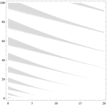
Figure 1: Instability region (shaded area) in the parametric space of the model (17), namely, in terms of values of $(\omega/\omega_{d})^{2}$ (horizontal axis) versus $(\omega_{0}/\omega_{d})^{2}$. The values reported on the axes are in dimensionless units.

In the relevant system the coupling between the oscillators is oscillatory, time-dependent and quadratic. In the Wigner representation, the Hamiltonian of the system is

$$H_{\rm S}=\frac{p_{1}^{2}}{2m}+\frac{p_{2}^{2}}{2m}+\frac{m\omega^{2}}{2}\left(q_{1}^{2}+q_{2}^{2}\right)+\frac{m\tilde{\omega}^{2}(t)}{2}\left(q_{2}-q_{1}\right)^{2}\;,$$ (17)

where $\omega$ is the proper frequency of the oscillators, $\omega=\sqrt{K/m}$, and $\tilde{\omega}(t)$ is the time-dependent frequency of the coupling between the oscillators

$$\tilde{\omega}(t)\equiv\sqrt{\tilde{K}(t)/m}=\omega_{0}\sin\left(\omega_{d}t\right)\;.$$ (18)

Here $p_{1}$ and $p_{2}$ are the momenta of the oscillators, $m$ is the mass of both oscillators, $q_{1}$ and $q_{2}$ are the displacement of the oscillators from their equilibrium positions, $K$ is the spring constant of both oscillators, $\omega_{0}$ is the amplitude frequency of the coupling, $\omega_{d}$ is the driving frequency and $\tilde{K}(t)$ is the coupling function between the oscillators.

In Refs. EntangHighT and linearquantum analytical solutions to similar models have been found. However, our system differs in the time dependence of the coupling between the oscillators. On a classical level our model can be treated in terms of the Mathieu functions and using the Floquet theorem Floquet . Using the notation defined in Appendix B (and assuming $\omega_{c}\equiv\omega_{d}$, where $\omega_{c}$ is the frequency characterizing the spectral density of the bath introduced in Sec. III.1), we obtain the following equations of motion

$$\frac{d^{2}Q_{1}^{\prime}}{dt^{\prime 2}}+\frac{\omega^{2}}{\omega_{d}^{2}}Q_{1}^{\prime}=0\;,$$ (19)

$$\frac{d^{2}Q_{2}^{\prime}}{dt^{\prime 2}}+\left[\frac{\omega^{2}+\omega_{0}^{2}}{\omega_{d}^{2}}-\frac{\omega_{0}^{2}}{\omega_{d}^{2}}\cos{(2t^{\prime})}\right]Q_{2}^{\prime}=0\;,$$ (20)

where $Q_{1}^{\prime}=(q_{1}^{\prime}+q_{2}^{\prime})/\sqrt{2}$ and $Q_{2}^{\prime}=(q_{1}^{\prime}-q_{2}^{\prime})/\sqrt{2}$ are the dimensionless center-of-mass and relative displacement coordinates, respectively. While the solution of Eq. (19) is simply a linear combination of sine and cosine functions, Eq. (20) is the Mathieu equation and possesses more complex features. In particular, for certain values of its parameters, it develops dynamical instabilities, see Fig. 1. Such parameters values must be avoided when doing the numerical simulations in the quantum case.

III.1 Ohmic bath

In order to represent dissipative effects, the relevant system described by the Hamiltonian $H_{\rm S}$ was coupled, via a bilinear coupling, to a bath of $N$ independent harmonic oscillators with an Ohmic spectral density leggett . The total Hamiltonian is

$$H^{\rm NB}=H_{\rm S}+H_{\rm B}+H_{\rm SB}$$ (21)

where

$$H_{\rm B} = \sum_{j=1}^{N}\left(\frac{P_{j}^{2}}{2m_{j}}+\frac{1}{2}m_{j}\Omega_{j}^{2}R_{j}^{2}\right)\;,$$ (22)

$$H_{\rm SB} = -\sum_{\alpha=1}^{2}\sum_{j=1}^{N}q_{\alpha}c_{j}R_{j}\;.$$ (23)

The parameters in Eqs. (22) and (23) are defined as

$$\Omega_{j} = -\omega_{c}\ln{\left(1-j\frac{\bar{\omega}_{0}}{\omega_{c}}\right)}$$ (24)

$$\bar{\omega}_{0} = \frac{\omega_{c}}{N}\left[1-\exp{\left(-\frac{\omega_{\rm max}}{\omega_{c}}\right)}\right]$$ (25)

$$c_{j} = \sqrt{\xi\hbar\bar{\omega}_{0}m_{j}}\Omega_{j}\;.$$ (26)

The frequency $\omega_{\rm max}$ in Eq. (25) is a cut-off frequency used in the numerical representation of the spectral density. The value of $\omega_{\rm max}$ used in the calculations reported in this work is given in Sec. IV. Each oscillator in the bath has a different frequency, $\Omega_{j}$. The definition of $\Omega_{j}$, $\bar{\omega}_{0}$ and $c_{j}$ is chosen in such a way to represent an infinite bath of oscillators with Ohmic spectral density leggett in terms of discrete mode of oscillations makri ; linear1 ; linear2 . The parameters $\xi$ and $\omega_{c}$ characterize the spectral density of the bath. The Kondo parameter, $\xi$, is a measure of the strength of the coupling between the relevant system and the bath.

Figure 2: Variance of the position and momentum coordinate of each normal mode, where the relevant system is attached to a harmonic bath. The shaded square, circle, triangle and diamond points represent the variances of $R_{1}$, $R_{2}$, $P_{1}$ and $P_{2}$ respectively. Solid lines, connecting the numerically calculated points, have been drawn to guide the eye. Dimensionless parameters used in this simulation: $m=1.0$, $K=1.25$, $\omega_{0}=2.50$, $\omega_{d}=0.45$, $\xi=0.007$ and $T_{\rm ext}=1.0$. The values reported on the axes are also in dimensionless units.

III.2 NHC representation of the bath

We adopted a second technique to represent the dissipative environment in which the relevant driven system is embedded. In particular, we considered a single oscillator bilinearly coupled to the relevant system and we thermalized it by means of a Nosé-Hoover Chain nhc ; nonHamTherm . Such a technique (and similar ones dlamini ; b3 ) allows one to reduce drastically the computational time by representing the thermal environment with a minimal number of degrees of freedom. In this case, the total Hamiltonian is

$$H^{\rm NHC} = H_{\rm S}+H_{\rm B}^{1}+H_{\rm SB}^{1}+H^{\rm TH}\;,$$ (27)

$$H_{\rm B}^{1} = \frac{P_{1}^{2}}{2m_{1}}+\frac{1}{2}M\Omega_{1}^{2}R_{1}^{2}\;,$$ (28)

$$H_{\rm SB}^{1} = -c_{1}R_{1}\left(q_{1}+q_{2}\right)\;,$$ (29)

$$H^{\rm TH} = \frac{P_{\eta_{1}}^{2}}{2m_{\eta_{1}}}+\frac{P_{\eta_{2}}^{2}}{2m_{\eta_{2}}}+k_{B}T_{\rm ext}\eta_{1}+k_{B}T_{\rm ext}\eta_{2}\;.$$ (30)

Here $P_{1}$ and $R_{1}$ are the phase space variables of the bath oscillator having mass $m_{1}$ and frequency $\Omega_{1}$. The bath and driven system are bilinearly coupled. The fictitious Nosé variables are indicated by $\eta_{1}$ and $\eta_{2}$ while $P_{\eta_{1}}$ and $P_{\eta_{2}}$ are their associate momenta. The fictitious Nosé variables have masses $m_{\eta_{1}}$ and $m_{\eta_{2}}$, respectively. The symbol $k_{B}$ denotes the Boltzmann constant while $T_{\rm ext}$ indicates the absolute temperature of the bath. As explained with more detail in Appendix A, the coupling to the fictitious thermostat variables $(\eta_{1},\eta_{2},p_{\eta_{1}},p_{\eta_{2}})$ is realized through the non-Hamiltonian equation of motion. In the classical case, such equations are written in compact form in Eq. (15) or in explicit form in Eqs. (46-51). In the quantum case, the coupling is given through Eq. (16). The quantum-classical approximation of Eq. (16), which suppresses the spurious quantum effects over the fictitious NHC variables, is instead given in Eq. (55). Equation (55) is the one used for the NHC representation of the bath in this work.

Figure 3: Variance of the position coordinate of normal mode 2, $R_{2}$, where the relevant system is attached to a harmonic bath. A horizontal line at $\langle(\Delta R_{2})^{2}\rangle$=0.5 shows the theoretical threshold value for squeezed state generation. The inset shows the short time simulation of the variance of $R_{2}$, represented by solid circles. A solid line, connecting the numerically calculated points, has been drawn to guide the eye. Dimensionless parameters used in this simulation: $m=1.0$, $K=1.25$, $\omega_{0}=2.50$, $\omega_{d}=0.45$, $\xi=0.007$ and $T_{\rm ext}=1.0$. The values reported on the axes are also in dimensionless units.

IV Simulation details

The algorithm used to integrate the equations of motion in all our simulations is based on the symmetric Trotter factorization of the propagator reversibleintegrators ; reverse_int . When we considered the NHC thermostat to represent the thermal bath, we also incorporated the Yoshida scheme yoshida with three iterations and a multiple time-step procedure with three iterations, following the approach of Ref. reversibleintegrators . In the simulations, we set as initial conditions for the NHC variables $\eta_{1}=0$, $\eta_{2}=0$, $p_{\eta_{1}}=0$ and $p_{\eta_{2}}=1.0$.

At $t=0$ it is assumed that the system is at thermal equilibrium with no time-dependent driving. The driving acts for $t>0$. In this case, the Wigner function of the total system is positive definite and can be represented as a collection of points that are propagated according to Eq. (6), when the bath is represented by means of $N$ oscillators with an Ohmic spectral density, or according to Eq. (16), when using the NHC bath.

In order to sample the initial configuration of the relevant system, it is useful to introduce normal coordinates Goldstein :

$$\tilde{q}_{1} = \frac{1}{\sqrt{2}}\left(q_{1}+q_{2}\right)\;,$$ (31)

$$\tilde{q}_{2} = \frac{1}{\sqrt{2}}\left(q_{1}-q_{2}\right)\;,$$ (32)

$$\tilde{p}_{1} = \frac{1}{\sqrt{2}}\left(p_{1}+p_{2}\right)\;,$$ (33)

$$\tilde{p}_{2} = \frac{1}{\sqrt{2}}\left(p_{1}-p_{2}\right)\;,$$ (34)

so that the Hamiltonian $H_{\rm S}$ in Eq. (17) can be written as

$$H^{\rm NM} = \sum_{k=1}^{2}\left(\frac{\tilde{p}_{k}^{2}}{2m}+\frac{1}{2}m\omega_{k}^{2}\tilde{q}_{k}^{2}\right)\;,$$ (35)

where $\omega_{k}$ ($k=1,2$) are the normal mode frequencies. The symbol $\tilde{q}_{1}$ represents the motion of the centre of mass of the system, while $\tilde{q}_{2}$ represents the relative displacements of the oscillators. The normal mode frequencies of each mode are

$$\omega_{1} = \sqrt{\frac{K}{m}}\;,$$ (36)

$$\omega_{2}(t) = \sqrt{\frac{K+2\tilde{K}(t)}{m}}\;.$$ (37)

The initial conditions of the system are sampled from the Wigner function DistFunctions :

$$W_{\rm S}=\prod_{k=1}^{2}\frac{1}{\pi\hbar}\tanh\left(\frac{\hbar\omega_{k}}{2}\beta\right)\exp\left(-\frac{\tilde{p}_{k}^{2}}{2\sigma_{\tilde{p}_{k}}^{2}}\right)\exp\left(-\frac{\tilde{q}_{k}^{2}}{2\sigma_{\tilde{q}_{k}}^{2}}\right)$$ (38)

where

$$\sigma_{\tilde{p}_{k}} = \left[\frac{2}{\hbar m\omega_{k}}\tanh\left(\frac{\hbar\omega_{k}}{2}\beta\right)\right]^{-\frac{1}{2}}\;,$$ (39)

$$\sigma_{\tilde{q}_{k}} = \left[\frac{2m\omega_{k}}{\hbar}\tanh\left(\frac{\hbar\omega_{k}}{2}\beta\right)\right]^{-\frac{1}{2}}\;.$$ (40)

In the high temperature limit $\left(T\rightarrow\infty,\beta\rightarrow 0\right)$, the Wigner distribution function in Eq. (38) reduces to the classical canonical distribution function, $Z^{-1}\exp[-\beta H_{\rm S}]$. Hence, simply by changing the sampling of the initial conditions of the system, we can study the difference between the classical and the quantum behavior of the system.

At $t=0$, the Ohmic bath is also assumed to be at thermal equilibrium with initial Wigner function equal to

$$W_{\rm B}=\prod_{k=1}^{N}\frac{1}{\pi\hbar}\tanh\left(\frac{\hbar\Omega_{k}}{2}\beta\right)\exp\left(-\frac{P_{k}^{2}}{2\sigma_{P_{k}}^{2}}\right)\exp\left(-\frac{R_{k}^{2}}{2\sigma_{R_{k}}^{2}}\right)$$ (41)

where

$$\sigma_{P_{k}} = \left[\frac{2}{\hbar m\Omega_{k}}\tanh\left(\frac{\hbar\Omega_{k}}{2}\beta\right)\right]^{-\frac{1}{2}}$$ (42)

$$\sigma_{R_{k}} = \left[\frac{2m\Omega_{k}}{\hbar}\tanh\left(\frac{\hbar\Omega_{k}}{2}\beta\right)\right]^{-\frac{1}{2}}\;.$$ (43)

So that the initial Wigner function for the total system is $W=W_{S}\times W_{\rm B}$.

When using the NHC representation of the bath, $W_{\rm B}$ in Eq. (41) reduces to $W_{\rm B}^{1}$ (which is obtained considering $N=1$) while the initial condition of the NHC fictitious variables are taken as $\prod_{n=1}^{2}\delta(p_{\eta_{n}}-p_{\eta_{n}}^{0})\delta(\eta_{n}-\eta_{n}^{0})$, where $(\eta_{n}^{0},p_{\eta_{n}}^{0})$, $n=1,2$, are some arbitrary fixed values. In such a case, the total initial Wigner function is $W=W_{\rm S}\times W_{\rm B}^{1}\times\prod_{n=1}^{2}\delta(p_{\eta_{n}}-p_{\eta_{n}}^{0})\delta(\eta_{n}-\eta_{n}^{0})$.

Considering two arbitrary quantum operators, $\hat{a}$ and $\hat{b}$, satisfying the commutation relation $[\hat{a},\hat{b}]=i\hat{c}$, it is known that there is a squeezed state if QOptics

$$\left<\left(\Delta a_{\rm W}\right)^{2}\right><\frac{1}{2}\left|\left<c_{\rm W}\right>\right|\ \mathrm{or}\ \left<\left(\Delta b_{\rm W}\right)^{2}\right><\frac{1}{2}\left|\left<c_{\rm W}\right>\right|\;,$$ (44)

where $a_{\rm W}$, $b_{\rm W}$ and $c_{\rm W}$ are the Wigner representation of $\hat{a}$, $\hat{b}$ and $\hat{c}$, respectively, and $\Delta a_{\rm W}=a_{W}-\langle a_{\rm W}\rangle$. In the case the normal mode coordinates, Eqs. (31-34), their commutation relations are $\left[\hat{\tilde{q}}_{j},\hat{\tilde{p}}_{k}\right]=i\hbar\delta_{jk}$, $j,k=1,2$. In dimensionless coordinates, the conditions of squeezing can be written as

$$\left<\left(\Delta\tilde{q}_{k}\right)^{2}\right><\frac{1}{2}\quad \mathrm{or} \quad\left<\left(\Delta\tilde{p}_{k}\right)^{2}\right><\frac{1}{2}\;.$$ (45)

Equation (45) provides a threshold for state squeezing. Upon defining $\chi_{k}=\tilde{q}_{k}^{2}-\langle\tilde{q}_{k}\rangle^{2}$ or $\chi_{k}=\tilde{p}_{k}^{2}-\langle\tilde{p}_{k}\rangle^{2}$ for $k=1,2$, one can use Eq. (2) in order to assess state squeezing. The squeezed states can be visualized upon constructing the marginal distribution functions of each normal mode from the numerical evolution of the total Wigner function.

V Numerical Results

In all simulations we considered an integration time step $dt=0.01$, a number of molecular dynamics steps $N_{\rm S}=25000$, and a number of Monte Carlo steps $N_{\rm MC}=10000$. Unless stated otherwise, the results are reported in dimensionless coordinates and scaled units. We performed simulations considering three different cases. The first concerns the study of the driven oscillators without the coupling to an external bath. The second deals with the driven oscillators bi-linearly coupled to an Ohmic bath. The third concerns the driven oscillators coupled to a dissipative bath constituted by a single harmonic oscillator thermalized though a Nosé-Hoover Chain. We did not find any appreciable numerical difference between the results obtained with the Ohmic bath or with the single harmonic oscillator thermalized though a NHC thermostat.

In order to check our calculation scheme, we ran a series of simulations without taking into account dissipative effects. Instead, we focused on the dynamics of the two coupled oscillators with the Hamiltonian given in Eq. (17). The stability of the numerical algorithm was tested by calculating the average value of the energy when considering $\tilde{\omega}=\omega_{0}$ (which amounts to switching off the time-dependent coupling) in Eq. (17). Such an average value was found to be conserved in one part over ten thousand. Upon reintroducing the time-dependent frequency in Eq. (17), we also verified that a squeezed state is generated. Starting from a thermal state, the variance of the position and momentum of each normal mode coordinate was calculated. The variance of the position of normal mode 2 was found to be below the threshold for squeezing while the variance of the momentum of normal mode 2 increases simultaneously (in agreement with the Heisenberg uncertainty principle). This indicated that a squeezed state for the position coordinate of normal mode 2 had been generated.

Figure 4: Variance of normal mode coordinate $R_{2}$, with three different temperatures of the bath. The square, circle, and triangle points are for temperatures of the bath 1.0, 1.037 and 1.06, respectively. The inset shows the same curves in the long-time region in order to better appreciate their differences. Solid lines, connecting the numerically obtained points, have been drawn to guide the eye. Moreover, a horizontal line at $\langle(\Delta R_{2})^{2}\rangle$=0.5 shows the theoretical threshold value for squeezed state generation. Dimensionless parameters used in this simulation: $m=1.0$, $K=1.25$, $\omega_{0}=2.50$, $\omega_{d}=0.45$, and $\xi=0.007$. The values reported on the axes are also in dimensionless units.

In order to account for dissipative effects and study the influence of a thermal bath on squeezed state generation, we used two methods that, as expected dlamini ; b3 , provided numerically indistinguishable results. In the first approach, we used a bath of $N=200$ harmonic oscillators, bi-linearly coupled to the system of driven oscillators. It has been shown that such a discrete representation of the Ohmic bath is in agreement with linear response theory linear1 ; linear2 . The Hamiltonian of this system is given in Eq. (21). In the second approach, we represented the bath by means of a single oscillator coupled to a NHC thermostat. In this second case, the Hamiltonian of the system is given in Eq. (27). The values of the fictitious masses $m_{\eta_{1}}$ and $m_{\eta_{2}}$ control the dynamics of the thermostat, which in turn simulates the thermal bath. Such masses are tunable parameters that can be adjusted in order to obtain an optimal agreement between the calculations with $N=200$ and no thermostat and those with $N=1$ with the thermostat. In the calculations reported in this work, we set $m_{\eta_{1}}=m_{\eta_{2}}=1.0$ (in dimensionless units). We also observed that, for the model studied, the agreement between the results (obtained by means of the two different representations of the bath) is achieved within the range of values $0.96\leq m_{\eta_{1}}=m_{\eta_{2}}\leq 1.04$ of the fictitious masses.

All calculations were performed using $\omega_{c}=1.0$ and $\omega_{\rm max}=3.0$. Both weak and strong coupling strengths to the bath ($\xi=0.007,0.3$) were studied. We observed that the coupling strengths influenced the behavior of normal mode 1 while normal mode 2 remained almost invariant. Figure 2 shows the variance of each normal mode coordinate. The variance of the coordinates of normal mode 1 maintain a constant value even when the driving is switched on between the oscillators. However, we observe a decrease in the variance of the position and an increase in the variance of the momentum of normal mode 2, respectively. This arises from the form of the normal mode frequencies in Eqs. (36) and (37): only the frequency of normal mode 2 is time-dependent, while the frequency of normal mode 1 has a constant value. In Fig. 3 we have plotted the theoretical threshold for squeezing as defined in Eq. (45). The variance of the position of normal mode 2 is clearly below such a threshold. This shows that the driven oscillators can make a transition from a thermal to a squeezed state, as expected. The inset in Fig. 3 shows the dynamics over a short time interval of the variance of the position of normal mode 2. The variance goes below the squeezing threshold after a time interval $\Delta t=3.2$ and remains below such a threshold for the rest of its time evolution. We can conclude that the generation of a squeezed state is fast in comparison to the natural dynamics of the system. At time $t=0$, the marginal distribution functions of both normal modes are symmetrical and have a circular uncertainty domain schleich . After the driving is turned on, the marginal distribution function of normal mode 1 maintains its initial features, while the marginal distribution function of normal mode 2 becomes asymmetrical with an elliptical uncertainty domain.

We also studied the influence of the temperature on the degree of squeezing of the normal modes. In particular, we have performed simulations for various values of the temperature ranging from 0.95 to 1.06 (and used an increment of 0.01). In Figure 4, the results of three different bath temperatures ($T_{\rm ext}$=1.0, 1.037, and 1.06) are shown. The value of $T_{\rm ext}$=1.037 provides a reliable estimate of the threshold temperature for the creation of squeezed states in our model, i.e., above this temperature no squeezing is produced by the time-dependent dynamics. As a matter of fact, we verified that for $T_{\rm ext}$=1.038 we did not observe any squeezing. Below $T_{\rm ext}$=1.037, for the various temperatures calculated, we have always observed the creation of squeezed states in our model.

VI Conclusions and perspectives

We studied the generation of squeezed states induced by time-dependent quadratic coupling between two harmonic oscillators embedded in a dissipative environment. The latter was represented in two different ways that provided numerically indistinguishable results. In one approach, we used a bath of $N=200$ harmonic oscillators with an Ohmic spectral density; in the other approach, we used a single harmonic oscillator whose temperature was controlled through a Nosé-Hoover Chain non-Hamiltonian thermostat. The quantum equations of motion were mapped onto a classical-like formalism through the Wigner representation and integrated numerically by means of standard molecular dynamics techniques. The systems studied are relevant in order to model the dynamics of molecular phonons (for example) in condensed matter.

Upon varying the controlled temperature of the bath in our calculations, we studied the effect of thermal disorder on the generation of squeezing. It was found that there is a threshold temperature of the bath below which squeezing is still present. In dimensionless coordinates, this temperature is $T_{\rm ext}=1.037$. The non-Hamiltonian thermostat is defined in terms of two free parameters, $m_{\eta_{1}}$ and $m_{\eta_{2}}$, which play the role of fictitious masses. We observed that, for the model studied, the agreement between the results (obtained by means of the two different representations of the bath) is achieved within the range of values $0.96\leq m_{\eta_{1}}=m_{\eta_{2}}\leq 1.04$.

If we assume a value of the frequency $\omega_{c}=3.93\times 10^{13}$ Hz we can convert to dimensionful coordinates and find that such a temperature has the value $T_{\rm ext}=311.13$ K. According to this, the quantum of excitation $\hbar\omega_{c}$ assumes the value of 4.14 $\times 10^{-21}$ J, which is exactly equal to the value of $k_{B}T$ at room temperature ($T_{\rm ext}$=300 K corresponding to $T_{\rm ext}=1.0$ in dimensionless coordinates). With the above value of $\omega_{c}$, we found two interesting results. One is that the time spanned by the simulated trajectories is of the same order of magnitude as that of molecular oscillations ($\approx 10^{12}$ s). The second is that the frequency of vibration of the relevant oscillators is of the order of the terahertz, as it is expected for molecular functional dynamics in biological systems zhang . Hence, our numerical study supports the possibility of having observable quantum effects at temperatures that are relevant for biological functions. As suggested by various authors poc09 ; EntangHighT ; EntangHighT2 ; gue12 ; pachon , such a counterintuitive occurrence is made possible by the non-equilibrium conditions arising in the dynamics of coupled molecular systems. In this work and elsewhere poc09 ; EntangHighT ; EntangHighT2 ; gue12 ; pachon , such complex situations have been modeled through phononic modes with a time-dependent coupling. However, through a suitable modification of the Wigner trajectory method, the techniques illustrated in this paper promise a somewhat straightforward extension to non-harmonic couplings and non-Markovian dynamics.

Appendix A Wigner NHC equations of motion

Let us consider the Hamiltonian in Eq. (7) and the antisymmetric matrix in Eq. (14). The non-Hamiltonian equations on motion (15) are written explicitly as

$$\dot{r} = \frac{p}{m}\;,$$ (46)

$$\dot{\eta_{1}} = \frac{p_{\eta_{1}}}{m_{\eta_{1}}}\;,$$ (47)

$$\dot{\eta_{2}} = \frac{p_{\eta_{2}}}{m_{\eta_{2}}}\;,$$ (48)

$$\dot{p} = -\frac{\partial V}{\partial r}-\frac{p_{\eta_{1}}}{m_{\eta_{1}}}p\;,$$ (49)

$$\dot{p}_{\eta_{1}} = \frac{p^{2}}{m}-gk_{B}T-\frac{p_{\eta_{2}}}{m_{\eta_{2}}}p_{\eta_{1}}\;,$$ (50)

$$\dot{p}_{\eta_{2}} = \frac{p_{\eta_{1}}^{2}}{m}-k_{B}T\;.$$ (51)

The Liouville operator for NHC dynamics is

$$L^{\rm NHC}={\cal B}_{ij}^{\rm NHC}\frac{\partial H^{\rm NHC}}{\partial x_{i}}\frac{\partial}{\partial x_{i}}$$

$$\qquad\ \ \,=\frac{p}{m}\frac{\partial}{\partial r}+\frac{p_{\eta_{1}}}{m_{\eta_{1}}}\frac{\partial}{\partial\eta_{1}}+\frac{p_{\eta_{2}}}{m_{\eta_{2}}}\frac{\partial}{\partial\eta_{2}}$$

$$\qquad\ \ \ +\left(-\frac{\partial V}{\partial r}-\frac{p_{\eta_{1}}}{m_{\eta_{1}}}p\right)\frac{\partial}{\partial p}$$

$$\qquad\ \ \ +\left(\frac{p^{2}}{m}-gk_{B}T\right)\frac{\partial}{\partial p_{\eta}}$$

$$\qquad\ \ \ +\left(\frac{p_{\eta_{1}}^{2}}{m}-k_{B}T\right)\frac{\partial}{\partial p_{\eta_{2}}}\;.$$ (52)

The above equations allow one to define NHC dynamics in classical phase space. The coupling between the thermostat momentum $p_{\eta_{1}}$ and the physical coordinates $p$ is not realized through the extended Hamiltonian in Eq. (7). Instead, it is achieved through Eq. (49). Under the assumption of ergodicity, it can be proven that the NHC equations of motion (46-51) generate the canonical distribution function for the physical coordinates $(r,p)$ nhc ; nheom .

As originally explained in Ref. nonHamTherm , the matrix form of the generalized Wigner bracket given in Eq. 16 can be used to define NHC equations of motion in quantum phase space. Defining the phase space compressibility as

$$\kappa=(\partial_{j}B_{ji}^{\rm NHC})\partial_{i}H^{\rm NHC}\;,$$ (53)

the Wigner NHC equation can be written as

$$\partial_{t}W = -iL^{\rm NHC}W-\kappa W+\sum_{n=3,5,7,\ldots}\frac{1}{n!}\left(\frac{i\hbar}{2}\right)^{n-1}H^{\rm NHC}\left[\overleftarrow{\partial_{i}}{\cal B}_{ij}^{\rm NHC}\overrightarrow{\partial_{j}}+\overleftarrow{\partial_{i}}(\partial_{j}{\cal B}_{ij}^{\rm N})\right]^{n}f_{W},$$ (54)

where the Nosé Liouville operator is defined as in Eq. (52) and $W=W(r,p,\eta_{1},\eta_{2},p_{\eta_{1}},p_{\eta_{2}},t)$ is the Wigner distribution function in the extended NHC quantum phase space. To zeroth order in $\hbar$ the Nosé-Wigner equations of motion coincide with the classical equations of motion. Higher powers of $\hbar$ provide the quantum corrections to the dynamics. The quantum correction terms were considered in more detail in Ref. nonHamTherm . However, one is not really interested in the quantum behavior of the fictitious variables: they are there only to enforce the canonical distribution and represent a thermal environment. Moreover, the mass $m_{\eta_{1}}$ is typically taken to be much greater than $m$ in order to not modify the dynamical properties of the system. As a result, one finds a small expansion parameter $\mu=\sqrt{m/m_{\eta_{1}}}<<1$ that can be used to take the classical limit over the $(\eta_{1},\eta_{2},p_{\eta_{1}},p_{\eta_{2}})$ fictitious variables. In such a way, in place of the full quantum equation (54) one obtains

$$\partial_{t}W = -\left(iL^{\rm NHC}+\kappa\right)W+\sum_{n=3,5,7,\ldots}\frac{1}{n!}\left(\frac{i\hbar}{2}\right)^{n-1}\!V\left(\overleftarrow{\partial}_{r}\overrightarrow{\partial_{p}}\right)^{n}W.$$ (55)

Equation (55) defines a quantum-classical NHC dynamics according to which the $(r,p)$ coordinates are evolved quantum-mechanically while the $(\eta_{1},\eta_{2},p_{\eta_{1}},p_{\eta_{2}})$ are evolved classically. As proven in Ref. nonHamTherm , the weak coupling between the two sets of coordinates generates a canonical distribution function to zero order in $\hbar$.

Appendix B Converting equations to dimensionless form

It is convenient to introduce the following dimensionless variables:

$$q^{\prime}_{i}=q_{i}\sqrt{\frac{m\omega_{c}}{\hbar}},\ p^{\prime}_{i}=\frac{p_{i}}{\sqrt{mE_{c}}},$$ (56)

$$R^{\prime}_{j}=R_{j}\sqrt{\frac{m_{j}\omega_{c}}{\hbar}},\ P^{\prime}_{j}=\frac{P_{j}}{\sqrt{m_{j}E_{c}}},$$ (57)

$$R^{\prime}_{1}=R_{1}\sqrt{\frac{m_{1}\omega_{c}}{\hbar}},\ P^{\prime}_{1}=\frac{P_{1}}{\sqrt{m_{1}E_{c}}},$$ (58)

$$P^{\prime}_{\eta_{1}}=\frac{P_{\eta_{1}}}{\sqrt{m_{\eta_{1}}E_{c}}},\ P^{\prime}_{\eta_{2}}=\frac{P_{\eta_{2}}}{\sqrt{m_{\eta_{2}}E_{c}}},$$ (59)

$$t^{\prime}=\omega_{c}t,\ H^{\prime}=\frac{H}{E_{c}},\ T^{\prime}=\frac{k_{B}T}{E_{c}},$$ (60)

and

$$\tilde{\omega}^{\prime}(t^{\prime})=\frac{\tilde{\omega}(t)}{\omega_{c}}=\omega_{0}^{\prime}\sin\left(\omega_{d}^{\prime}t^{\prime}\right),$$ (61)

$$\omega^{\prime}=\frac{\omega}{\omega_{c}},\ \omega_{0}^{\prime}=\frac{\omega_{0}}{\omega_{c}},\ \omega_{d}^{\prime}=\frac{\omega_{d}}{\omega_{c}},$$ (62)

$$\bar{\omega}_{0}^{\prime}=\frac{\bar{\omega}_{0}}{\omega_{c}}=\frac{1}{N}\left[1-\exp{(-\omega_{\rm max}^{\prime})}\right],$$ (63)

$$\Omega_{j}^{\prime}=\frac{\Omega_{j}}{\omega_{c}}=-\ln{\left(1-j\bar{\omega}_{0}^{\prime}\right)}\;,$$ (64)

$$\omega_{\rm max}^{\prime}=\frac{\omega_{\rm max}}{\omega_{c}},\ \Omega_{1}^{\prime}=\frac{\Omega_{1}}{\omega_{c}},$$ (65)

and

$$c_{j}^{\prime}=\frac{c_{j}}{\omega_{c}\sqrt{mm_{j}\Omega_{j}\omega_{c}}}=\sqrt{\frac{\xi\hbar\bar{\omega}_{0}^{\prime}\Omega_{j}^{\prime}}{m\omega_{c}}},$$ (66)

$$c_{1}^{\prime}=\frac{c_{1}}{\omega_{c}\sqrt{mm_{1}\Omega_{1}\omega_{c}}}=\sqrt{\frac{\xi\hbar\bar{\omega}_{0}^{\prime}\Omega_{1}^{\prime}}{m\omega_{c}}},$$ (67)

where $E_{c}=\hbar\omega_{c}$ and the indices $i$ and $j$ run from 1 to 2 and from 1 to $N$, respectively. Also, the Hamiltonian $H$ and temperature $T$ can carry any subscripts as prescribed by a model. Unless stated otherwise, all these definitions are valid throughout the paper. Using them, the main equations of the above-mentioned three models can be written as follows.

The dimensionless Hamiltonian of the model in Eq. (17) takes the form

$$H_{\rm S}^{\prime}=\frac{p^{\prime 2}_{1}}{2}+\frac{p^{\prime 2}_{2}}{2}+\frac{\omega^{\prime 2}}{2}\left(q_{1}^{\prime 2}+q_{2}^{\prime 2}\right)+\frac{\tilde{\omega}^{\prime 2}(t)}{2}\left(q_{2}^{\prime}-q_{1}^{\prime}\right)^{2},$$ (68)

and the equations of motion for the dimensionless phase-space coordinates $\left(q_{1}^{\prime},q_{2}^{\prime},p_{1}^{\prime},p_{2}^{\prime}\right)$ can be written as

$$\frac{dq_{1}^{\prime}}{dt^{\prime}} = p_{1}^{\prime},$$ (69)

$$\frac{dq_{2}^{\prime}}{dt^{\prime}} = p_{2}^{\prime},$$ (70)

$$\frac{dp_{1}^{\prime}}{dt^{\prime}} = -\omega^{\prime 2}q_{1}^{\prime}+\tilde{\omega}^{\prime 2}(t^{\prime})\left(q_{2}^{\prime}-q_{1}^{\prime}\right),$$ (71)

$$\frac{dp_{2}^{\prime}}{dt^{\prime}} = -\omega^{\prime 2}q_{2}^{\prime}-\tilde{\omega}^{\prime 2}(t^{\prime})\left(q_{2}^{\prime}-q_{1}^{\prime}\right).$$ (72)

As long as for this model the value $\omega_{c}$ does not appear in the Hamiltonian or elsewhere, for actual computations one could naturally assume $\omega_{c}\equiv\kappa\omega_{d}$, where $\kappa$ is any natural number, for example.

The dimensionless Hamiltonian of the model defined in Eqs. (21-23) can be written as

$$H_{\rm NB}^{\prime} = \frac{p_{1}^{\prime 2}}{2}+\frac{p_{2}^{\prime 2}}{2}+\frac{\omega^{\prime 2}}{2}q_{1}^{\prime 2}+\frac{\omega^{\prime 2}}{2}q_{2}^{\prime 2}$$ (73)

$$+ \frac{\tilde{\omega}^{\prime 2}(t)}{2}\left(q_{2}^{\prime 2}-q_{1}^{\prime 2}\right)+\sum_{j=1}^{N}\left(\frac{P_{j}^{\prime 2}}{2}+\frac{1}{2}\Omega_{j}^{\prime 2}R_{j}^{\prime 2}\right)$$

$$- \left(q_{1}^{\prime}+q_{2}^{\prime}\right)\sum_{j=1}^{N}c_{j}^{\prime}R_{j}^{\prime},$$

and the equations of motion for the dimensionless phase-space coordinates $\left(q_{1}^{\prime},q_{2}^{\prime},R_{j}^{\prime},p_{1}^{\prime},p_{2}^{\prime},P_{j}^{\prime}\right)$ are

$$\frac{dq_{1}^{\prime}}{dt^{\prime}} = p_{1}^{\prime},$$ (74)

$$\frac{dq_{2}^{\prime}}{dt^{\prime}} = p_{2}^{\prime},$$ (75)

$$\frac{dR_{j}^{\prime}}{dt^{\prime}} = P_{j}^{\prime},$$ (76)

$$\frac{dp_{1}^{\prime}}{dt^{\prime}} = -\omega^{\prime 2}q_{1}^{\prime}+\tilde{\omega}^{\prime 2}(t^{\prime})\left(q_{2}^{\prime}-q_{1}^{\prime}\right)+\sum_{j=1}^{N}c_{j}^{\prime}R_{j}^{\prime},$$ (77)

$$\frac{dp_{2}^{\prime}}{dt^{\prime}} = -\omega^{\prime 2}q_{2}^{\prime}-\tilde{\omega}^{\prime 2}(t)\left(q_{2}^{\prime}-q_{1}^{\prime}\right)+\sum_{j=1}^{N}c_{j}^{\prime}R_{j}^{\prime},$$ (78)

$$\frac{dP_{j}^{\prime}}{dt^{\prime}} = -\Omega^{\prime 2}_{j}R_{j}^{\prime}+c_{j}^{\prime}\left(q_{1}^{\prime}+q_{2}^{\prime}\right).$$ (79)

Finally, the dimensionless Hamiltonian of the NHC model (27) can be written as

$$H_{\rm NHC}^{\prime} = \frac{p_{1}^{\prime 2}}{2}+\frac{p_{2}^{\prime 2}}{2}+\frac{\omega^{\prime 2}}{2}q_{1}^{\prime 2}+\frac{\omega^{\prime 2}}{2}q_{2}^{\prime 2}$$ (80)

$$+ \frac{\tilde{\omega}^{\prime 2}(t)}{2}\left(q_{2}^{\prime}-q_{1}^{\prime}\right)^{2}+\frac{P_{1}^{\prime 2}}{2}+\frac{\omega_{1}^{\prime 2}}{2}R_{1}^{\prime 2}$$

$$- c_{1}^{\prime}R_{1}^{\prime}\left(q_{1}^{\prime}+q_{2}^{\prime}\right)+\frac{P_{\eta_{1}}^{\prime 2}}{2}+\frac{P_{\eta_{2}}^{\prime 2}}{2}$$

$$+ gT_{\rm ext}^{\prime}\eta_{1}+T_{\rm ext}^{\prime}\eta_{2},$$

and the equations of motion for the dimensionless phase-space coordinates $\left(q_{1}^{\prime},q_{2}^{\prime},R_{1}^{\prime},\eta_{1},\eta_{2},p_{1}^{\prime},p_{2}^{\prime},P_{1}^{\prime},P_{\eta_{1}}^{\prime},P_{\eta_{2}}^{\prime}\right)$ are

$$\frac{dq_{1}^{\prime}}{dt^{\prime}} = p_{1}^{\prime}\;,$$ (81)

$$\frac{dq_{2}^{\prime}}{dt^{\prime}} = p_{2}^{\prime}\;,$$ (82)

$$\frac{dR_{1}^{\prime}}{dt^{\prime}} = P_{1}^{\prime}\;,$$ (83)

$$\frac{d\eta_{1}}{dt^{\prime}} = P_{\eta_{1}}^{\prime}\;,$$ (84)

$$\frac{d\eta_{2}}{dt^{\prime}} = P_{\eta_{2}}^{\prime}\;,$$ (85)

$$\frac{dp_{1}^{\prime}}{dt^{\prime}} = -\omega^{\prime 2}q_{1}^{\prime}+\tilde{\omega}^{\prime 2}(t^{\prime})\left(q_{2}^{\prime}-q_{1}^{\prime}\right)+c_{1}^{\prime}R_{1}^{\prime}\;,$$ (86)

$$\frac{dp_{2}^{\prime}}{dt^{\prime}} = -\omega^{\prime 2}q_{2}^{\prime}-\tilde{\omega}^{\prime 2}(t)\left(q_{2}^{\prime}-q_{1}^{\prime}\right)+c_{1}^{\prime}R_{1}^{\prime}\;,$$ (87)

$$\frac{dP_{1}^{\prime}}{dt^{\prime}} = -\Omega^{\prime 2}_{j}R_{1}^{\prime}+c_{1}^{\prime}\left(q_{1}^{\prime}+q_{2}^{\prime}\right)\;,$$ (88)

$$\frac{dP_{\eta_{1}}^{\prime}}{dt^{\prime}} = \left(P_{1}^{\prime 2}-gT_{\rm ext}^{\prime}\right)-P_{\eta_{1}}^{\prime}P_{\eta_{2}}^{\prime}\;,$$ (89)

$$\frac{dP_{\eta_{2}}^{\prime}}{dt^{\prime}} = P_{\eta_{1}}^{\prime 2}-T_{\rm ext}^{\prime}\;.$$ (90)

References

- (1) E. Schrödinger, What is Life? Cambridge University Press, Cambridge (2013).
- (2) M. A. Chang and M. Nielsen, Quantum Computation and Quantum Information. Cambridge University Press, Cambridge (2011).
- (3) G. S. Engel, et al., Nature 446, 782-786 (2007).
- (4) E. Collini, et al., Nature 463, 644-647 (2010).
- (5) G. Panitchayangkoon, et al., Proc. Natl Acad. Sci. 108, 20908-20912 (2011).
- (6) G. R. Fleming, S. F. Huelga, and M. B. Plenio, New J. Phys. 13, 115002 pp. 5 (2011).
- (7) H. J. Briegel and S. Popescu, Proc. R. Soc. A 469, 20110290 pp. 9 (2013).
- (8) N. Poccia, A. Ricci, D. Innocenti, and A. Bianconi, Int. J. Molec. Sci. 10, 2084-2106 (2009).
- (9) A. Valletta, et al., J. Superconductivity 10, 383-387 (1997).
- (10) A. W. Chin, A. Datta, F. Caruso, S. F. Huelga, and M. B. Plenio, New J. Phys. 12, 065002 pp. 16 (2010).
- (11) F. Galve, L. A. Pachón and D. Zueco, Phys. Rev. Lett. 105, 180501 pp. 4 (2010).
- (12) F. Galve, G. L. Giorgi, and R. Zambrini, Phys. Rev. A 81, 062117 pp. 10 (2010).
- (13) G. G. Guerreschi, J. Cai, S. Popescu, H. J. Briegel, New J. Phys. 14, 053043 pp. 21 (2012).
- (14) A. F. Estrada and L. A. Pachon, arXiv:1411.3382 [quant-ph] (2014).
- (15) L. Amico, R. Fazio, A. Osterloh, and V. Vedral, Rev. Mod. Phys. 80, 517-576 (2008).
- (16) R. Horodecki, P. Horodecki, M. Horodecki, and K. Horodecki, Rev. Mod. Phys. 81, 865-942 (2009).
- (17) Irreversible Quantum Dynamics, Lecture Notes in Physics, F. Benatti and R. Floreanini eds. (Springer, Berlin, 2013).
- (18) U. Weiss, Quantum Dissipative Systems (World Scientific, Singapore, 2008).
- (19) E. Wigner, Phys. Rev. 40, 749-759 (1932).
- (20) M. Hillery, R. F. O’Connell, M. O. Scully and E. P. Wigner, Phys. Rep. 106, 121-167 (1984).
- (21) H. Lee, Phys. Rep. 259, 147-211 (1995).
- (22) M. P. Allen and D. J. Tildesley, Computer Simulation of Liquids. Clarendon Press, Oxford (1989).
- (23) D. Frenkel and B. Smit, Understanding Molecular Simulation. Academic Press, San Diego (2002).
- (24) C. C. Gerry and P. L. Knight, Introductory quantum optics. Cambridge University Press, Cambridge (2005).
- (25) C. W. Gardiner and P. Zoller, Quantum Noise. Springer, Berlin (2004).
- (26) G. J. Martyna, M. L. Klein and M. Tuckerman, J. Chem. Phys. 97, 2635-2643 (1992).
- (27) P. Zanardi and M. Rasetti, Phys. Rev. Lett. 79, 3306 (1997).
- (28) D. A. Lidar, I. L. Chuang, and K. B. Whaley, Phys. Rev. Lett. 81, 2594 (1998).
- (29) L.-M. Duan and G.-C. Guo, Phys. Rev. A 57, 737 (1998).
- (30) A. Sergi, I. Sinayskiy, and F. Petruccione, Phys. Rev. A 80, 012108 pp. 7 (2009).
- (31) S. L. Johnson, et al., Phys. Rev. Lett. 102, 175503 pp. 4 (2009).
- (32) S.-L. Ma, P.-B. Li, A.-P. Fang, S.-Y. Gao, and F.-L. Li, Phys. Rev. A 88, 013837 pp. 5 (2013).
- (33) T. Altanhan and B. S. Kandemir, J. Phys.: Condens. Matter 5, 6729-6736 (1993).
- (34) D. J. Wineland, J. J. Bollinger, W. M. Itano, and D. J. Heinzen, Phys. Rev. A 50, 67-88 (1994).
- (35) V. C. Usenko and R. Filip, New J. Phys. 13, 113007 pp. 14 (2011).
- (36) S. Dwyer, et al., Opt. Express 21, 19047-19060 (2013).
- (37) J. C. Brookes, F. Hartoutsiou, A. P. Horsfield, and A. M. Stoneham, Phys. Rev. Lett. 98, 038101 (2007).
- (38) V. Zelevinsky, Quantum Physics; Vol. I. Wiley-VCH, Weinhein (2011).
- (39) L. E. Ballentine, Quantum mechanics. World Scientific, Amsterdam (2005).
- (40) A. Sergi and F. Petruccione, J. Phys. A 41, 355304 pp. 14 (2008).
- (41) J. E. Moyal, Proc. Camb. Philos. Soc. 45, 99-124 (1949).
- (42) S. Nosé, Mol. Phys. 52, 255-268 (1984).
- (43) W. G. Hoover, Phys. Rev. A 31, 1695-1697 (1985).
- (44) A. Sergi and M. Ferrario, Phys. Rev. E. 64, 056125 pp. 9 (2001).
- (45) A. Sergi, Phys. Rev. E. 67, 021101 pp. 7 (2003).
- (46) A. Sergi and P. V. Giaquinta, J. Stat. Mech. 02, P02013 pp. 20 (2007).
- (47) E. A. Martinez and J. P. Paz, Phys. Rev. Lett. 110, 130406 pp. 4 (2013).
- (48) A. Lindner and H. Freese, J. Phys. A 27, 5565-5571 (1994).
- (49) A. J. Leggett, et al., Rev. Mod. Phys. 59, 1-85 (1987).
- (50) N. Makri and K. Thompson, J. Phys. Chem. 291, 101-109 (1998).
- (51) K. Thompson and N. Makri, J. Chem. Phys., 110, 1343-1353 (1999).
- (52) N. Makri, J. Phys. Chem. B, 103, 2823-2829 (1999).
- (53) N. Dlamini and A. Sergi, Comp. Phys. Comm. 184, 2474-2477 (2013).
- (54) A. Sergi, J. Phys. A 40, F347-F354 (2007).
- (55) G. J. Martyna, M. E. Tuckerman, D. J. Tobias and M. L. Klein, Mol. Phys. 87, 1117-1157 (1996).
- (56) A. Sergi, M. Ferrario and D. Costa, Molec. Phys. 97, 825-832 (1999).
- (57) H. Yoshida, Phys. Lett. A 150, 262-268 (1990).
- (58) H. Goldstein, Classical Mechanics. Addison-Wesley, Reading MA (1980).
- (59) W. P. Schleich, Quantum Optics in Phase Space. Wiley, Berlin (2001).
- (60) H. Zhang, K. Siegrist, D. F. Plusquellic and S. K. Gregurick, J. Am. Chem. Soc. 130, 17846-17857 (2008).