Optimal Reconstruction of Inviscid Vortices

Abstract

We address the question of constructing simple inviscid vortex models which optimally approximate realistic flows as solutions of an inverse problem. Assuming the model to be incompressible, inviscid and stationary in the frame of reference moving with the vortex, the "structure" of the vortex is uniquely characterized by the functional relation between the streamfunction and vorticity. It is demonstrated how the inverse problem of reconstructing this functional relation from data can be framed as an optimization problem which can be efficiently solved using variational techniques. In contrast to earlier studies, the vorticity function defining the streamfunction-vorticity relation is reconstructed in the continuous setting subject to a minimum number of assumptions. To focus attention, we consider flows in 3D axisymmetric geometry with vortex rings. To validate our approach, a test case involving Hill’s vortex is presented in which a very good reconstruction is obtained. In the second example we construct an optimal inviscid vortex model for a realistic flow in which a more accurate vorticity function is obtained than produced through an empirical fit. When compared to available theoretical vortex-ring models, our approach has the advantage of offering a good representation of both the vortex structure and its integral characteristics.

Keywords: vortex dynamics; vortex rings; inverse problems; variational methods

1 Introduction

In this investigation we study the problem of constructing simple inviscid models for flows of realistic incompressible fluids. More specifically, we are interested in situations where such flows can be approximately represented by localized vortices which are steady in a suitable frame of reference. As an example of this type of flow phenomena, vortex rings are ubiquitous in many important applications ranging from biological propulsion [1, 2] to the fuel injection in internal combustion engines [3, 4]. We will thus focus on constructing steady inviscid incompressible flows which in some mathematically precise sense provide an optimal representation of the original flow field. Such Euler flows are described by equations of the type ${\mathcal{L}}\psi=F(\psi)$, where ${\mathcal{L}}$ is a second-order self-adjoint elliptic operator specific to the particular flow configuration and $\psi$ represents the streamfunction in two dimensions (2D) and the Stokes streamfunction in three dimensions (3D). The nonlinear source function $F(\psi)$ encodes information about the structure of the inviscid vortex. Therefore, the question of identifying an inviscid vortex best matching a given velocity field leads to an inverse problem for the reconstruction of the source function $F(\psi)$. While there have been numerous attempts to model realistic flows in terms of localized vortices, especially vortex rings [5, 6, 7], the idea of framing this as an inverse problem has received rather little attention with earlier approaches relying on the representation of the unknown source function in terms of a small number of parameters [8]. In the present study we propose and validate a fundamentally different approach which will allow us to reconstruct the source function $F(\psi)$ in a very general form as a continuous function subject to minimal assumptions. This approach is an adaptation of the method for an optimal reconstruction of constitutive relations developed in [9, 10] which was recently also used to study a number of other problems in fluid mechanics [11, 12]. Given that inverse problems for partial differential equations (PDEs) are often ill-posed [13], another objective of the present study is to assess to what extent such reconstruction is actually possible for selected problems and identify its limitations. This will also provide insights about physical aspects of the problem which are captured by the reconstruction approach.

To fix attention, but without the loss of generality, hereafter we will focus on axisymmetric flows in 3D geometry with vortex rings (Figure 1). A very similar approach can be developed for 2D flows. For convenience, in the following we use the cylindrical coordinates $(z,r,\theta)$ with $z$ the longitudinal (propagation) direction of the flow. We denote the velocity field by ${\bf v}=\displaystyle\left(v_{z},v_{r},0\right)^{T}$ and by $\boldsymbol{\omega}=\boldsymbol{\nabla}\times{\bf v}=\displaystyle\left(0,0,\omega_{\theta}\right)^{T}$ the corresponding vorticity. Thus, given our assumption that the flow is axisymmetric, the only nonzero vorticity component is the azimuthal one, denoted by $\omega:=\omega_{\theta}$.

A vortex ring is then defined as the axisymmetric region $\Omega_{b}$ of ${\mathbb{R}}^{3}$ such that $\omega\neq 0$ in $\Omega_{b}$ and $\omega=0$ elsewhere (see Figure 1). The domain $\Omega_{b}$, also called vortex bubble, is delimited by the streamline corresponding to $\psi=0$, where $\psi(z,r)$ is the Stokes streamfunction in the frame of reference moving with the vortex ring.

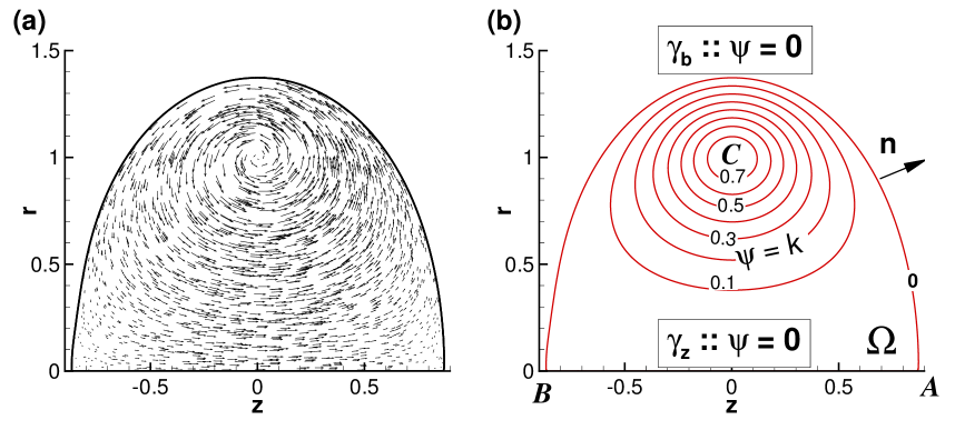
Figure 1: Direct numerical simulation of the incompressible Navier-Stokes equations representing a physical vortex ring with axial symmetry [14]. Velocity vectors (a) and corresponding streamlines (b) in the frame of reference travelling with the vortex ring.

Classical vortex ring models are stationary solutions of Euler equations. The key feature of such models is that the vorticity transport equation reduces to (e. g. [15, 16])

$$\frac{\omega}{r}=\left\{\begin{tabular}[]{ll}$f(\psi)$&\mbox{in} \,\, $\Omega_{b}$,\\ 0&\mbox{elsewhere},\end{tabular}\right.$$ (1)

with $f:{\mathbb{R}}\rightarrow{\mathbb{R}}$ called the vorticity function (it is related to the source function introduced above as $F(\psi)=rf(\psi)$). In other words, $\omega$ propagates with a time-invariant profile $f(\psi)$ along streamlines in the frame of reference moving with the vortex. As described in detail in the next section, the associated mathematical problem consists in solving an elliptic PDE for $\psi$ with a right-hand-side term depending on the solution itself. The main difficulty in solving this PDE comes from the fact that the boundary $\partial\Omega_{b}$ of the vortex bubble is not known in advance, which makes it a free boundary problem.

The only known analytical solution of this problem considers $f(\psi)=const$ within $\Omega_{b}$ which has the shape of a sphere, and is known as Hill’s spherical vortex [17] (see also [15, 16]). The mathematical theory of inviscid axisymmetric vortex rings was developed in the ’70s and in the early ’80s [18] around Hill’s vortex, by considering the following particular form of the vorticity function

$$f(\psi)=const,\quad\forall\psi>k,\qquad\mbox{and}\qquad f(\psi)=0,\quad\forall\psi\leq k,$$ (2)

with $k>0$ defining the vortex-ring core as $\Omega_{c}=\left\{({z,r,\theta})\in{\mathbb{R}}^{3},\psi(z,r)>k\right\}\subset\Omega_{b}$ (see Figure 1b). Existence and uniqueness results for the inviscid vortex ring problem are presented in [18, 19, 20] for the general case and in [21, 22] for vortex rings bifurcating from Hill’s vortex. Numerical solutions of the vortex-ring problem, using (2) as the vorticity function, were obtained by Norbury [23] and Fraenkel [24], and are hereafter referred to as NF vortices. These models were also extended to allow for vortex rings with swirl (i.e., with nonzero azimuthal velocity); analytical closed-form solutions for Hill’s spherical vortex with swirl were obtained in [25] and numerical solutions using vorticity functions generalizing (2) for swirling flows were presented in [26].

From the practical point of view, vortex-ring models are useful as inviscid approximations to actual vortex structures observed in experiments or generated by the Direct Numerical Simulation (DNS) of the Navier-Stokes equations. For the purposes of fitting such models to DNS data, the NF inviscid vortex-ring model [24, 23] was widely adopted and proved very useful in estimating integral quantities and global properties of actual vortex rings [27, 28, 29]. This is quite remarkable, since the vorticity function (2) gives a linear vorticity distribution in the vortex core, i. e. proportional to the distance from the axis of symmetry, which is in fact quite different from the Gaussian vorticity distribution typically observed in experiments (e. g. [30, 31]). The main feature of the inviscid vortex-ring models is that the vorticity function $f(\psi)$ is prescribed by (1) as a hypothesis of the model. While experimental studies [32, 33] reported some scatter in the plots of $\omega/r$ versus $\psi$, this data was rather well fitted by an empirical formula for the vorticity function in the exponential form $f(\psi)=a\exp(b\psi)$ with $a$ and $b$ representing two constants adjusted during the fitting procedure [33]. This supports the idea that steady inviscid models could be used as good approximations of unsteady viscous vortex rings arising in real flows if the vorticity function $f(\psi)$ is accurately determined.

In the present contribution we formulate the problem of identifying an optimal vorticity function $f(\psi)$ as an inverse problem. It will be solved using a variational optimization approach in which optimality of the reconstruction implies that the obtained inviscid vortex-ring model best matches, in a suitably defined sense, the available measurements. A natural question in the formulation of such an inverse problem is how much measurement data is required to ensure a reliable reconstruction The solution method we have developed can assimilate measurements available in 3D regions or on 2D surfaces with in principle arbitrary shapes. While modern experimental techniques such as particle-image velocimetry (PIV) and advanced DNS can provide snapshots of the velocity field in a large part of the flow domain, for benchmarking purposes in our computational examples we will consider an arguably harder problem where only incomplete measurements are available. More specifically, we will assume the reconstructions to be based on measurements of the tangential velocity component on $\partial\Omega_{b}$, the boundary of the vortex bubble. A practical application in which this situation occurs is the experimental study of fuel injection in automobile engines [3, 4, 8]: measurements in the injected two-phase spray do not always provide reliable velocity fields in the vortex bubble $\Omega_{b}$ because of the high density of seeding particles [34]. It is then necessary to theoretically reconstruct parts of the flow field not accessible to measurements. As demonstrated by the results of our test problem concerning Hill’s vortex, even in such a restricted setting, the vorticity function can be accurately reconstructed with our approach. In our second example based on actual DNS data, we will show how the proposed approach can improve the accuracy of an inviscid vortex model derived from a purely empirical fit for the vorticity function. The predictions of our model will also be compared to classical reconstruction methods based on fitting theoretical vortex-ring models to the entire velocity field inside the vortex-ring bubble. We will show that our approach offers a good approximation of both the structure of the vorticity field and its integral characteristics, which is not the case with classical reconstruction methods. This is quite remarkable, since only partial information about the velocity field is used in our method.

The structure of the paper is as follows: in the next two sections we introduce the equations satisfied by the steady inviscid vortex rings and formulate the reconstruction problem in terms of an optimization approach. In Section 4 we propose a gradient-based solution method and derive the gradient formula. The computational algorithm is described in Section 5, together with the tests validating the method used for the computation of the gradients. The proposed method is first validated against a known analytical solution (Hill’s vortex) in Section 6. The approach is then applied to a challenging problem of reconstructing an optimal vorticity function from realistic DNS data in Section 7. Discussion and final conclusion are deferred to Section 8.

2 Physical Problem and Governing Equations

In this section we present the equations satisfied by our vortex model. We consider incompressible axisymmetric vortex rings without swirl and add that formally a very similar description also holds for 2D inviscid flows. If a stationary solution is sought, it is more convenient to describe the flow in the frame of reference moving with the translation velocity $W{\bf e}_{z}$ (assumed constant) of the vortex ring (see Figure 1). A divergence-free velocity field is constructed by defining the Stokes streamfunction $\psi$ [15, 16] such that

$$v_{z}=\frac{1}{r}\frac{\partial\psi}{\partial r},\quad v_{r}=-\frac{1}{r}\frac{\partial\psi}{\partial z},\quad v_{\theta}=0.$$ (3)

The azimuthal component of the vorticity vector is then given by

$$\omega=\frac{\partial v_{r}}{\partial z}-\frac{\partial v_{z}}{\partial r}.$$ (4)

Combining (3) and (4) results in an elliptic partial differential equation for the streamfunction

$${\mathcal{L}}\psi=-\omega\quad\mbox{in}\,\,\Pi=\left\{(z,r)\in{\mathbb{R}}^{2},r>0\right\},$$ (5)

where ${\mathcal{L}}$ is defined as

$$\quad{\mathcal{L}}:=\frac{\partial}{\partial z}\left(\frac{1}{r}\frac{\partial}{\partial z}\right)+\frac{\partial}{\partial r}\left(\frac{1}{r}\frac{\partial}{\partial r}\right)=\boldsymbol{\nabla}\cdot\left(\frac{1}{r}\boldsymbol{\nabla}\right),\quad\text{where}\ \boldsymbol{\nabla}:=\left({\frac{\partial}{\partial z}},{\frac{\partial}{\partial r}}\right)^{T}.$$ (6)

The boundary condition required for equation (5) accounts for an external flow around the vortex which is uniform at infinity with velocity $-W{\bf e}_{z}$ (see Figure 1)

$$\Psi:=\psi+\frac{1}{2}Wr^{2}\rightarrow 0\quad\mbox{as}\quad|{\bf x}|:=\sqrt{z^{2}+r^{2}}\rightarrow\infty.$$ (7)

We note that $\Psi$ is the Stokes streamfunction in the laboratory frame of reference; $\Psi$ also satisfies the PDE (5), since ${\mathcal{L}}(k+\frac{1}{2}Wr^{2})=0$ for any constants $W$ and $k$.

We recall that for inviscid and steady flows in the frame of reference moving with the vortex ring, the transport equation for the vorticity reduces to (1). Problem (5) can be reduced to a semi-linear elliptic system by considering a particular form of the vorticity function as given, for example, in (2) [18]. A different reformulation of the problem, namely, as a semi-linear Dirichlet boundary-value problem for the Laplacian operator in cylindrical coordinates in ${\mathbb{R}}^{5}$, was introduced in [19]. This made possible the use of variational techniques to prove existence results [19, 35], symmetry [36] and asymptotic behaviour [37] of solutions.

In the present study, we formulate the vortex-ring problem in the domain $\Omega\subset{\mathbb{R}}^{2}$ defined as the cross-section of the vortex bubble $\Omega_{b}$ in the meridian half plane $r>0$ (see Figure 1b). The domain $\Omega$ is then bounded by the dividing streamline ($\psi=0$) containing the front ($A$) and rear ($B$) stagnation points. On the axis of symmetry ($r=0$) the radial velocity $v_{r}$ vanishes which is consistent with the relation $\psi=0$ holding there. These two parts of the boundary of the vortex bubble will be denoted $\gamma_{b}$ and $\gamma_{z}$, respectively. Thus, the governing system for vortex rings takes the final form

$${\mathcal{L}}\psi =-r\,f(\psi) \textrm{in}\ \Omega,$$ (8a)

$$\psi =0 \textrm{on}\ \gamma:=\gamma_{z}\cup\gamma_{b}.$$ (8b)

Although the fore-and-aft symmetry is not enforced in solving system (8), most (albeit not all) solutions of this system obtained in our study will have this property. Hereafter we will use as diagnostic quantities the following integral characteristics of the vortex rings: circulation $\Gamma$, impulse (in the horizontal direction $z$) $I$, and energy $E$. Using the vorticity function $f(\psi)$, they can be expressed [16] in terms of the following integrals over domain $\Omega$ (figure 1b)

$$\Gamma :=\int_{\Omega}rf(\psi(z,r))\,drdz,$$ (9a)

$$I :=\pi\int_{\Omega}r^{3}f(\psi(z,r))\,drdz,$$ (9b)

$$E :=\pi\int_{\Omega}rf(\psi(z,r))\psi(z,r)\,drdz.$$ (9c)

3 Formulation of the Reconstruction Problem

In this section we formulate the reconstruction problem as an inverse problem of source identification amenable to solution using variational optimization techniques. Before we can precisely state this formulation, we need to characterize the admissible vorticity functions $f$. Their domain of definition will be restricted to the interval ${\mathcal{I}}:=[0,\psi_{\max}]$, where $\psi_{\max}>\max_{{\bf x}\in\Omega}\psi({\bf x})$ is chosen arbitrarily, so that $f\;:\;{\mathcal{I}}\rightarrow{\mathbb{R}}$. We will refer to ${\mathcal{I}}$ as the “identifiability interval” [9]. Next, we note that in order to guarantee the existence of nontrivial solutions to nonlinear elliptic boundary-value problems of the type (8), the vorticity function $f(\psi)$ must be positive (we refer the reader to the monographs [38, 39] for a more detailed discussion of this issue). Regarding the regularity of the vorticity function, we will restrict our attention to continuous functions $f$ which is required due to certain technical aspects of the reconstruction algorithm (see Section 44.2). While this assumption does exclude vortex-ring models with vorticity support compact in $\Omega_{b}$, such as the NF model, cf. relation (2), such continuous vorticity functions are more appropriate for practical applications motivating this study. More specifically, we will assume that $f$ belongs to the Sobolev space $H^{1}({\mathcal{I}})$ of continuous functions defined on ${\mathcal{I}}$ with square-integrable gradients. The inner product defined in this space is

$$\forall_{z_{1},z_{2}\in H^{1}({\mathcal{I}})}\qquad\big{\langle}z_{1},z_{2}\big{\rangle}_{{H^{1}({\mathcal{I}})}}=\int_{0}^{\psi_{\text{max}}}z_{1}z_{2}+{\ell^{2}}{\frac{\partial z_{1}}{\partial s}}{\frac{\partial z_{2}}{\partial s}}\,ds,$$ (10)

where $\ell\in{\mathbb{R}}^{+}$ is a parameter with the meaning of a “length scale” (the significance of this parameter will be discussed further in Section 44.3). We can now state the reconstruction problem as follows

Problem 1

Given the measurements $m\;:\;\gamma_{b}\cup\gamma_{z}\rightarrow{\mathbb{R}}$ of the velocity component tangential to the boundaries $\gamma_{b}$ and $\gamma_{z}$, find a vorticity function $\hat{f}\in H^{1}({\mathcal{I}})$, such that the corresponding solution of (8) matches data $m$ as well as possible in the least-squares sense.

For the purpose of the numerical solution, we will recast Problem 1 as a variational optimization problem which can be solved using a suitable gradient-based method. Since the tangential velocity at the boundary is ${{\bf v}}\cdot{\bf n}^{\perp}=\frac{1}{r}{\frac{\partial\psi}{\partial n}}$, we define a cost functional ${\mathcal{J}}\;:\;H^{1}({\mathcal{I}})\rightarrow{\mathbb{R}}$ as

$${\mathcal{J}}(f):=\frac{\alpha_{b}}{2}\int_{\gamma_{b}}\left(\frac{1}{r}{\frac{\partial\psi}{\partial n}}\bigg{|}_{\gamma_{b}}-m\right)^{2}\,d\sigma+\frac{\alpha_{z}}{2}\int_{\gamma_{z}}\left(\frac{1}{r}{\frac{\partial\psi}{\partial n}}\bigg{|}_{\gamma_{z}}-m\right)^{2}\,d\sigma,$$ (11)

where $\alpha_{b}$ and $\alpha_{z}$ assume the values $\{0,1\}$ depending on which part(s) of the domain boundary the measurements are available on. At this point we remark that measurement data distributed over some finite-area region ${\mathcal{R}}\in\Omega$ can also be used and in such case the line integrals in (11) will be replaced with suitable area integrals over ${\mathcal{R}}$. The optimal reconstruction $\hat{f}$ will thus be obtained via solution of the following minimization problem

$$\hat{f}:=\operatorname{argmin}_{f\in H^{1}({\mathcal{I}})}\ {\mathcal{J}}(f),$$ (12)

where “$\operatorname{argmin}$” denotes the argument minimizing the objective function. In some situations it may be necessary to enforce the nonnegativity $f(\psi)\geq 0$ of the vorticity function (functions obtained by imposing this property will be denoted $f_{+}$). Rather than including an inequality constraint in optimization problem (12), this can be achieved in a straightforward manner by expressing $f_{+}=(1/2)g^{2}$, where $g$ is a real-valued function defined on ${\mathcal{I}}$, and then recasting problem (12) in terms of the new function $g$ as the control variable.

Problem 1 is an example of an inverse problem of source identification. However, in contrast to the most common problems of this type [13], in which the source function depends on the independent variables (e.g., on ${\bf x}$), in Problem 1 the source $f$ is sought as a function of the state variable $\psi$. As will be shown in the following section, to address this aspect of the problem, a specialized version of the adjoint-based gradient approach will be developed.

4 Gradient-Based Solution Approach

In this section we first describe the general optimization formulation which is followed by the derivation of a convenient expression for the cost functional gradient. Finally, we discuss the calculation of smoothed Sobolev gradients.

4.1 Minimization Algorithm

For simplicity, the solution approach to Problem 1 we present below will not address the positivity constraint which can be accounted for in a straightforward manner using the substitution mentioned at the end of the previous section. Solutions to problem (12) are characterized by the following first-order optimality condition

$$\forall_{f^{\prime}\in H^{1}({\mathcal{I}})}\quad{\mathcal{J}}^{\prime}(\hat{f};f^{\prime})=0,$$ (13)

where the Gâteaux differential ${\mathcal{J}}^{\prime}(f;f^{\prime}):=\lim_{\epsilon\rightarrow 0}\epsilon^{-1}\left[{\mathcal{J}}(f+\epsilon f^{\prime})-{\mathcal{J}}(f)\right]$ of functional (11) is

$${\mathcal{J}}^{\prime}(f;f^{\prime})=\alpha_{b}\int_{\gamma_{b}}\left(\frac{1}{r}{\frac{\partial\psi}{\partial n}}\bigg{|}_{\gamma_{b}}-m\right)\,\frac{1}{r}{\frac{\partial\psi^{\prime}}{\partial n}}\bigg{|}_{\gamma_{b}}d\sigma+\alpha_{z}\int_{\gamma_{z}}\left(\frac{1}{r}{\frac{\partial\psi}{\partial n}}\bigg{|}_{\gamma_{z}}-m\right)\,\frac{1}{r}{\frac{\partial\psi^{\prime}}{\partial n}}\bigg{|}_{\gamma_{z}}d\sigma,$$ (14)

in which the variable $\psi^{\prime}$ satisfies the linear perturbation equation

$$\boldsymbol{\nabla}\cdot\left(\frac{1}{r}\boldsymbol{\nabla}\psi^{\prime}\right)+rf_{\psi}(\psi)\,\psi^{\prime} =-r\,f^{\prime} \textrm{in}\ \Omega,$$ (15a)

$$\psi^{\prime} =0 \textrm{on}\ \gamma,$$ (15b)

where $f_{\psi}:=\dfrac{df}{d\psi}$ and $f^{\prime}$ is the “direction” in which the differential is computed in (14). The presence of the derivative $f_{\psi}$ in (15a) is the reason explaining the regularity requirements imposed on $f$ (cf. Section 4).

The optimal reconstruction can be obtained as $\hat{f}=\lim_{k\rightarrow\infty}f^{(k)}$, where the approximations $f^{(k)}$ can be computed with the following gradient descent algorithm

$$f^{(k+1)} =f^{(k)}-\tau_{k}\nabla{\mathcal{J}}(f^{(k)}),\quad k=1,2,\dots$$ (16)

$$f^{(1)} =f_{0},$$

in which $f_{0}$ is the initial guess and $\tau_{k}$ represents the length of the step along the descent direction at the $k$-th iteration. For the sake of simplicity, formulation (16) corresponds to the steepest-descent algorithm, however, in actual computations we shall prefer more advanced minimization techniques, such as the conjugate gradient method [40] (see Section 5). We note that optimality condition (13) and the associated gradient descent (16) characterize only local minimizers and establishing a priori whether a given minimizer is global is not possible. This is a consequence of the nonconvexity of Problem 1 resulting from the nonlinearity of governing system (8). Global maximizers are sought by solving problem (16) repeatedly using a range of different initial guesses $f_{0}$.

4.2 Derivation of the Gradient Expression

A key element of descent algorithm (16) is the cost functional gradient $\nabla{\mathcal{J}}(f)$. Assuming that Gâteaux differential (14) is a bounded linear functional defined on a Hilbert space ${\mathcal{X}}$ (e.g., ${\mathcal{X}}=L_{2}({\mathcal{I}})$ or ${\mathcal{X}}=H^{1}({\mathcal{I}})$), i.e., ${\mathcal{J}}^{\prime}(f;\cdot)\;:\;{\mathcal{X}}\rightarrow{\mathbb{R}}$, an expression for the gradient $\nabla^{{\mathcal{X}}}{\mathcal{J}}(f)$ can be obtained from (14) employing the Riesz representation theorem [41]

$${\mathcal{J}}^{\prime}(f;f^{\prime})=\Big{\langle}\nabla^{{\mathcal{X}}}{\mathcal{J}}(f),f^{\prime}\Big{\rangle}_{{\mathcal{X}}},$$ (17)

with $\langle.,.\rangle_{{\mathcal{X}}}$ denoting the inner product in the space ${\mathcal{X}}$. We note that representation (14) is not yet consistent with (17), since the perturbation $f^{\prime}$ is not explicitly present in it, but is instead hidden in the source term of perturbation equation (15a). In order to identify an expression for the gradient consistent with (17), we introduce the adjoint variable $\psi^{*}\;:\;\Omega\rightarrow{\mathbb{R}}$. Integrating (15a) against $\psi^{*}$ over $\Omega$ and then integrating by parts twice we obtain

$$0= \int_{\Omega}\psi^{*}\,\left[\boldsymbol{\nabla}\cdot\left(\frac{1}{r}\boldsymbol{\nabla}\psi^{\prime}\right)+rf_{\psi}(\psi)\,\psi^{\prime}\right]\,d\Omega+\int_{\Omega}\psi^{*}\,r\,f^{\prime}d\Omega$$ (18)

$$= \int_{\Omega}\psi^{\prime}\,\left[\boldsymbol{\nabla}\cdot\left(\frac{1}{r}\boldsymbol{\nabla}\psi^{*}\right)+rf_{\psi}(\psi)\,\psi^{*}\right]\,d\Omega+\int_{\Omega}\psi^{*}\,r\,f^{\prime}d\Omega$$

$$+\int_{\gamma_{b}\cup\gamma_{z}}\frac{1}{r}\left(\psi^{*}{\frac{\partial\psi^{\prime}}{\partial n}}-\psi^{\prime}{\frac{\partial\psi^{*}}{\partial n}}\right)\,d\sigma.$$

Using boundary condition (15b) and defining the adjoint system as follows

$$\boldsymbol{\nabla}\cdot\left(\frac{1}{r}\boldsymbol{\nabla}\psi^{*}\right)+rf_{\psi}(\psi)\,\psi^{*} =0 \textrm{in}\ \Omega,$$ (19a)

$$\psi^{*} =\alpha_{b}\left(\frac{1}{r}{\frac{\partial\psi}{\partial n}}\bigg{|}_{\gamma_{b}}-m\right) \textrm{on}\ \gamma_{b},$$ (19b)

$$\psi^{*} =\alpha_{z}\left(\frac{1}{r}{\frac{\partial\psi}{\partial n}}\bigg{|}_{\gamma_{z}}-m\right) \textrm{on}\ \gamma_{z},$$ (19c)

identity (18) simplifies to

$${\mathcal{J}}^{\prime}(f;f^{\prime})=-\int_{\Omega}\psi^{*}\,r\,f^{\prime}d\Omega.$$ (20)

Although perturbation $f^{\prime}$ appears explicitly in (20), this expression still is not in a form consistent with Riesz representation (17), because the latter requires an inner product with $s$ (equivalently, $\psi$) as the integration variable. We address this issue by expressing $f^{\prime}(\psi)$ in terms of the following integral transform

$$f^{\prime}(\psi({\bf x}))=\int_{0}^{\psi_{\max}}\delta(\psi({\bf x})-s)f^{\prime}(s)\,ds,\quad{\bf x}\in\Omega,$$ (21)

where $\delta(\cdot)$ is the Dirac delta distribution. Plugging (21) into (20) and then using Fubini’s theorem to exchange the order of integration, we obtain

$${\mathcal{J}}^{\prime}(f;f^{\prime}) =-\int_{\Omega}\psi^{*}\,r\,\left[\int_{0}^{\psi_{\max}}\delta(\psi({\bf x})-s)f^{\prime}(s)\,ds\right]d\Omega$$ (22)

$$=-\int_{0}^{\psi_{\max}}f^{\prime}(s)\left[\int_{\Omega}\psi^{*}\,r\,\delta(\psi({\bf x})-s)\,d\Omega\right]\,ds$$

which is already consistent with Riesz representation (17). Although this is not the gradient used in our actual calculations, we first identify the $L_{2}$ gradient of ${\mathcal{J}}$ and then obtain from it the required Sobolev gradient $\nabla^{H^{1}}{\mathcal{J}}$ as shown in Section 44.3. Thus, setting ${\mathcal{X}}=L_{2}({\mathcal{I}})$, relation (17) becomes ${\mathcal{J}}^{\prime}(f;f^{\prime})=\int_{{\mathcal{I}}}\nabla{\mathcal{J}}(s)f^{\prime}(s)\,ds$ which, together with (22), yields

$$\nabla^{L_{2}}{\mathcal{J}}(s)=-\int_{\Omega}\psi^{*}\,r\,\delta(\psi({\bf x})-s)\,d\Omega=-\int_{\gamma_{s}}\psi^{*}\,r\,\left({\frac{\partial\psi}{\partial n}}\right)^{-1}\,d\sigma,\quad s\in[0,\psi_{\max}].$$ (23)

The expression on the right-hand side (RHS) of (23) shows that, for a given $s\in{\mathcal{I}}$, the gradient $\nabla^{L_{2}}{\mathcal{J}}(s)$ can be evaluated as a contour integral on the level set

$$\gamma_{s}:=\{{\bf x}\in\Omega\,:\,\psi({\bf x})=s\}.$$ (24)

We add that an essentially identical approach will remain applicable when the measurements are available over a finite-area region ${\mathcal{R}}$ rather than on the contours $\gamma_{b}$ and $\gamma_{z}$. The only difference is that the adjoint system will be “forced” through a source term (with the support equal to ${\mathcal{R}}$) on the RHS of (19a), instead of through boundary conditions (19b)–(19c) as discussed above.

4.3 Sobolev Gradients

We now proceed to discuss how Sobolev gradients $\nabla{\mathcal{J}}=\nabla^{H^{1}}{\mathcal{J}}$ employed in gradient-descent approach (16) can be derived from the $L_{2}$ gradients obtained in (23). We remark that this additional regularity is required for the consistency of the entire approach, since the reconstruction with $L_{2}$ gradients would not guarantee (weak) differentiability of the vorticity function $f(\psi)$, thus rendering adjoint system (19) ill-posed (because of the term $f_{\psi}$ in (19a)). This will be done using inner product (10) in Riesz identity (17). In addition to enforcing smoothness of the reconstructed vorticity functions, this formulation also allows us to impose the desired behavior at the endpoints of interval ${\mathcal{I}}$ via suitable boundary conditions (we refer the reader to [9] for a more in-depth discussion of these issues). As regards the behavior of the gradients $\nabla^{H^{1}}{\mathcal{J}}$ at the endpoints of interval ${\mathcal{I}}$, we can require the vanishing of either the gradient itself or its derivative with respect to $s$. In the present study we prescribe the homogeneous Neumann boundary condition at the right endpoint of the identifiability interval ${\mathcal{I}}$

$$\frac{d}{ds}(\nabla^{H^{1}}{\mathcal{J}})=0\quad\textrm{at}\ s=\psi_{\text{max}}$$ (25)

which implies that, with respect to the initial guess $f_{0}$, at $s=\psi_{\text{max}}$ iterations (16) can modify the values, but not the slope, of the reconstructed functions $f^{(k)}$. As regards the behavior of the Sobolev gradients at the left endpoint, we will consider either Dirichlet or Neumann boundary conditions

$$\nabla^{H^{1}}{\mathcal{J}} =0\quad \textrm{at}\ s=0,$$ (26a)

$$\frac{d}{ds}(\nabla^{H^{1}}{\mathcal{J}}) =0\ \textrm{at}\ s=0$$ (26b)

which will preserve, respectively, the value or the slope of the initial guess $f_{0}$ at $s=0$. We refer the reader to [11] for a discussion of other possible choices of boundary conditions imposed on the Sobolev gradients in an identification problem with a similar structure. We emphasize that the choice of the boundary behavior of the Sobolev gradients plays in fact a significant role from the physical point of view. Together with the behaviour of the initial guess $f_{0}$ in the neighbourhood of $s=0$ and $s=\psi_{\text{max}}$, it expresses our hypotheses on the properties of the optimal reconstruction $\hat{f}(\psi)$ for the limiting values of $\psi$ where no measurement data is available. The need to supplement measurement data with some auxiliary information about the solution is quite typical for inverse problems [42]. Additional comments about the specific physical meaning of the boundary conditions imposed on the Sobolev gradients will be provided in Sections 6 and 7.

Identifying expression (17) in which ${\mathcal{X}}=H^{1}({\mathcal{I}})$ with the inner product given in (10), integrating by parts and using boundary conditions (25)–(26) we obtain the following elliptic boundary-value problem on ${\mathcal{I}}$ defining the Sobolev gradient $\nabla^{H^{1}}{\mathcal{J}}$

$${\left(I-{\ell}^{2}\frac{d^{2}}{ds^{2}}\right)}\nabla^{H^{1}}{\mathcal{J}} =\nabla^{L_{2}}{\mathcal{J}} \textrm{in}\ {\mathcal{I}},$$ (27a)

$$\left.\begin{aligned} \nabla^{H^{1}}{\mathcal{J}}\quad&\\ \frac{d}{ds}\nabla^{H^{1}}{\mathcal{J}}\quad&\end{aligned}\right\} =0 \textrm{at}\ s=0,$$ (27b)

$$\frac{d}{ds}\nabla^{H^{1}}{\mathcal{J}} =0 \textrm{at}\ s=\psi_{\text{max}},$$ (27c)

where the expression for $\nabla^{L_{2}}{\mathcal{J}}$ is given in (23). A slightly different way of obtaining Sobolev gradients in identification problems with analogous structure is discussed in [9].

It is well known [43] that extraction of cost functional gradients in the space $H^{1}$ with the inner product defined as in (10) can be regarded as low-pass filtering of $L_{2}$ gradients with the cut-off wavenumber given by $\ell^{-1}$. The quantity $\ell$ admits a clear physical meaning as the smallest “length-scale” (with the magnitude of the streamfunction $\psi$ playing the role of “length”) which is retained when the Sobolev gradient is extracted according to (27). In other words, features of the $L_{2}$ sensitivity (23) with characteristic length scales smaller than $\ell$ are removed during gradient preconditioning. Therefore, by choosing $\ell$ to represent the characteristic variation of the streamfunction $\psi$ in the problem, this mechanism allows us to eliminate in a controlled manner undesired small-scale components which may be present in the $L_{2}$ gradients due to noise in the measurements, numerical approximation errors, etc. One approach which has been found to work particularly well [43] is to start with a relatively large value of $\ell$, which gives smooth gradients suitable for reconstructing large-scale features of the solution, and then decrease it with iterations, which allows one to zoom in on progressively smaller features of the solution. This is the approach we adopt here by setting $\ell^{(k)}$, the value of the length-scale used in (27) at the $k$-th iteration, as

$$\ell^{(k)}=\zeta^{k}\,\ell^{(0)},\quad k>0,$$ (28)

where $\ell^{(0)}$ is some initial value and $0<\zeta<1$ the decrement factor.

5 Computational Algorithm

As is evident from Section 3, the reconstruction algorithm requires the solution of several linear and nonlinear elliptic boundary-value problems in one or two spatial dimensions, namely, the governing system (8), the adjoint system (19) and the preconditioning system for the Sobolev gradients (27). In addition, evaluation for the $L_{2}$ gradients is somewhat involved, because the integrals in (23) are evaluated on the level sets $\gamma_{s}$ which have to be identified, cf. definition (24). All of these technical issues were easily handled using the freely available finite-element software FreeFem++ [44, 45]. This generic PDE solver offers the possibility of using a large variety of triangular finite elements with an integrated grid generator in two or three dimensions. FreeFem++ is equipped with its own high-level programming language with syntax close to mathematical formulations. It was recently used to solve different types of partial differential equations, e. g. Schrödinger and Gross-Pitaevskii equations [46, 47], incompressible Navier-Stokes equations [10], Poisson equations with nonlinear source terms [48] and Navier-Stokes-Boussinesq equations [49]. The main advantage of employing FreeFem++ for the present problem is the simplicity in using different finite-element meshes for each sub-problem making the interpolation or computation of integrals very easy and accurate. Below we briefly describe the implementation of key elements of the computational algorithm which are then validated in the following section.

5.1 Main Computational Modules

The computational algorithm consists of the following main modules:

$\bullet$ [Definition of the mesh and the associated finite-element spaces] We define here the boundaries $\gamma_{b}$ and $\gamma_{z}$ and build a triangular mesh covering the vortex domain $\Omega$ (see Figure 2). The mesh density is characterized by $N_{x}$ representing the number of segments per unit length in the discretization of the domain boundaries. The finite element space $V_{h}$ is defined such that all dependent variables are represented using piecewise quadratic $P^{2}$ finite elements. Cost function (11) is computed with a 6-th order Gauss quadrature formula.

$\bullet$ [One-dimensional interpolation] The vorticity function $f(s)$ is tabulated at $N_{f}$ discrete values $s_{i}\in[0,\psi_{\max}]$, $i=1,\dots,N_{f}$. The value $\psi_{\max}$ (cf. Section 3) is set depending on a particular reconstruction case. To obtain values of $f$ and its derivative $f_{\psi}$ for non-tabulated values of $\psi$ we use cubic spline interpolation.

$\bullet$ [Solution of direct problem (8)] Given the nonlinearity of this problem, we use Newton’s method with $p$-th iteration consisting in computing the solution $q:=(\psi^{p}-\psi^{p+1})$ of the following variational problem

$$\int_{\Omega}\frac{1}{r}\boldsymbol{\nabla}q\cdot\boldsymbol{\nabla}v\,d\Omega-\int_{\Omega}{rf_{\psi}(\psi^{p})}qv\,d\Omega=\int_{\Omega}\frac{1}{r}\boldsymbol{\nabla}\psi^{p}\cdot\boldsymbol{\nabla}v\,d\Omega-\int_{\Omega}{rf(\psi^{p})}v\,d\Omega,\quad\forall v\in V_{h}.$$ (29)

This problem is solved efficiently in FreeFem++ by building the corresponding matrices (spline interpolation is used to evaluate $f(\psi({\bf x}))$ and $f_{\psi}(\psi({\bf x}))$). Newton’s iterations are stopped when $\|q\|_{2}\leq\varepsilon_{N}$ with $\varepsilon_{N}=10^{-6}$.

$\bullet$ [Solution of adjoint problem (19)] Given the linearity of this problem, this consists in solving the weak formulation

$$\int_{\Omega}-\frac{1}{r}\boldsymbol{\nabla}\psi^{*}\boldsymbol{\nabla}v\,d\Omega+\int_{\Omega}{rf_{\psi}(\psi)}\psi^{*}v\,d\Omega=0,\quad\forall v\in V_{h},$$ (30)

with Dirichlet boundary conditions (19b)-(19c), which takes two lines of code in FreeFem++.

$\bullet$ [Computation of $L_{2}$ gradient] To use formula (23) for the $L_{2}$ gradient $\nabla^{L_{2}}{\mathcal{J}}(s)$, for each value $s_{i}$, $i=1,\dots,N_{f}$, in the table defining the discretized vorticity function $f(s_{i})$, we construct the corresponding level set $\gamma_{s_{i}}$ and mesh its interior (see Figure 2). The values of $\psi^{*}$ and $\psi$ are $P^{2}$ interpolated on the new mesh and the integral in (23) is then computed with a 6-th order Gauss quadrature formula.

$\bullet$ [Computation of $H^{1}$ gradient] To obtain the $H^{1}$ gradient from the $L_{2}$ gradient we solve the one-dimensional boundary-value problem (27) with either (27b) or (27c) as the boundary condition. This is a standard problem which can be solved in a straightforward manner using $P^{1}$ piecewise linear finite elements or second-order accurate centered finite differences.

$\bullet$ [Minimization algorithm] With the cost functional gradient evaluated as described above, we approximate the optimal vorticity function $\hat{f}$ using the Polak-Ribiere variant of the conjugate gradients algorithm [40] which is an improved version of descent algorithm (16). The length of the step $\tau_{k}$ at every iteration $k$ is determined by solving a line minimization problem

$$\tau_{k}=\underset{\tau>0}{\operatorname{argmin}}\;{\mathcal{J}}(f^{(k)}-\tau\,\boldsymbol{\nabla}{\mathcal{J}}(f^{(k)}))$$ (31)

using Brent’s method [50].

Clearly, accurate evaluation of the cost functional gradients $\boldsymbol{\nabla}{\mathcal{J}}(f)$ is a key element of the proposed reconstruction approach and these calculations are thoroughly validated in the following section.

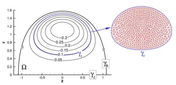
Figure 2: Schematic of the calculation of the $L_{2}$ gradient of the cost functional based on formula (23). The level set $\gamma_{s}$ corresponding to $s=0.1$ is marked with a thick line, whereas the inset represents the mesh discretizing the domain bounded by $\gamma_{s}$.

5.2 Validation of Cost Functional Gradients

In this section we analyze the consistency of the gradient $\boldsymbol{\nabla}{\mathcal{J}}$ evaluated based on formula (23) with respect to refinement of the two key numerical parameters in the problem, namely, $N_{x}$ and $N_{f}$ (see the previous section for definitions). A standard test [51] consists in computing the Gâteaux differential ${\mathcal{J}}^{\prime}(f;f^{\prime})$ in some arbitrary direction $f^{\prime}$ using relations (22)–(23) and comparing it to the result obtained with a forward finite–difference formula. Thus, deviation of the quantity

$$\kappa(\epsilon):=\frac{\epsilon^{-1}\left[{\mathcal{J}}(\psi_{b}+\epsilon\psi^{\prime}_{b})-{\mathcal{J}}(\psi_{b})\right]}{\int_{0}^{\psi_{\max}}f^{\prime}(s)\boldsymbol{\nabla}{\mathcal{J}}(s)\,ds}$$ (32)

from the unity is a measure of the error in computing ${\mathcal{J}}^{\prime}(f;f^{\prime})$ (we note that, in the light of identity (17), expression in the denominator of (32) may be based on the $L_{2}$ gradients).

The dependence of the quantity $\log|\kappa(\epsilon)-1|$, which captures the number of significant digits of accuracy achieved in the evaluation of (32), on $\epsilon$ is shown in Figures 3a and 3b, respectively, for increasing $N_{f}$ and $N_{x}$ while keeping the other parameter fixed.

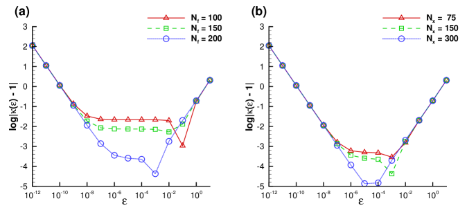
Figure 3: Dependence of the diagnostic quantity $\kappa(\epsilon)$ defined in (32) on $\epsilon$ for (a) different discretizations of the identifiability interval ${\mathcal{I}}$ given by $N_{f}=100,150,200$ with $N_{x}=150$ fixed, and (b) different discretizations of the domain $\Omega$ given by $N_{x}=75,150,300$ with $N_{f}=200$ fixed.

These results were obtained in a configuration representing Hill’s vortex in which $C=1/2$ and $\Omega$ is a half-circle of radius $a=2$ (see Section 6 for a precise definition of this test problem), and some generic forms of the reference vorticity function $f$ and its perturbation $f^{\prime}$ were used. As is evident from Figures 3a and 3b, the values of $\kappa(\epsilon)$ approach the unity for $\epsilon$ ranging over approximately 7 orders of magnitude as the discretization is refined (i.e., as $N_{f}$ and $N_{x}$ increase). We emphasize that, since we are using the “differentiate–then–discretize” rather than “discretize–then–differentiate” approach, the gradient should not be expected to be accurate up to the machine precision [52]. This is because of the presence of small, but nonzero, errors in the approximation of the different PDEs and the gradient expression (23). The deviation of $\kappa(\epsilon)$ from the unity for very small values of $\epsilon$ is due to the arithmetic round–off errors, whereas for the large values of $\epsilon$ it is due to the truncation errors, both of which are well known effects [51]. In particular, the former effect is typical of all finite-difference techniques and as such is an artifact of formula (32) usually employed to test the accuracy of adjoint-based gradient expressions. These results thus demonstrate high accuracy of the computed gradients and confirm that this accuracy can be systematically improved by refining the discretization.

The computational results presented in next two sections were obtained with the numerical resolution $N_{x}=75$, corresponding to $N_{e}={\mathcal{O}}(10^{4}-10^{5})$ finite elements discretizing domain $\Omega$ (the exact number varied depending on the specific test problem), and $N_{f}=100$. Solution of optimization problem (11)–(12) typically requires ${\mathcal{O}}(1)$–${\mathcal{O}}(10)$ iterations terminated when $\|\nabla^{H^{1}}{\mathcal{J}}\|_{L_{2}({\mathcal{I}})}$ drops below $10^{-5}$. The costliest element of each iteration is solution of the line minimization problem (31) which on average necessitates ${\mathcal{O}}(10)$ solutions of Euler system (15). Overall, the computational time required for a single iteration using the resolutions mentioned above on a workstation with Intel i7 processors is ${\mathcal{O}}(1)$ minutes with a rather modest memory footprint.

6 Reconstruction of Inviscid Vortex Rings — Hill’s Spherical Vortex

In this section we employ algorithm (16) to reconstruct the vorticity function $f$ in a test case involving Hill’s spherical vortex in which the exact form of $f$ is known. Then, in Section 7, we will use our approach to reconstruct the vorticity function $f(\psi)$ in a steady Euler flow assumed to model an actual high-Reynolds number flow with concentrated vortex rings. Data for this reconstruction will be obtained from a DNS of such a flow.

Hill’s spherical vortex is a well known [15, 16] closed-form solution for which the vortex bubble $\Omega$ is a sphere of radius $a$ and the vorticity function is constant everywhere in $\Omega$, i.e.,

$$f(\psi)=C,\qquad C>0,\quad\forall\,\psi({\bf x}),\quad{\bf x}\in\Omega.$$ (33)

The flow outside the bubble approaches the uniform flow $W{\bf e}_{z}$ as $|{\bf x}|\rightarrow\infty$. By matching the solution inside the bubble with the exterior solution, the continuity of $\psi$ and $\boldsymbol{\nabla}\psi$ on $\gamma$ gives the compatibility relationship

$$W=\dfrac{2}{15}Ca^{2}.$$ (34)

The complete expression for the streamfunction in Hill’s vortex can be found for example in [53, 15, 16]. The circulation, impulse and energy then take the following values, cf. (9),

$$\Gamma_{\text{Hill}}=\frac{2}{3}Ca^{3},\quad I_{\text{Hill}}=\frac{4}{15}Ca^{5}\pi,\quad E_{\text{Hill}}=\frac{4}{525}C^{2}a^{7}\pi.$$ (35)

It is interesting to note that Hill’s vortex is not only an Euler solution, but also satisfies the Navier-Stokes equation (in this sense, it is related to the “controllable flows” introduced by Truesdell [54]). Indeed, if an additional pressure $-2C\mu z$ is included inside the bubble to balance the viscous term $\mu\Delta{\bf v}=-2C\mu{\bf e}_{z}$, the Navier-Stokes equation is satisfied both inside and outside the vortex [16]. However, at the boundary of the vortex ring, only the continuity of the velocity is satisfied. The normal and tangential stresses are not continuous across the boundary, therefore Hill’s vortex is not an exact solution of the complete Navier-Stokes system.

In the test problem analyzed here we consider Hill’s vortex in which without the loss of generality we set $a=2$ and $C=1/2$. We assume that the measurements $m$ of the tangential velocity component are available on the entire separatrix streamline with $\psi=0$, i.e., $\gamma_{b}\cup\gamma_{z}=\gamma_{0}$, cf. (24), in cost functional (11). Since contour $\gamma_{0}$ is closed, by Stokes’ theorem, measurements $m$ of the tangential velocity determine the total circulation $\Gamma$ contained in the region $\Omega$. Thus, the reconstruction problem formulated in this way is quite complete.

In order to assess the effect of the initial guess $f_{0}$ on the convergence of gradient algorithm (16), we analyze iterations staring from two distinct initial guesses $f_{0}$, one underestimating and one overestimating the exact vorticity function (33) (since these initial guesses are representative of a broad range of functions with similar structure, the exact formulas are not important). The Sobolev gradients are computed using Neumann boundary condition (26b) at the left endpoint ($s=0$) of the identifiability interval ${\mathcal{I}}$. The reason is that using instead homogeneous Dirichlet boundary condition (26a) together with $f_{0}(0)=C=1/2$ would make the reconstruction problem too easy, whereas imposing $f_{0}(0)\neq 1/2$ would be inconsistent with measurements $m$. In the present problem uniformly positive reconstructions $\hat{f}$ were obtained for the vorticity function without any positivity enforcement.

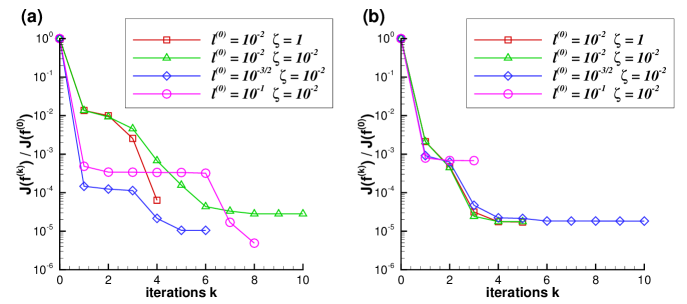
Figure 4: [Hill’s vortex] Decrease of cost functional ${\mathcal{J}}(f^{(k)})$ with $k$ for iterations starting with initial guess $f_{0}$ (a) underestimating and (b) overestimating the exact vorticity function (33). Different lines correspond to the values of $\ell^{(0)}$ and $\zeta$, cf. equation (28), indicated in the figure legends.

The histories of cost functional ${\mathcal{J}}(f^{(k)})$ with iterations corresponding to the two initial guesses are shown in Figures 4a and 4b, where we consider cases with different $\ell^{(0)}$ and $\zeta$ (cf. formula (28)). As discussed in Section 44.3, the values of the length-scale parameter $\ell^{(0)}\in[10^{-2},10^{-1}]$ are selected to lie within the range of variation of the streamfunction $\psi$ which in this problem is $[0,0.2]$. We note that in most cases the cost functional decreases by about five orders of magnitude over a few iterations. Reducing the length-scale $\ell^{(k)}$ with iterations has an effect on the rate of convergence when one initial guess is used, but appears to play little role when the other initial guess is employed. Hence, in this problem, we will adopt the values $\ell^{(0)}={10^{-1}}$ and $\zeta={10^{-1/5}}$. This choice of $\zeta$ ensures that $\ell^{(k)}$ decreases by an order of magnitude every five iterations, cf. (28).

In Figures 5a and 5b we show the optimal reconstructions $\hat{f}$ obtained in the two cases together with the corresponding initial guesses. We observe that in both cases the reconstructed vorticity function $\hat{f}$ is very close to the exact solution $C=1/2$ on the interval $[0,\psi_{\text{max}}]$, where $\psi_{\text{max}}=0.2$. In Figure 5b we note a slight deviation of the reconstructed vorticity function from the exact profile $f(\psi)=C=1/2$ for values of $\psi$ close to $\psi_{\text{max}}$. Given that the corresponding value of cost functional (11) is ${\mathcal{O}}(10^{-7})$, this provides evidence for a degree of ill-posedness of Problem 1, in the sense that finite modifications of the vorticity function $f$ have only a vanishing effect on the measurements appearing in (11). From the physical point of view, this behavior can be attributed to the fact that streamfunction values close to $\psi_{\text{max}}$ are attained on a small part of the domain $\Omega$ which is close to the centre of the vortex and therefore removed from the contour $\gamma_{0}$ where the measurements are acquired. If the goal is to maximize the reconstruction accuracy for values of $\psi$ close to $\psi_{\text{max}}$, this issue can be remedied by including additional measurements acquired within the vortex bubble $\Omega_{b}$ in cost functional ${\mathcal{J}}(f)$. As discussed in Section 44.1, the reconstruction method does allow for such a possibility.

The convergence of circulation $\Gamma$, impulse $I$ and energy $E$ with iterations $k$ to the values characterizing the exact solution is shown in Figures 6a and 6b for the two cases. In these figures we plot the relative error

$$\varepsilon^{(k)}(\Gamma):=\Bigg{|}\frac{\Gamma(f^{(k)})}{\Gamma_{\text{Hill}}}-1\Bigg{|}$$ (36)

for the vortex circulation and analogous expressions for the impulse and energy using logarithmic scale to determine the number of significant digits captured in the reconstruction. In the figures we note a fast, though nonmonotonous, convergence of the three diagnostic quantities to the corresponding exact values. We obtain approximately two digits of accuracy for the energy and three or more for the circulation and impulse.

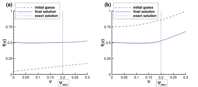
Figure 5: [Hill’s vortex] Reconstructed source functions $\hat{f}$ (blue solid lines) and the corresponding initial guesses (red dashed lines) when $f_{0}$ (a) underestimates and (b) overestimates the exact vorticity function (33). The black horizontal dotted line represents exact solution (33) with $a=2$ and $C=1/2$, whereas the vertical dotted lines mark the maximum value $\psi_{\text{max}}=0.2$ achieved by the streamfunction in exact solution.

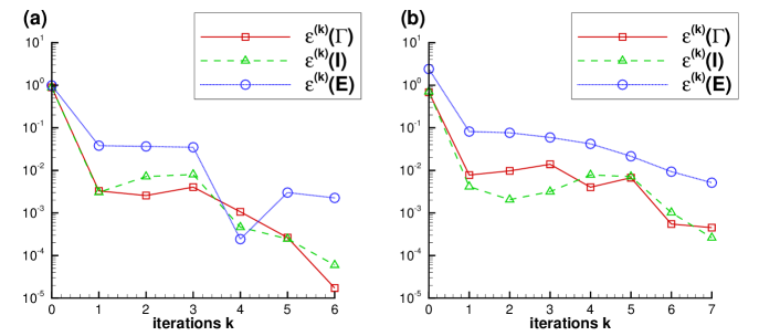
Figure 6: [Hill’s vortex] Evolution of the relative error $\varepsilon^{(k)}(\Gamma)$ for the circulation, cf. (36), and of analogously defined expressions for the impulse $I$ and energy $E$ showing convergence to the corresponding values $\Gamma_{\text{Hill}}$, $I_{\text{Hill}}$ and $E_{\text{Hill}}$ characterizing the exact solution, cf. (35). Iterations starting with initial guess $f_{0}$ underestimating and overestimating the exact vorticity function (33) are shown in panels (a) and (b), respectively.

7 Reconstruction of Vorticity from DNS Data

In this section we describe a more challenging task of reconstructing the vorticity function characterizing a realistic vortex ring. In the following we use a high-resolution DNS of the axisymmetric Navier-Stokes equations to generate a realistic evolution of a viscous vortex ring. The numerical approach is described in [14], although the data used in the present study corresponds to a higher Reynolds number and injection parameters chosen to reproduce the experiments reported in [55], see also [56]. The computational domain $(z,r)\in[0,10]\times[0,2]$ is discretized with $3200\times 800$ grid points ensuring convergence of the results. The vortex ring is generated by prescribing an appropriate axial velocity profile at the inlet section of the computational domain. We used the specified discharge velocity (SDV) model proposed in [56] to mimic the flow generated by a piston/cylinder mechanism pushing a column of fluid through a long pipe of diameter $D$. In the following, all presented quantities will be normalized using $D$ as the length scale and the maximum (piston) velocity $U_{0}$ at the entry of the pipe as the velocity scale. The corresponding reference time is thus $D/U_{0}$. The main physical parameter of the flow is the Reynolds number based on the characteristic velocity $Re_{D}={U_{0}\,D}/{\nu}=17,000$, with $\nu$ the viscosity of the fluid. Even at this elevated Reynolds number the vortex ring is known to remain laminar [33]. The injection is characterized by the stroke length ($L_{p}$) of the piston. We prescribed a piston velocity program used in actual experiments with $L_{p}/D=1.28$ [55].

For the reconstruction problem, we consider the vortex ring data obtained from the DNS at the nondimensional time $t=10$. This time instant corresponds to the post-formation phase, since the injection stopped at $t_{off}=2.26$. The DNS streamfunction $\psi_{\text{DNS}}{(z,r)}$ in the frame of reference moving with the vortex is computed by solving the general equation (5) within the rectangular domain used for the DNS together with the corresponding boundary conditions. We then use the level set $\psi_{\text{DNS}}=0$ to define the reconstruction domain $\Omega$ (see Figure 1b) and from this data extract the measurements $m=m(z,r)$ on $\gamma_{b}$ and $\gamma_{z}$, which serve as the target data in optimization problem (11)–(12). In the following, the velocity field is scaled by the translation velocity $W$ and distances are scaled by the vortex radius. The vortex centre is thus located at $(z,r)=(0,1)$ and $0\leq\psi_{\text{DNS}}\leq 0.791$.

7.1 Results of our reconstruction method

As a starting point, the empirical relation $\{\omega(z_{p},r_{p})/r_{p},\psi(z_{p},r_{p})\}_{p}$ between the vorticity and the streamfunction, cf. (1), at the points $(z_{p},r_{p})$ discretizing the flow domain $\Omega$ is shown as a scatter plot in Figures 7a,b. While these points tend to cluster along a rather well-defined curve, their local scattering is a manifestation of the fact that the original Navier-Stokes flow is viscous and not strictly steady in the chosen frame of reference. This scatter tends to increase for vortex rings with smaller Reynolds numbers. We now consider two approaches to reconstructing the vorticity function $f$ on the RHS in (8a) so that the inviscid vortex-ring model provides an accurate representation of the DNS data as quantified by the cost functional (11).

 

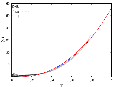
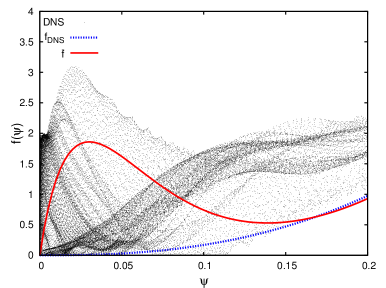
Figure 7: [DNS] Vorticity function $f(\psi)$ for (a) $\psi\in{\mathcal{I}}$ and (b) $\psi\in[0,0.2]$ (magnification of the region near the origin): (scatter plot with dots) relation $\{\omega(z_{p},r_{p})/r_{p},\psi(z_{p},r_{p})\}_{p}$ corresponding to discrete Navier-Stokes DNS data; (blue dotted line) least-squares fit $f_{DNS}$ given by (37) and (red solid line) the optimal reconstruction $\hat{f}$.

As the first approach we examine a least-squares fit of an empirical power-law relation for the vorticity function which yields

$$f_{\text{DNS}}(\psi)=56.337\,\psi^{2.520}.$$ (37)

We note that this relation has the property $f_{\text{DNS}}(0)=0$ ensuring that the vorticity support in the inviscid vortex-ring model coincides with $\Omega$. As is evident from Figure 7a, the fit captures the main trends exhibited by the data, except in the neighbourhood of the origin where the data reveals a larger scatter. On the other hand, due to its functional form the fit $f_{\text{DNS}}(\psi)$ approaches zero monotonously as $\psi\rightarrow 0$ (cf. Figure 7b). In addition, the empirical fit (37) also slightly misrepresents the slope $df/d\psi$. From the point of view of our reconstruction problem, the region characterized by small values of $\psi$ is particularly important, because it involves many data points in close proximity to the contour $\gamma_{0}$ on which the measurements are defined (this is reflected by a larger density of data points near the origin in Figures 7a,b). The values of the cost functional and the normalized errors in the reconstruction of the circulation, impulse and energy, cf. (9a)–(9c), corresponding to the empirical fit (37) are collected in Table 1.

	${\mathcal{J}}(f)$	$\Gamma$	$I$	$E$	$\omega_{\max}$
DNS		4.670	13.393	7.444	34.07
$f_{\text{DNS}}$	0.03263	4.212	13.002	7.470	32.17
$\hat{f}$	0.00315	4.607	13.385	6.900	29.19
Norbury-Fraenkel model	0.00864	4.671	13.974	7.448	14.45
Kaplanski-Rudi model	0.07939	3.898	12.288	6.647	30.43

Table 1: [DNS] Values of the cost functional (11), the diagnostic quantities (9) and the vorticity maximum $\omega_{\max}$ obtained for the empirical fit $f_{\text{DNS}}$ of the vorticity function, cf. (37), the optimally reconstructed vorticity function $\hat{f}$ and the fits with the Norbury-Fraenkel and Kaplanski-Rudi vortex-ring models (cf. Section 77.2).

As the second approach, we reconstruct the vorticity function optimally by solving Problem 1 as described above, with the least-squares fit (37) used as the initial guess in algorithm (16), i.e., $f_{0}=f_{\text{DNS}}$. As discussed in Section 44.3, in the absence of other relevant information, this fit will also be used to determine the behavior of the optimal reconstruction $\hat{f}(\psi)$ for limiting values of $\psi$. More precisely, in the reconstruction process we use the Sobolev gradients determined subject to the homogeneous Dirichlet boundary condition at $\psi=0$, cf. (27b), which together with our choice of the initial guess ensures that $\hat{f}(0)=0$. As regards large values $\psi>\max_{{\bf x}\in\Omega}\psi({\bf x})$, we will assume that the slope of $\hat{f}(\psi)$ will be given by the slope of the fit (37) which is ensured by the use of the homogeneous Neumann boundary condition (27c) at $\psi=\psi_{\text{max}}$. The characteristic length-scale in the inner product (10) was chosen as $\ell=10^{-3/2}\approx 0.0316$ and the decrement, cf. (28), as $\zeta=10^{1/5}$. The optimal vorticity function $\hat{f}(\psi)$ reconstructed in this way is shown in Figures 7a,b, whereas the corresponding values of the cost functional (11) and the diagnostic quantities (9) are indicated in Table 1. First of all, we observe that the reconstruction error as measured by the cost functional is reduced by an order of magnitude. This is achieved with an optimal vorticity function $\hat{f}(\psi)$ exhibiting a local maximum around $\psi=0.03$ which allows it to better match data points (more scattered for small $\psi$) and at the same time satisfy the constraint $\hat{f}(0)=0$. This is facilitated by our choice of the cost functional which is more sensitive to points in $\Omega$ characterized by small values of $\psi$ as they are located close to the boundary $\gamma_{0}$, cf. Figure 1. On the other hand, for larger values ($\psi\approx 0.8$), the optimal reconstruction reveals only a small improvement with respect to the empirical fit $f_{\text{DNS}}$. This is a consequence of the fact that parts of the flow domain with large values of $\psi$ are rather far from the contour $\gamma_{0}$ where the measurements are acquired. Given that the reconstruction errors represented by the cost functional ${\mathcal{J}}(f)$ are already very small, cf. Table 1, this effect can be attributed to the ill-posedness of the underlying inverse problem. As already discussed in Section 6, further improvements can be obtained using measurements distributed inside the vortex. As documented in Table 1, the optimal reconstruction improves the relative accuracy of both circulation and impulse by about one order of magnitude with respect to the model based on the empirical fit (37). On the other hand, the latter approach captures the energy and maximum vorticity (which are both nonlinear functions of the flow variables) more accurately than the optimal reconstruction.

7.2 Comparison with reconstruction methods based on analytical models

In this section we compare our results with more classical reconstruction approaches based on fits with analytical vortex-ring models. The approach directly related to our method relies on the Norbury-Fraenkel (NF) model for the steady inviscid vortex ring. It considers a constant vorticity function given by (2) and, once the vortex bubble was fixed, there are two parameters defining the vortex ring in this model: the vorticity intensity $C$ (i. e. $f(\psi)=C$) and the flux constant $k$ ($2\pi k$ represents the flow rate between the axis $0z$ and the boundary $\partial\Omega_{c}$, see Figure 1b). It was shown in [48] that, for a fixed vortex bubble, vortex-ring solutions exist if $C/k\geq\delta_{max}$, with $\delta_{max}$ estimated as a function of the first eigenvalue of the operator $\cal L$ on the bubble domain $\Omega$. If the vortex ring circulation is imposed, the solution is then unique and can be numerically calculated by an iterative algorithm suggested in [48]. In our case, corresponding to Figure 1, the fitting procedure gives the following values of the parameters: $C=13.39$ and $k=0.333$.

In the NF model, the vorticity distribution in the vortex core is linear, i. e. proportional to the distance from the symmetry axis (as in Hill’s spherical vortex model). This is not realistic, since a Gaussian vorticity distribution was reported in experimentally generated vortex rings [e. g. 30, 31]. This is remedied in the Kaplanski-Rudi (KR) vortex-ring model [6] which was derived as a linear first-order solution to the Navier-Stokes equation in the axisymmetric geometry and arbitrary times (see also [5]). The vorticity in the vortex core was predicted to be quasi-Gaussian, expressed by

$$\omega(z,r)=\frac{\Gamma_{0}}{\sqrt{2\pi}}\frac{\theta^{3}}{R_{0}^{2}}\exp\left[-\frac{1}{2}\left(\left(\frac{r}{L}\right)^{2}+\left(\frac{z}{L}\right)^{2}+\theta^{2}\right)\right]\textup{I}_{1}\left(\frac{r}{L}\theta\right),$$ (38)

where $\textup{I}_{1}$ is the modified Bessel function of the first kind, $L$ the effective viscous length scale of the vortex ring, $\Gamma_{0}$ the circulation of the vortex ring, $R_{0}$ its radius ($OC$ in Figure 1b) and $\theta=R_{0}/L$ a (viscous) parameter identifying the vortex. To use the KR model, we fit the DNS vorticity field with distribution (38) using the approximation $I_{1}(\eta)\approx\exp(\eta)/\sqrt{2\pi\eta}$ for large $\eta$. Under this approximation relation (38) becomes an isotropic 2D Gaussian. Using a non-linear fit with the BFGS minimization method we obtain the following values of the model parameters: $\Gamma_{0}=3.925$, $R_{0}=1.0047$, $L=0.142$, and $\theta=7.03$. We note that the fitted radius of the vortex ring is very close to the DNS value $R_{0}^{\text{DNS}}=1$ imposed by the adopted scaling (see Figure 1).

In our analysis we will focus on the vorticity fields of the different models as they exhibit more significant variation than the corresponding streamfunction fields. Vorticity contours for the DNS vortex ring and corresponding reconstructed fields are shown in Figure 8. For our optimal reconstruction, at each point $(z,r)$ the vorticity is computed as $\omega(z,r)=r\hat{f}(\psi(z,r))$ using cubic spline interpolation, cf. Section 55.1. The maximum values of the reconstructed vorticity $\omega_{\max}:=\max_{(z,r)\in\Omega}\omega(z,r)$ are given in table 1. They correspond to the vorticity at the centre of the vortex ring, except for the NF model in which $\omega(z,r)=Cr$. One can see that our model and the viscous KR model well approximate $\omega_{\max}$ from the DNS field. In Figure 8 it is also interesting to note that the prolate isocontour shapes in the DNS vorticity field are reproduced in our model. This is neither the case for the NF model (in which the vorticity isolines are described by $r=const$), nor for the viscous KR model (which features quasi-circular vorticity contours, as expected from formula (38) and its approximation by an isotropic Gaussian). As regards the KR model, we remark that this issue is remedied in its generalization proposed in [57], although it cannot be derived directly from the Navier-Stokes equation. The above observations are also corroborated by Figure 9 comparing the streamfunction and vorticity profiles along different directions in the DNS data and in the different vortex models. We note, in particular, that the vorticity profiles corresponding to the NF model are unrealistic.

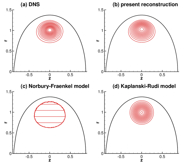
Figure 8: [DNS] Vorticity distribution inside the vortex ring bubble $\Omega$: (a) DNS, (b) $\omega(z,r)=r\hat{f}(\psi(z,r))$ with the optimal reconstruction $\hat{f}$ of the vorticity function and $\psi(z,r)$ obtained as the corresponding solution to problem (8), (c) fit with the Norbury-Fraenkel inviscid vortex-ring model, (d) fit with the Kaplanski-Rudi viscous vortex-ring model (38). Vorticity isocontours correspond to the values $\omega=2,4,\dots,32$.

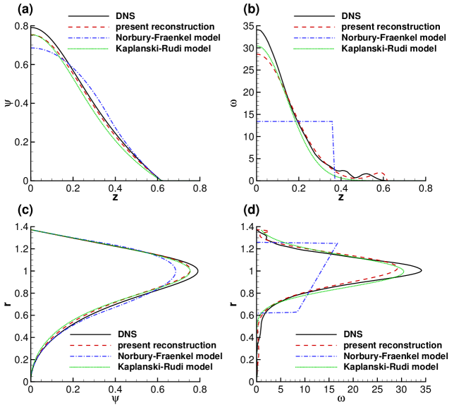
Figure 9: [DNS] Profiles of the streamfunction $\psi$ and vorticity $\omega$ through the centre of the vortex ring: (a,b) along the $z$-axis ($r=1,z>0$; note that the profiles are symmetric with respect to $z=0$) and (c, d) along the $r$-axis ($z=0$; see Figure 1b). Comparison between the DNS data (solid lines), our optimal reconstruction (dashed lines) and the fits with the inviscid Norbury-Fraenkel model (dash-dotted lines) and with the viscous Kaplanski-Rudi model (dotted lines).

Integral characteristics of the different vortex-ring models are collected in Table 1. It is interesting to note that the NF model, which is less physical in terms of its vorticity distribution, approximates the DNS values better than the other models. This explains why the NF model is often used to represent the integral characteristics of experimentally or numerically generated vortex rings (e. g. [27, 1]). The KR model gives the largest errors in the integral diagnostics because the fit used only the distribution of the vorticity, without imposing the circulation as in the case of the NF model.

The final comparison of the different models concerns the initial objective of the reconstruction procedure, namely, the representation of the tangential velocity $V_{t}=-{(1/r)}\partial\psi/\partial n$ on the boundary of the vortex bubble. These results are shown in Figure 10 which reveals a good agreement between the DNS data and the predictions of the proposed and the NF model. While the vortex model based on the optimal reconstruction of $f$ is more accurate along the boundary $\gamma_{b}$ of the vortex bubble, the NF model performs better on the axis $Oz$. In both cases the KR model underestimates the tangential velocity which is also reflected in the low circulation value it predicts (table 1).

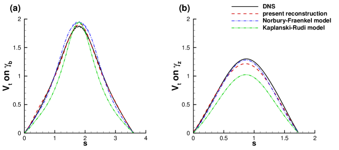
Figure 10: [DNS] Tangential velocity on the boundary segment (a) $\gamma_{b}$ (vortex bubble) and (b) $\gamma_{z}$ (along the $z$-axis) as a function of the arc-length coordinate $s$ along the boundary (see also Figure 1b for the definition of $\gamma_{b}$ and $\gamma_{z}$). Comparison between DNS data (solid lines), our optimal reconstruction (dashed lines), the fit with the inviscid Norbury-Fraenkel vortex ring model (dash-dot lines) and the fit with the Kaplanski-Rudi viscous vortex ring model (dotted lines).

We conclude that, while one of the analytic models may perform better with respect to a particular criterion (especially the ones used to determine its parameters), the proposed approach provides the most balanced and consistent representation with respect to all considered criteria. It must also be emphasized that our optimal reconstruction method uses information on the boundary ${\gamma_{b}\cup\gamma_{z}}$ of the vortex ring (see Figure 1b) only, while the reconstruction methods based on fits with the analytic vortex models used information in the entire domain $\Omega$.

8 Discussion, Conclusions and Outlook

In this study we have formulated and validated a novel solution approach to an inverse problem in vortex dynamics concerning the reconstruction of the vorticity function in 3D axisymmetric Euler flows. Solutions of such problems allow us to construct optimal inviscid vortex models for realistic flows. More generally, this is an example of the reconstruction of a nonlinear source term in an elliptic PDE and as such has many applications in fluid mechanics and beyond (more on this below). It also has some similarities to the “Calderon problem” which is one of the classical inverse problems studied in the context of elliptic PDEs. In particular, many questions concerning the uniqueness of the reconstructions remain open. In contrast to a number of earlier approaches which relied on finite-, and usually low-dimensional, parameterizations of the reconstructed vorticity function (e.g., [8]), the method proposed here is non-parametric and allows us to reconstruct the vorticity function in a very general form in which only the smoothness and boundary behavior are prescribed. A key element of the computational approach is a suitable reformulation of the adjoint-based optimization which was developed for the reconstruction of constitutive relations in [9, 10] and was already applied to other estimation problems in fluid mechanics in [11, 12].

In addition to standard tests on the accuracy of the adjoint gradients presented in Section 55.2, our approach was validated by reconstructing the vorticity functions in a classical problem involving Hill’s vortex. For benchmarking purposes, the inverse problem was set up using a smaller amount of measurement data than typically available in practice making the reconstruction more challenging. However, its accuracy was very good in terms of the terminal value of the cost functional (11), the optimal vorticity function $\hat{f}$ and the diagnostic quantities (9). The results obtained for the case with the actual DNS data in Section 7 demonstrated that the proposed approach can significantly improve the accuracy of the inviscid model as compared to a simple empirical fit. This is achieved by obtaining a more precise representation of the vorticity function for small values of $\psi$, made possible by the nonparametric form of the reconstruction approach.

A thorough comparison was also made between the vortex models developed here and the classical models of Norbury-Fraenkel and Kaplanski-Rudi. Although it is more costly from the computational point of view, the approach based on the optimal reconstruction of the vorticity function was shown to be superior in the sense that in addition to offering an accurate representation of the vorticity field inside the core and of the velocity on the boundary of the vortex bubble, it also captured the integral diagnostics with good accuracy. None of the analytic models was able to simultaneously achieve all of these objectives. It ought to be emphasized that our approach also required significantly less measurement data than the NF and KR models. This good performance is a result of an optimization formulation central to the proposed approach.

With encouraging results of the benchmark tests presented here, a natural research direction is to apply the proposed approach to DNS data and datasets obtained experimentally with techniques such as PIV over a broad range of Reynolds numbers. Measurement data available over larger parts of the flow domain should improve the robustness of reconstructions. The optimal reconstruction approach developed here will allow us to address the basic question how accurately actual viscous flows can be represented in terms of inviscid models of the type (8). In particular, one is interested in the fundamental limitations on the accuracy of such representations in terms of flow unsteadiness and finite viscosity effects. An aspect of the reconstruction problem which has not been addressed here, but which is likely to arise when using experimental data, is dealing with noisy measurements. This problem is however relatively well understood in the context of inverse problems [42].

9 Acknowledgements

The authors thank two referees for their helpful comments. They are also grateful to Dr. Vladislav Bukshtynov for sharing some of his software. B. P. acknowledges the generous hospitality of Laboratoire de mathématiques Raphaël Salem where this work was initiated in June 2013. He was also partially supported with an NSERC (Canada) Discovery Grant.

References

- Mohseni [2006] K. Mohseni. A formulation for calculating the translational velocity of a vortex ringor pair. Bioinspiration Biomimetics, 1:S57–S64, 2006.
- Dabiri [2009] J. O. Dabiri. Optimal vortex formation as a unifying principle in biological propulsion. Annual Review of Fluid Mechanics, 41(1):17–33, 2009.
- Begg et al. [2009] S. Begg, F. Kaplanski, S. Sazhin, M. Hindle, and M. Heikal. Vortex ring-like structures in gasoline fuel sprays under cold-start conditions. International Journal of Engine Research, 10(4):195–214, 2009.
- Kaplanski et al. [2010] F. Kaplanski, S. S. Sazhin, S. Begg, Y. Fukumoto, and M. Heikal. Dynamics of vortex rings and spray-induced vortex ring-like structures. European Journal of Mechanics B/Fluids, 29(3):208–216, 2010.
- Kaplanski and Rudi [1999] F. B. Kaplanski and Y. A. Rudi. Dynamics of a viscous vortex ring. Int. J. Fluid Mech. Res., 26:618–630, 1999.
- Kaplanski and Rudi [2005] F. B. Kaplanski and Y. A. Rudi. A model for the formation of "optimal" vortex ring taking into account viscosity. Phys. Fluids, 17:087101–087107, 2005.
- Fukumoto [2010] Y. Fukumoto. Global evolution of viscous vortex rings. Theoretical and Computational Fluid Dynamics, 24:335–347, 2010.
- Zhang and Danaila [2012] Y. Zhang and I. Danaila. A finite element BFGS algorithm for the reconstruction of the flow field generated by vortex rings. Journal of Numerical Mathematics, 20:325–340, 2012.
- Bukshtynov et al. [2011] V. Bukshtynov, O. Volkov, and B. Protas. On optimal reconstruction of constitutive relations. Physica D, 240:1228–1244, 2011.
- Bukshtynov and Protas [2013] V. Bukshtynov and B. Protas. Optimal reconstruction of material properties in complex multiphysics phenomena. J. Comp. Phys., 242:889–914, 2013.
- Protas et al. [2014] B. Protas, B. R. Noack, and M. Morzyński. An optimal model identification for oscillatory dynamics with a stable limit cycle. J. Nonlin. Sci., 24:245–275, 2014.
- Protas et al. [2015] B. Protas, B. R. Noack, and J. Östh. Optimal Nonlinear Eddy Viscosity in Galerkin Models of Turbulent Flows. Journal of Fluid Mechanics, 766:337–367, 2015.
- Isakov [1998] V. Isakov. Inverse Problems for Partial Differential Equations. Number 127 in Applied Mathematical Sciences. Springer, 1998.
- Danaila and Helie [2008] I. Danaila and J. Helie. Numerical simulation of the postformation evolution of a laminar vortex ring. Phys. Fluids, 20:073602, 2008.
- Batchelor [1988] G. K. Batchelor. An Introduction to Fluid Dynamics. Cambridge University Press, Cambridge, New York, 7th edition, 1988.
- Saffman [1992] P. G. Saffman. Vortex Dynamics. Cambridge University Press, Cambridge, New York, 1992.
- Hill [1894] M. J. M. Hill. On a spherical vortex. Philos. Trans. Roy. Soc. London, A185:213–245, 1894.
- Fraenkel and Berger [1974] L. E. Fraenkel and M. S. Berger. A global theory of steady vortex rings in an ideal fluid. Acta Math., 132:13–51, 1974.
- Ni [1980] W. M. Ni. On the existence of global vortex rings. J. d’Analyse Math., 37:208–247, 1980.
- Amick and Fraenkel [1988] C. J. Amick and L. E. Fraenkel. The uniqueness of a family of vortex rings. Arch. Rational Mech. Anal., 100:207–241, 1988.
- Amick and Fraenkel [1986] C. J. Amick and L. E. Fraenkel. The uniqueness of Hill’s spherical vortex. Arch. Rational Mech. Anal., 92:91–119, 1986.
- Norbury [1972] J. Norbury. A steady vortex ring close to Hill’s spherical vortex. Proc. Cambridge Phil. Soc., 72:253–282, 1972.
- Norbury [1973] J. Norbury. A family of steady vortex rings. J. Fluid Mech., 57:417–431, 1973.
- Fraenkel [1972] L. E. Fraenkel. Examples of steady vortex rings of small cross–section in an ideal fluid. J. Fluid Mech., 51:119, 1972.
- Moffatt [1969] H. K. Moffatt. The degree of knottedness of tangled vortex lines. J. Fluid Mech., 35:117–129, 1969.
- Elcrat et al. [2008] A. R. Elcrat, B. Fornberg, and K. G. Miller. Steady axisymmetric vortex flows with swirl and shear. J. Fluid Mech., 613:395–410, 2008.
- Mohseni and Gharib [1998] K. Mohseni and M. Gharib. A model for universal time scale of vortex ring formation. Phys. Fluids, 10:2436–2438, 1998.
- Shusser and Gharib [2000] M. Shusser and M. Gharib. Energy and velocity of a forming vortex ring. Phys. Fluids, 12:618, 2000.
- Linden and Turner [2001] P. F. Linden and J. S. Turner. The formation of ‘optimal’ vortex rings, and the effciency of propulsion devices. J. Fluid Mech., 427:61, 2001.
- Weigand and Gharib [1997] A. Weigand and M. Gharib. On the evolution of laminar vortex rings. Exp. Fluids, 22:447–457, 1997.
- Cater et al. [2004] J.E. Cater, J. Soria, and T.T. Lim. The interaction of the piston vortex with a piston-generated vortex ring. J. Fluid Mech., 499:327–343, 2004.
- Sullivan [1973] J. P. Sullivan. Study of a vortex ring using a laser doppler velocimeter. AIAA Journal, 11:1384, 1973.
- Akhmetov [2009] D. G. Akhmetov. Vortex Rings. Springer-Verlag, Berlin, Heidelberg, 2009.
- Prosperi et al. [2007] B. Prosperi, G. Delay, R. Bazile, J. Helie, and H.J. Nuglish. Fpiv study of gas entrainment by a hollow cone spray submitted to variable density. Experiments in Fluids, 43:315–327, 2007.
- Ambrosetti and Struwe [1989] A. Ambrosetti and M. Struwe. Existence of steady vortex rings in an ideal fluid. Arch. Rational Mech. Anal., 108(2):97–109, 1989.
- Esteban [1983] M. J. Esteban. Nonlinear elliptic problems in strip–like domains: symmetry of positive vortex rings. Nonlinear Analysis, Theory, Methods Applications, 7:365–379, 1983.
- Tadie [1994] Tadie. On the bifurcation of steady vortex rings from a Green function. Math. Proc. Camb. Phil. Soc., 116:555–568, 1994.
- Evans [2002] L. C. Evans. Partial Differential Equations. American Mathematical Society, 2002.
- Costa [2007] D. G. Costa. An Invitation to Variational Methods in Differential Equations. Birkhäuser, 2007.
- Nocedal and Wright [2002] J. Nocedal and S. Wright. Numerical Optimization. Springer, 2002.
- Luenberger [1969] D. Luenberger. Optimization by Vector Space Methods. John Wiley and Sons, 1969.
- Tarantola [2005] A. Tarantola. Inverse Problem Theory and Methods for Model Parameter Estimation. SIAM, 2005.
- Protas et al. [2004] B. Protas, T. Bewley, and G. Hagen. A comprehensive framework for the regularization of adjoint analysis in multiscale PDE systems. J. Comp. Phys., 195:49–89, 2004.
- Hecht et al. [2007] F. Hecht, O. Pironneau, A. Le Hyaric, and K. Ohtsuke. FreeFem++ (manual). www.freefem.org, 2007.
- Hecht [2012] F. Hecht. New developments in Freefem++. Journal of Numerical Mathematics, 20:251–266, 2012.
- Danaila and Kazemi [2010] I. Danaila and P. Kazemi. A new Sobolev gradient method for direct minimization of the Gross–Pitaevskii energy with rotation. SIAM J. Sci. Computing, 32:2447–2467, 2010.
- Danaila and Hecht [2010] I. Danaila and F. Hecht. A finite element method with mesh adaptivity for computing vortex states in fast-rotating Bose-Einstein condensates. J. Comput. Physics, 229:6946–6960, 2010.
- Zhang and Danaila [2013] Y. Zhang and I. Danaila. Existence and numerical modelling of vortex rings with elliptic boundaries. Applied Mathematical Modelling, 37:4809–4824, 2013.
- Danaila et al. [2014] I. Danaila, R. Moglan, F. Hecht, and S. Le Masson. A Newton method with adaptive finite elements for solving phase-change problems with natural convection. J. Comput. Physics, 274:826–840, 2014.
- Press et al. [1986] W. H. Press, B. P. Flanner, S. A. Teukolsky, and W. T. Vetterling. Numerical Recipes: the Art of Scientific Computations. Cambridge University Press, 1986.
- Homescu et al. [2002] C. Homescu, I. M. Navon, and Z. Li. Suppression of vortex shedding for flow around a circular cylinder using optimal control. Int. J. Numer. Meth. Fluids, 38:43–69, 2002.
- Gunzburger [2003] M. D. Gunzburger. Perspectives in Flow Control and Optimization. SIAM, 2003.
- Lamb [1932] H. Lamb. Hydrodynamics. Dover, New York, 1932.
- Marris and Aswani [1977] A. W. Marris and M. G. Aswani. On the general impossibility of controllable axi-symmetric Navier-Stokes motions. Archive for Rational Mechanics and Analysis, 63:107–153, 1977.
- Stewart et al. [2012] K. Stewart, C. Niebel, S. Jung, and P. Vlachos. The decay of confined vortex rings. Experiments in Fluids, 53:163–171, 2012.
- Danaila et al. [2009] I. Danaila, C. Vadean, and S. Danaila. Specified discharge velocity models for the numerical simulation of laminar vortex rings. Theor. Comput. Fluid Dynamics, 23:317–332, 2009.
- Fukumoto and Kaplanski [2008] Y. Fukumoto and F. B. Kaplanski. Global time evolution of an axisymmetric vortex ring at low reynolds numbers. Phys. Fluids, 20:053103, 2008.