A semi-flexible attracting-segment model of three-dimensional polymer collapse

Abstract

Recently it has been shown that a two-dimensional model of self-attracting polymers based on attracting segments with the addition of stiffness displays three phases: a swollen phase, a globular, liquid-like phase, and an anisotropic crystal-like phase. Here, we consider the attracting segment model in three dimensions with the addition of stiffness. While we again identify a swollen and two distinct collapsed phases, we find that both collapsed phases are anisotropic, so that there is no phase in which the polymer resembles a disordered liquid drop. Moreover all the phase transitions are first order.

1 Introduction

An isolated polymer in solution undergoes a collapse transition from a swollen coil to a collapsed globule as the temperature is lowered and consequently the quality of the solvent is reduced. The canonical lattice model used to describe this scenario is the model of Interacting Self-Avoiding Walks (ISAW) on a regular lattice, such as the square or simple cubic lattice [1, 2] .

At high temperatures the self-avoiding walk is swollen, in that the fractal dimension of the walk $d_{f}$ is less than the fractal dimension of simple random walks. The exponent $\nu=1/d_{f}$ describes the scaling of the size of the walk, as measured for example by its radius of gyration, as a function of the length of the walk. It is known that $\nu=3/4$ in two dimensions [3] and $\nu=0.587597(7)$ in three dimensions [4].

At low temperatures the self-avoiding walk is collapsed, in that the fractal dimension of the walk $d_{f}$ is equal to the dimension $d$ of the ambient space. The transition between the swollen coil and the collapsed globule happens at a particular temperature, called the $\theta$-temperature.

In the standard description of the coil-globule transition, the transition is a tricritical point related to the $N\rightarrow 0$ limit of the $\varphi^{4}$–$\varphi^{6}$ O($N$) field theory [5, 6, 7]; there is a second-order phase transition with a specific heat exponent conjectured to be $-1/3$ in two dimensions [8] and $0$ in three dimensions with a logarithmic divergence of the specific heat. In two dimensions the fractal dimension of the walk is expected to be $d_{f}=7/4$ [8] and $d_{f}=2$ with logarithmic corrections in three dimensions.

The canonical model of interacting self-avoiding walks fits this scenario. In this model one expects the low-temperature state to be a liquid drop, i.e., the polymer is compact but disordered.

In stark contrast to this scenario, there is another simple interacting polymer model, the Interacting Hydrogen-Bond model (IHB) [9, 10, 11], where a pair of sites on the self-avoiding walk acquires a hydrogen-like bond potential if the sites are (non-consecutive) nearest neighbours, as in the ISAW model, and each site lies on a straight section of the walk. This model has been introduced in the context of biopolymers where hydrogen bonding plays an important role [12]. In contrast to ISAW, this model displays a first-order collapse transition in both two and three dimensions. Here, the low-temperature state is an anisotropic compact phase described as a polymer crystal.

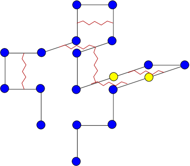
Figure 1: A self-avoiding walk with the interactions of the attracting segment (AS) model shown as intertwined curves between bonds of the walk on opposite sides of the squares of the lattice. Also shown is an example of a stiffness segment pair which obtains a stiffness energy in our generalisation.

Another model introduced to account for hydrogen bonding is the Attracting Segments model (AS) [13, 14, 15] (also known as ‘interacting bonds’). It is a lattice model based on self-avoiding walks where an attractive potential is assigned to bonds of the walk that lie adjacent and parallel on the lattice (though not consecutive along the walk), see Figure 1. On the square lattice, this model seems to have two phase transitions, one of which is identified as the $\theta$-point [15].

If one introduces stiffness into the ISAW model, one arrives at the semi-flexible ISAW model [16, 17, 18, 19]. In addition to the nearest-neighbour site interaction of ISAW, one introduces a stiffness energy associated with consecutive parallel bonds of the walk. This was studied on the cubic lattice by Bastolla and Grassberger [16], where it was shown that depending on the energetic weighting of straight segments one finds a single first-order transition from a swollen coil to a crystalline state for a strong energetic preference for straight segments, or a soft $\theta$-transition from a swollen coil to a liquid globule, followed by a first-order transition to a crystalline state. In two dimensions, a similar scenario has been found [20], the main difference being that the transition between the globule and the frozen state becomes second-order.

The semi-flexible AS model, in which both straight segments and interacting segments carry an energy, as shown in Figure 1, has been studied in two dimensions in [21], where it was found that it has a phase structure in common with the semi-flexible ISAW model.

In this paper, we discuss the semi-flexible AS model in three dimensions. While we again identify a swollen and two distinct collapsed phases, we find that both collapsed phases are anisotropic, so that there is no phase in which the polymer resembles a disordered liquid drop. The transitions between the swollen and each of the collapsed phases and between the two collapsed phases are first order. The three lines of transitions in parameter space meet at a triple point.

2 Our Study

2.1 Semi-flexible Attracting Segments model

Our semi-flexible attracting segments model (semi-flexible AS model) is a self-avoiding walk on the simple cubic lattice, with self-interactions as in the AS model [13, 14, 15] and a stiffness (or equivalently bend energy) added. Specifically, the energy of a single chain (walk) consists of two contributions (see Figure 1): the energy $-\varepsilon_{as}$ for each attracting segment pair, being a pair of occupied bonds of the lattice that are adjacent and parallel on the lattice and not consecutive along the walk; and an energy $-\varepsilon_{ss}$ for each stiffness segment pair, being a pair of bonds consecutive along the walk that are parallel. A walk configuration $\varphi_{n}$ of length $n$ has total energy

$$E_{n}(\varphi_{n})=-m_{as}(\varphi_{n})\ \varepsilon_{as}-m_{ss}(\varphi_{n})\ \varepsilon_{ss},$$ (2.1)

where $m_{as}$ denotes the number of attracting segment pairs and $m_{ss}$ denotes the number of stiffness segment pairs. The partition function is defined then as

$$Z_{n}(\beta_{as},\beta_{ss})=\sum_{m_{as},m_{ss}}C_{n,m_{as},m_{ss}}e^{\beta_{as}m_{as}+\beta_{ss}m_{ss}},$$ (2.2)

where $\beta_{as}=\varepsilon_{as}/k_{B}T$ and $\beta_{ss}=\varepsilon_{ss}/k_{B}T$ for temperature $T$ and Boltzmann constant $k_{B}$. The density of states, $C_{n,m_{as},m_{ss}}$, has been estimated by means of Monte Carlo simulations.

2.2 Simulations

On the cubic lattice we performed simulations using the FlatPERM algorithm [22], estimating the density of states up lengths for $n=128$ over the two parameters $m_{as}$ and $m_{ss}$. We use averages for the density of states from five independent runs. Moreover, we have simulated the density of states in $m_{as}$ at $\beta_{ss}=\pm 1.0$ and in $m_{ss}$ at $\beta_{as}=1.0$ for lengths up to $n=256$.

The density of states allows us to calculate the internal energy and the specific heat, or equivalently, the mean values and the fluctuations of $m_{as}$ and $m_{ss}$, respectively. This allows us to locate phase transitions through the possible divergences in the specific heat. To detect orientational order, we estimated an anisotropy parameter [16].

3 Results

3.1 Phase Diagram

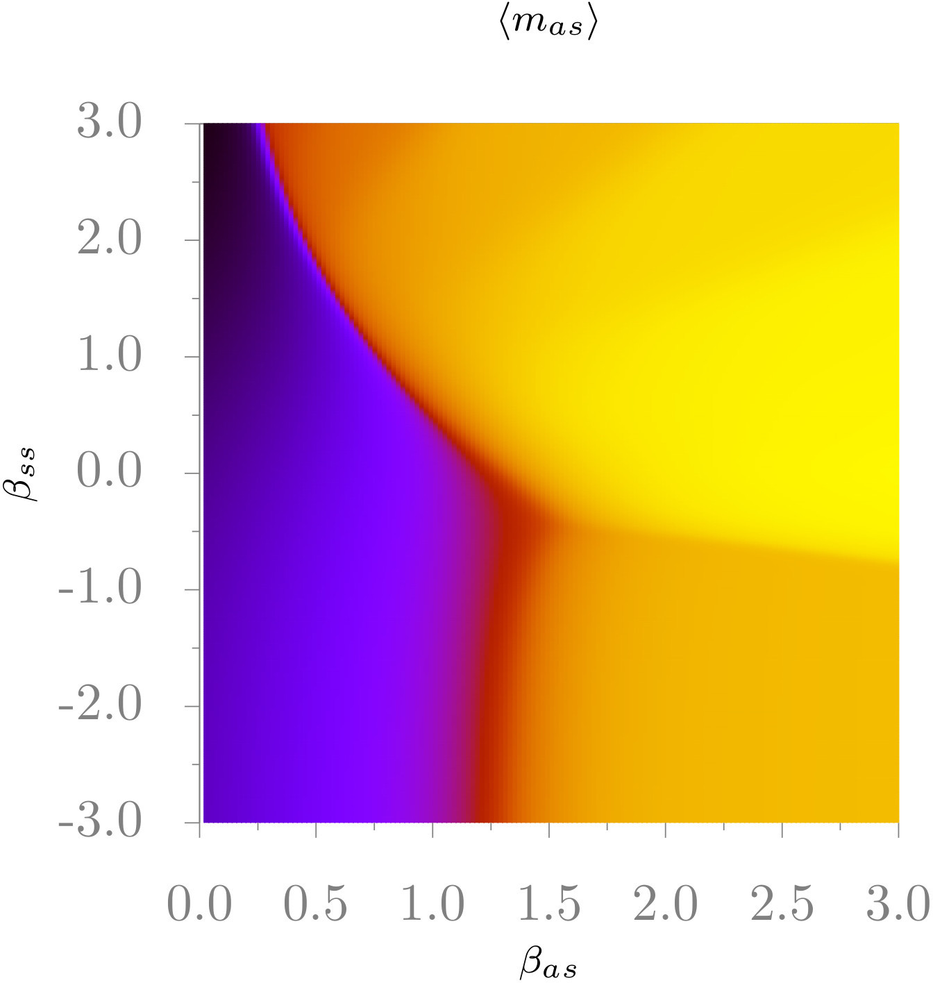
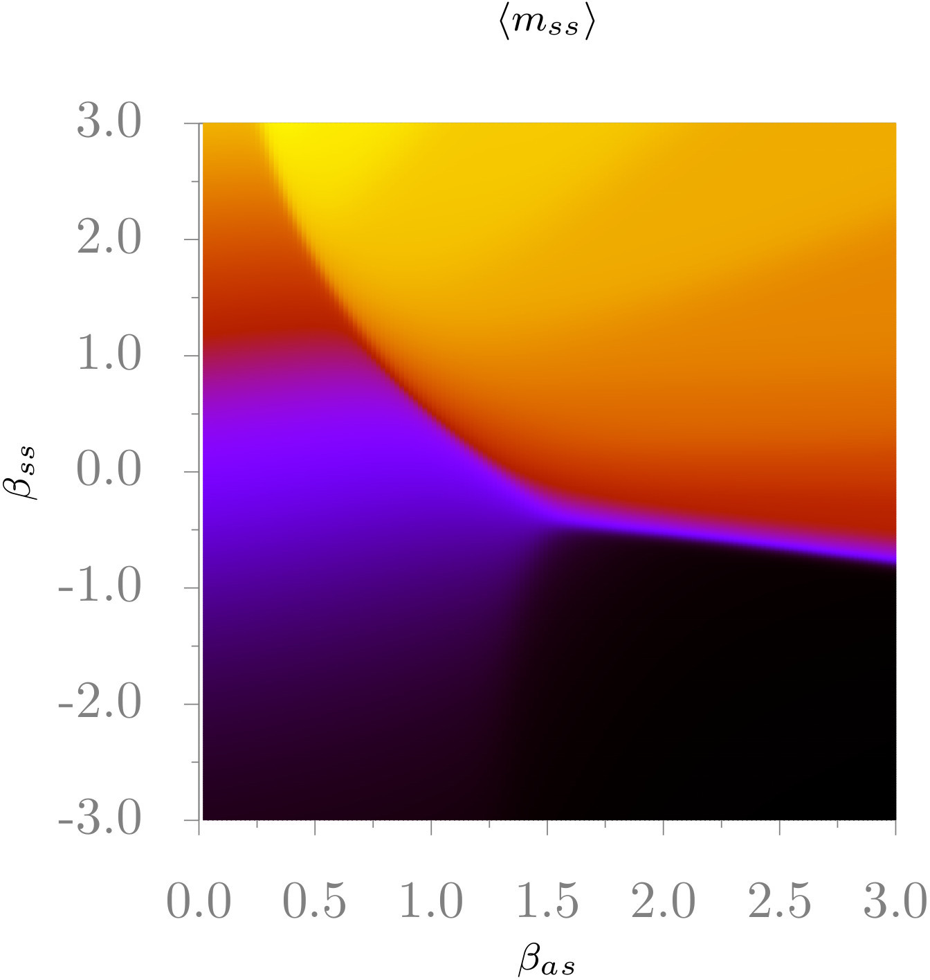
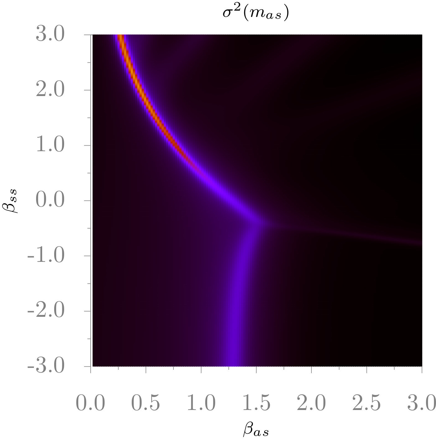
Figure 2: Expected value of the number of attracting segments pairs $m_{as}$ (top left) and stiff segment pairs $m_{ss}$ (top right) and their fluctuations $\sigma^{2}(m_{as})$ (bottom left) and $\sigma^{2}(m_{ss})$ (bottom right) for $128$-step walks as a function of $\beta_{as}$ and $\beta_{ss}$.

From the density of states for $128$-step walks, we compute the expected number of attracting segment pairs and stiff segment pairs, shown in Figure 2 as a function of $\beta_{as}$ and $\beta_{ss}$. There are three distinct regions recognisable. For small values of $\beta_{as}$ both $\langle m_{as}\rangle$ and $\langle m_{ss}\rangle$ are small, with $\langle m_{ss}\rangle$ increasing slowly as $\beta_{ss}$ increases. Upon increasing $\beta_{as}$, there is a sharp transition to large values of $\langle m_{as}\rangle$, indicative that the walks are collapsed on average. For large $\beta_{as}$ the density of straight segments, $\langle m_{ss}\rangle$, is small for negative values of $\beta_{ss}$, but increases sharply as $\beta_{ss}$ increases. This indicates that there are two distinct phases when $\beta_{as}$ is large (collapsed region).

Putting this broad information together it seems to indicate that there is a region in which the walk forms a swollen coil (the non-interacting SAW at $\beta_{as}=\beta_{ss}=0.0$ lies in this region), and that there are two regions in which the walk is collapsed. For one of the collapsed regions with negative $\beta_{ss}$, $\langle m_{as}\rangle$ is very small (in fact smaller than in the swollen region for the same values of $\beta_{as}$), whereas for the other collapsed region with positive $\beta_{ss}$, $\langle m_{as}\rangle$ is large.

The fluctuations $\sigma^{2}(m_{as})$ and $\sigma^{2}(m_{ss})$, also shown in Figure 2, confirm this scenario. The fluctuations of $m_{as}$ sharply peak upon increasing $\beta_{as}$. This peak is stronger for positive values of $\beta_{ss}$, where it is matched by a peak in the fluctuations of $m_{ss}$. For negative values, it is weaker, and there is no matching peak in the fluctuations of $m_{ss}$. This indicates that there are two different transitions from the swollen region to the collapsed region. Moreover, within the collapsed region we find a sharp peak in the fluctuations in $m_{ss}$ upon increasing $\beta_{ss}$, which is not matched by a peak in the fluctuations of $m_{as}$.

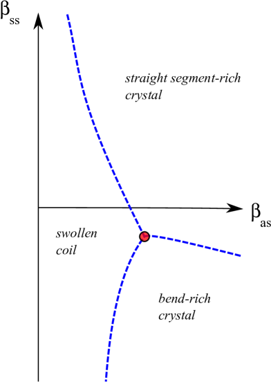
Figure 3: A sketch of the conjectured phase diagram, showing the swollen globular phase and the two crystalline phases. The three phase transition lines (dashed blue) are all first-order and meet in a common critical point (red).

We thus have three clearly defined regions in the $\beta_{as}$,$\beta_{ss}$-plane, delineated by rather sharp peaks in fluctuations. The presence of these fluctuations leads us to identify these regions with thermodynamic phases, so that we have a swollen globular phase, and two collapsed phases, one of which is rich in straight segments, and one of which is rich in bends. The conjectured phase diagram is shown in Figure 3. This phase diagram also indicates that the transition lines are first-order, and that the collapsed phases have in fact a crystalline structure. We will provide evidence for this in the next two sections.

3.2 Phase Transitions

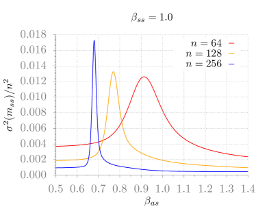
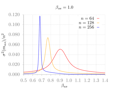
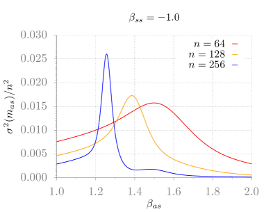
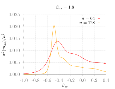
Figure 4: Scaled fluctuations in $m_{ss}$ and $m_{as}$ on the line $\beta_{ss}=1.0$ (top left and right, respectively), scaled fluctuations in $m_{as}$ on the line $\beta_{ss}=1.0$ (bottom left) and scaled fluctuations in $m_{ss}$ on the line $\beta_{as}=1.8$ (bottom right)

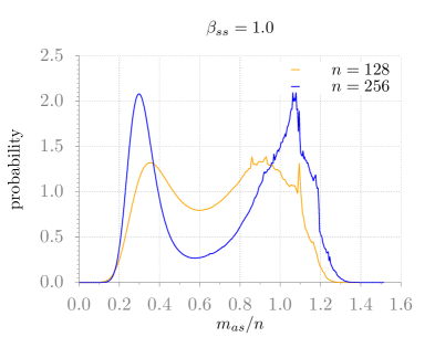
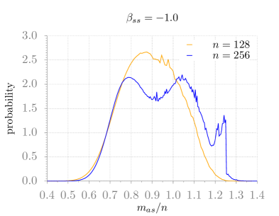
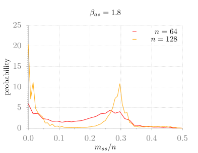
Figure 5: The top two figures show the scaled distributions of $m_{as}$ for $\beta_{ss}=1.0$ and $\beta_{ss}=-1.0$ (top left and right, respectively), for walk lengths $n=128$ and $n=256$, with the values of $\beta_{as}$ chosen such that the fluctuations in $m_{as}$ were maximal (for $\beta_{ss}=1.0$, $\beta_{as}=0.770$ and $0.681$ for $n=128$ and $256$, respectively, and for $\beta_{ss}=-1.0$, $\beta_{as}=1.382$ and $1.254$ for $n=128$ and $n=256$, respectively. The bottom figure shows the scaled distributions of $m_{ss}$ for $\beta_{as}=-1.8$ for walk lengths $n=64$ and $n=128$, with the values of $\beta_{ss}$ chosen such that the fluctuations in $m_{ss}$ were maximal ($\beta_{ss}=-0.420$ and $-0.487$ for $n=64$ and $n=128$, respectively).

In order to study the order of the three transitions, we consider the behaviour of the system on the straight lines $\beta_{ss}=1.0$, $\beta_{ss}=-1.0$, and $\beta_{as}=1.8$, which have been chosen to cut across the three different phase transition lines. In Figure 4 we show the scaled fluctuations $\sigma^{2}(m_{as})/n^{2}$ and $\sigma^{2}(m_{ss})/n^{2}$. The scaling has been chosen such that the peak height should tend to a constant if the transition is first-order. Clearly all three lines show strong transitions, and to clarify whether they are really first-order we consider the distribution of the appropriate microcanonical parameters.

In Figure 5 we show the distribution of $m_{as}$ at the peak of its fluctuation in $\beta_{as}$ along the lines $\beta_{ss}=1.0$ and $\beta_{ss}=-1.0$, and the distribution of $m_{ss}$ at the peak of its fluctuation in $\beta_{ss}$ along the line $\beta_{as}=1.8$. The distribution along $\beta_{ss}=1.0$ is clearly bimodal with the distance between the double peaks slightly widening as $n$ changes from $128$ to $256$. This confirms the first-order nature of that transition, and also explains why the fluctuation peak grows super-linearly in Figure 4. Along the line $\beta_{ss}=-1.0$ we also find an emerging double peak, albeit developing at much longer lengths. Finally, along the line $\beta_{as}=1.8$ we find a bimodal distribution with one peak located very closely to $m_{ss}=0$. Hence, we conclude that the transitions between all three phases are first-order.

3.3 Nature of the Collapsed Phases

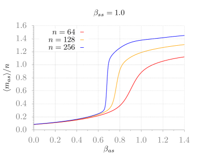
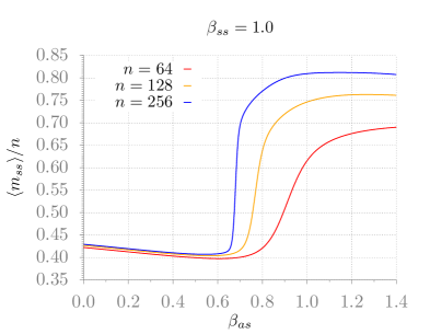
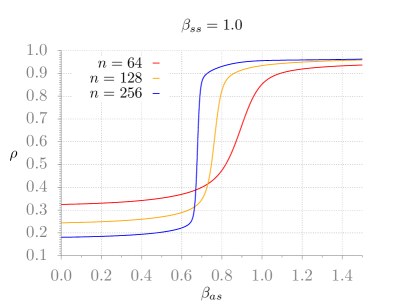
Figure 6: Line $\beta_{ss}=1.0$. The scaled number of contacts $\langle m_{as}\rangle$ and $\langle m_{ss}\rangle$ and anisotropy parameter as a function of $\beta_{as}$ for constant $\beta_{ss}=1.0$ for three system sizes $n=64,\;128$ and $256$.

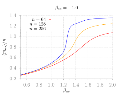
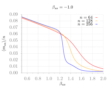
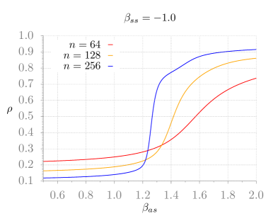
Figure 7: Line $\beta_{ss}=-1.0$. The scaled number of contacts $\langle m_{as}\rangle$ and $\langle m_{ss}\rangle$ and anisotropy parameter as a function of $\beta_{as}$ for constant $\beta_{ss}=-1.0$ for three system sizes $n=64,\;128$ and $256$.

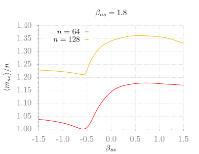
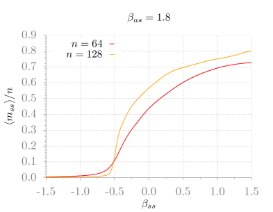
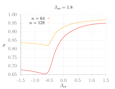
Figure 8: Line $\beta_{as}=1.8$. The scaled number of contacts $\langle m_{as}\rangle$ and $\langle m_{ss}\rangle$ and anisotropy parameter as a function of $\beta_{ss}$ for constant $\beta_{as}=1.8$ for two system sizes $n=64$ and $128$.

We now turn to the investigation of the two collapsed phases. As in [21], it will be helpful to consider an anisotropy parameter. In three dimensions, denoting the number of bonds parallel to the $x$-, $y$-, and $z$-axes by $n_{x}$, $n_{y}$, and $n_{z}$, respectively, we define

$$\rho=1.0-\frac{\min(n_{x},n_{y},n_{z})}{\max(n_{x},n_{y},n_{z})}$$ (3.1)

to be the anisotropy parameter. In a system without orientational order, this quantity tends to zero as the system size increases. A non-zero limiting value less than one of this quantity indicates weak orientational order with $n_{min}\propto n_{max}$, while a limiting value of one indicates strong orientational order, where $n_{max}\gg n_{min}$.

We first consider the change of the anisotropy parameter as the phase boundaries are crossed along the same three lines investigated earlier. This is shown in Figure 6 for $\beta_{ss}=1.0$, in Figure 7 for $\beta_{ss}=-1.0$, and in Figure 8 for $\beta_{as}=1.8$, together with the corresponding changes of the density of interacting segments $\langle m_{as}\rangle$ and straight segments $\langle m_{ss}\rangle$.

In addition to the change in $\langle m_{as}\rangle$ and $\langle m_{ss}\rangle$ described above, one sees that the anisotropy parameter decreases in the swollen phase, but jumps to a significantly larger value in the collapsed phases. There is a small difference in the value of the anisotropy parameter in both collapsed phases, but the change of $\rho$ as the length of the walk increases is such that $\rho$ might in fact tend to the same limiting value of one in the thermodynamic limit.

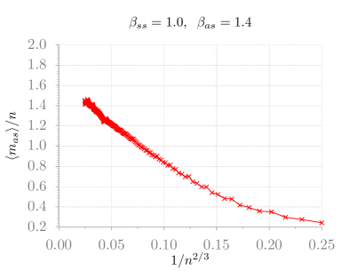
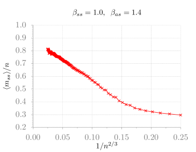
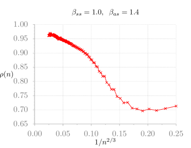
Figure 9: Number of contacts $\langle m_{ss}\rangle/n$ and $\langle m_{as}\rangle/n$ and anisotropy parameter, $\rho$, as function of the system size at $\beta_{as}=1.4$ and $\beta_{ss}=1.0$. Importantly, the anisotropy parameter, $\rho$, can be seen to converge to $\rho=1$ for infinite $n$ within error. The thermodynamic average of straight segments converges to a value near $0.9$ within error.

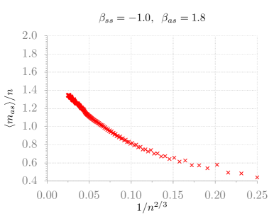
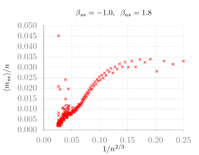
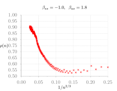
Figure 10: Number of contacts $\langle m_{ss}\rangle/n$ and $\langle m_{as}\rangle/n$ and anisotropy parameter, $\rho$, as function of the system size at $\beta_{as}=1.8$ and $\beta_{ss}=-1.0$. Importantly, the anisotropy parameter, $\rho$, can be seen to converge to $\rho=1$ for infinite $n$ within error and the thermodynamic average of straight segments converges to $\lim_{n\rightarrow\infty}\langle m_{ss}\rangle/n=0$ within error.

To test this, we now display the finite-size scaling behaviour at two points in the different collapsed phases. The values $\langle m_{ss}\rangle/n$, $\langle m_{as}\rangle/n$ and $\rho$ are shown as functions of $n^{-2/3}$ for $\beta_{as}=1.4$ and $\beta_{ss}=1.0$ in Figure 9 and for $\beta_{as}=1.8$ and $\beta_{ss}=-1.0$ in Figure 10. If the corrections to scaling are due to surface effects, one should find asymptotic straight lines as $n^{-2/3}$ tends to zero.

Both figures confirm the presence of $n^{-2/3}$-corrections, indicating a well-developed surface of the collapsed walk. The anisotropy parameter tends to one in both phases in the thermodynamic limit, indicating crystalline order. However, in one phase the density of straight segments tends to a limiting value close to one, whereas in the other phase this quantity tends to zero, showing clear evidence of two structurally very different crystalline structures, each of which has a different limiting density of attracting segments.

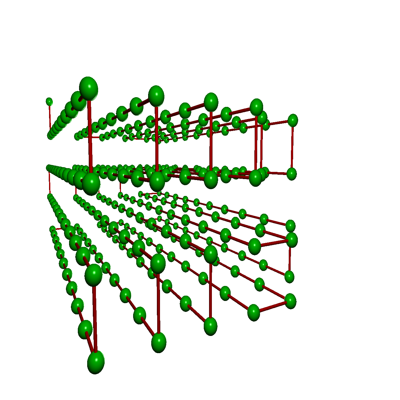
Figure 11: Typical configurations of length 128 at the parameter values $(\beta_{as},\beta_{ss})=(1.4,1.0)$ (left) and $(\beta_{as},\beta_{ss})=(1.8,-1.0)$ (right). The configuration on the left is an array of long straight lines of monomers while the configuration on the right contains mainly bends.

This scenario is confirmed by Figure 11, which shows typical configurations at these two parameter values: in the straight-rich phase, $(\beta_{as},\beta_{ss})=(1.4,1.0)$, the typical configurations consists of straight lines of monomers while in the bend rich phase, $(\beta_{as},\beta_{ss})=(1.8,-1.0)$, the typical configuration can be described as parallel sheets of two-dimensional configurations consisting only of bends. The limiting value of $\langle m_{as}\rangle/n$ is equal to $2$ in the former phase, and equal to $7/4$ in the latter phase, consistent with the numerical data shown in Figure 9 and Figure 10.

In this article we have discussed a three-dimensional semi-flexible AS model. We have characterised one swollen and two collapsed phases, and transition between them. In contrast to the two dimensional version of this model, both collapsed phases are anisotropic, and none of them resemble the disordered liquid drop.

References

- [1] W. J. C. Orr, Trans. Faraday Soc. 43, 12 (1947).
- [2] C. Vanderzande, A. L. Stella, and F. Seno, Phys. Rev. Lett. 67, 2757 (1991).
- [3] B. Nienhuis, Phys. Rev. Lett. 49, 1062 (1982).
- [4] N. Clisby, Phys. Rev. Lett. bf 104, 055702 (2010)
- [5] P.-G. de Gennes, J. Physique Lett. 36, L55 (1975).
- [6] M. J. Stephen, Phys. Lett. A. 53, 363 (1975).
- [7] B. Duplantier, J. Physique 43, 991 (1982).
- [8] B. Duplantier and H. Saleur, Phys. Rev. Lett. 59, 539 (1987).
- [9] J. Bascle, T. Garel, and H. Orland, J. Phys. II France 3, 245 (1993).
- [10] D. P. Foster and F. Seno, J. Phys. A. 34, 9939 (2001).
- [11] J. Krawczyk, A. L. Owczarek, T. Prellberg, and A. Rechnitzer, Phys. Rev. E , 051904:1 (2007).
- [12] L. Pauling and R. B. Corey, Proc. Nat. Acad. Sc. 37, 235, 251, 272, 729 (1951).
- [13] K. D. Machado, M. J.Oliveira, and J. F. Stilck, Phys. Rev. E 64, 051810 (2001).
- [14] C. Buzano and M. Pretti, J. Chem. Phys. 117, 10360 (2002).
- [15] D. P. Foster, J. Phys. A: Math. Theor. 40, 1963 (2007).
- [16] U. Bastolla and P. Grassberger, J. Stat. Phys. 89, 1061 (1997).
- [17] A. M. S. Lise and A. Pelizzola, Phys. Rev. E 58, R5241 (1998).
- [18] T. Vogel, M. Bachmann, and W. Janke, Phys. Rev. E 76, 061803 (2007).
- [19] J. P. K. Doye, R. P. Sear, and D. Frenkel, J. Chem. Phys. 108, 2134 (1997).
- [20] J. Krawczyk, A. L. Owczarek, and T. Prellberg, Physica A 388, 104 (2008).
- [21] J. Krawczyk, A. L. Owczarek, and T. Prellberg, Physica A 389, 1619 (2009).
- [22] T. Prellberg and J. Krawczyk, Phys. Rev. Lett. 92, 120602 (2004).