CNU-HEP-14-04, IPMU14-0344

Dark Matter in Split SUSY with Intermediate Higgses

Kingman Cheung^a,b,c, Ran Huo^d, Jae Sik Lee^e, Yue-Lin Sming Tsai^d

^a Department of Physics, National Tsing Hua University, Hsinchu 300, Taiwan
^b Division of Quantum Phases and Devices, School of Physics, Konkuk University, Seoul 143-701, Republic of Korea
^c Physics Division, National Center for Theoretical Sciences, Hsinchu, Taiwan
^d Kavli IPMU (WPI), The University of Tokyo, 5-1-5 Kashiwanoha, Kashiwa, Chiba 277-8583, Japan
^e Department of Physics, Chonnam National University, 300 Yongbong-dong, Buk-gu, Gwangju, 500-757, Republic of Korea
()

ABSTRACT

The searches for heavy Higgs bosons and supersymmetric (SUSY) particles at the LHC have left the minimal supersymmetric standard model (MSSM) with an unusual spectrum of SUSY particles, namely, all squarks are beyond a few TeV while the Higgs bosons other than the one observed at 125 GeV could be relatively light. In light of this, we study a scenario characterized by two scales: the SUSY breaking scale or the squark-mass scale $(M_{S})$ and the heavy Higgs-boson mass scale $(M_{A})$. We perform a survey of the MSSM parameter space with $M_{S}\raisebox{-3.69899pt}{~{}\shortstack{$<$ \\ [-0.07cm] $\sim$}}~{}10^{10}$ GeV and $M_{A}\raisebox{-3.69899pt}{~{}\shortstack{$<$ \\ [-0.07cm] $\sim$}}~{}10^{4}$ GeV such that the lightest Higgs boson mass is within the range of the observed Higgs boson as well as satisfying a number of constraints. The set of constraints include the invisible decay width of the $Z$ boson and that of the Higgs boson, the chargino-mass limit, dark matter relic abundance from Planck, the spin-independent cross section of direct detection by LUX, and gamma-ray flux from dwarf spheroidal galaxies and gamma-ray line constraints measured by Fermi LAT. Survived regions of parameter space feature the dark matter with correct relic abundance, which is achieved through either coannihilation with charginos, $A/H$ funnels, or both. We show that future measurements, e.g., XENON1T and LZ, of spin-independent cross sections can further squeeze the parameter space.

1 Introduction

Supersymmetry (SUSY) is one of the most elegant solutions, if not the best, to the gauge hierarchy problem. SUSY provides an efficient mechanism to break the electroweak symmetry dynamically with a large top Yukawa coupling. Another virtue is that the lightest SUSY particle (LSP) is automatically a dark matter (DM) candidate to satisfy the relic DM abundance assuming the $R$-parity conservation. The fine-tuning argument in the gauge hierarchy problem requires SUSY particles at work at the TeV scale to stabilize the gap between the electroweak scale and the grand unified theory (GUT) scale or the Planck scale. With this scale the gauge coupling unification is also naturally achieved in renormalization group equation (RGE) running.

Although SUSY has quite a number of merits at least theoretically, the biggest drawback of SUSY is that so far we have not observed any sign of SUSY. Nevertheless, we have observed a light standard model (SM) like Higgs boson, which is often a natural prediction of SUSY. The null results for all the searches of SUSY particles have pushed the mass scale of squarks beyond a few TeV [1]. While abandoning SUSY as a solution to the gauge hierarchy problem, such a high-scale SUSY scenario also draws more and more attention on CP problems [2], cosmological problems [3], and DM search [4]. On the other hand, the searches for the SUSY Higgs bosons provide the less stringent mass limits and it still seems possible to find them in the range of a few hundred GeV [5]. Consequently, we are left with an unusual spectrum of SUSY particles and Higgs bosons: (i) all squarks are heavy beyond a few TeV [1], (ii) the gluino is heavier than about 1 TeV [6], (iii) neutralinos and charginos can be of order $O(100-1000)$ GeV, (iv) heavy Higgs bosons can be of order $O(100-1000)$ GeV [5], and (v) a light Higgs boson with a mass $125$ GeV [7]. The spectrum is somewhat similar to the proposal of split SUSY [8], except that the heavy Higgs bosons need not be as heavy as those of split SUSY. We name the scenario the “modified split SUSY” framework, with two distinct scales: the SUSY breaking scale $M_{S}$ and the heavy Higgs-boson mass scale $M_{A}$. In the following, for simplicity we call this “modified split SUSY” as scenario A in which $M_{S}$ and $M_{A}$ are independent, while the original split SUSY as scenario B in which $M_{A}$ and $M_{S}$ are set to be equal. Since an extra TeV scale $M_{A}$ is obtained from cancellation of larger scales of $M_{S}$ or so, the fine tuning could be more serious than in the split SUSY.

We wish to be more specific and explicit about the framework and the motivation of our “modified split SUSY”. In the MSSM, the mass of the lightest neutral Higgs boson is basically determined by the weak gauge couplings and the vacuum expectation values of the neutral components of the two Higgs doublets and, accordingly, can not be much larger than the mass of the $Z$ boson. While the mass scale of the other 4 Higgs states cannot be fixed by requiring the electrowek symmetry breaking. Usually, the arbitrary mass parameter $M_{A}$ is introduced to fix the masses of the Higgs states other than the lightest one. Our notion is that there is no compelling reason for the scale $M_{A}$ to be equal to $M_{S}$ when we abandon SUSY as a solution to the hierarchy problem. With this choice of freedom we can modify the split SUSY (in split SUSY $M_{A}=M_{S}$) to have two independent parameters $M_{A}$ and $M_{S}$. With one more parameter, we can have more interesting collider and dark matter phenomenology, as well as more viable regions of parameter space, as we shall show in the main results. We, therefore, come with an interesting variety of the split SUSY. Instead of all the scalars being very heavy, we could have the $M_{A}$ much lighter than $M_{S}$. This will have profound effects on the dark matter phenomenology, especially the dark matter can annihilation via the near-resonance of the heavy Higgs bosons. Since the heavy Higgs bosons have much larger total decay widths than the light Higgs bosons, the resonance effect of the Higgs boson would enjoy much less fine tuning in giving the correct relic density of the dark matter. Thus, interesting parameter space regions become viable when $M_{A}$ goes down to sub-TeV and TeV ranges.

Phenomenologically, this modified split SUSY scenario is motivated by the possibility that the Higgs bosons other than the one observed at 125 GeV can be relatively light compared to the high SUSY scale $M_{S}$. If both $M_{A}$ and $M_{S}$ are set equal with $M_{A}<10\,\mathrm{TeV}$, as will be shown in Fig. 1, only a small region with large $\tan\beta$ is allowed. Nevertheless, if $M_{A}$ and $M_{S}$ are set at different values, much larger parameter space with a wide range of $\tan\beta$ will be allowed. With more parameter space we can then contrast it with other existing constraints. This is a strong motivation why we study this “modified split SUSY” scenario. We can then perform a careful analysis using all dark matter constraints and collider limits.

In this work, we consider the particle content of the minimal supersymmetric standard model (MSSM) in which the SUSY breaking scale or the sfermion-mass scale is denoted by $M_{S}$. The other scalar mass scale is the mass of heavy Higgs bosons characterized by $M_{A}$. In split SUSY, all sfermions and heavy scalar Higgs bosons are set a single scale $M_{S}$. However, in the modified split SUSY scenario under consideration, $M_{A}$ can be substantially smaller than $M_{S}$. The gauginos and Higgsinos have masses in hundred GeVs and TeV. The lightest neutralino, the dark matter candidate, will be composed of bino, wino, and Higgsino. In addition to the neutralino-chargino coannihilation region, we also have the near-resonance regions of the $Z$ boson, the light Higgs boson, as well as the heavy Higgs bosons, which is characterized by $M_{A}$. It is the latter that makes the scenario different from the conventional split SUSY. It is therefore important to explore this interesting scenario.

We perform a survey of the parameter space of the minimal supersymmetric standard model (MSSM) characterized by two scales: (i) the SUSY breaking scale $M_{S}$ with $M_{S}\raisebox{-3.69899pt}{~{}\shortstack{$<$ \\ [-0.07cm] $\sim$}}~{}10^{10}$ GeV, and (ii) the heavy Higgs-boson mass scale $(M_{A})$ with $M_{A}\raisebox{-3.69899pt}{~{}\shortstack{$<$ \\ [-0.07cm] $\sim$}}~{}10^{4}$ GeV, such that the lightest Higgs boson mass with large radiative corrections from heavy squarks is within the range of the mass of the observed Higgs boson. We choose $M_{A}$ smaller than or at most equal to $M_{S}$. Specifically, we assume the MSSM above the SUSY breaking scale $M_{S}$. Then we do the matching at the scale $M_{S}$ while we decouple all the sfermions. We evolve from $M_{S}$ down to $M_{A}$ with a set of RGEs comprising of two-Higgs doublet model (2HDM), gauge couplings, and gaugino couplings. For this purpose, we derive the RGEs governing the range between $M_{S}$ and $M_{A}$ and present them in Appendix A. Then we do the matching at the scale $M_{A}$ while we decouple all the heavy Higgs bosons. We evolve from $M_{A}$ down to the electroweak scale with a set of RGE comprising of the SM and the gauginos. The matching is then done at the electroweak scale. Once we obtain all the relevant parameters at the electroweak scale, we calculate all the observables and compare to experimental data.

In this work the LSP of the MSSM is the DM candidate, which is the lightest neutralino in the current scenario. Since we are strongly interested in DM, we include a number of other existing constraints on SUSY particles and DM:

1. the invisible decay width of the $Z$ boson and that of the Higgs boson,

2. the chargino-mass limit,

3. dark matter relic abundance from Planck,

4. the spin-independent cross section of direct detection by LUX, and

5. gamma-ray flux from dwarf spheroidal galaxies (dSphs) and gamma-ray line constraints measured by Fermi LAT.

Due to multidimensional model parameters involved in this work, it will be advantageous to adopt a Monte Carlo sampling technique to perform a global scan. In order to assess the robustness of our Monte Carlo results, we investigate both Bayesian maps in terms of marginal posterior (MP) and frequentist ones in terms of the profile likelihood (PL) technique. However, the likelihood functions of experimental constraints are the same for both approaches.

The organization is as follows. In the next section, we describe the theoretical framework of the modified split SUSY, including the matching conditions at the scales of $M_{S}$ and $M_{A}$, and the corresponding interactions of the particles involved. In Sec. 3, we list the set of constraints from collider and dark matter experiments that we use in this analysis. In Sec. 4, we present the results of our analysis using the methods of PL and MP. We discuss and conclude in Sec. 5.

2 Theoretical Framework

In the case under consideration, we have the two characteristic scales: the high SUSY scale $M_{S}$ and the Higgs mass scale $M_{A}$. The relevant phenomenology may be described by the effective Lagrangians depending on scale $Q$ as follows:

$$M_{S}<Q\hphantom{\,<M_{P}} : {\cal L}={\cal L}_{\rm MSSM}$$

$$M_{A}<Q<M_{S} : {\cal L}={\cal L}_{\rm 2HDM}+{\cal L}^{(1)}_{\tilde{\chi}}$$

$$\hphantom{M_{W}<}Q<M_{A} : {\cal L}={\cal L}_{\rm SM}+{\cal L}^{(2)}_{\tilde{\chi}}$$ (1)

2.1 Interactions for $M_{A}<Q<M_{S}$

At the scale $M_{S}$ all the sfermions decouple when we assume that they are heavier than or equal to the scale $M_{S}$. We are left with the spectrum of the Higgs sector of the 2HDM, gauginos, and higgsinos.

In this work, we take the general 2HDM potential as follows:

$$\mathrm{V}_{\rm 2HDM} = -\mu_{1}^{2}(\Phi_{1}^{\dagger}\Phi_{1})-\mu_{2}^{2}(\Phi_{2}^{\dagger}\Phi_{2})-m_{12}^{2}(\Phi_{1}^{\dagger}\Phi_{2})-m_{12}^{*2}(\Phi_{2}^{\dagger}\Phi_{1})$$ (2)

$$+\lambda_{1}(\Phi_{1}^{\dagger}\Phi_{1})^{2}+\lambda_{2}(\Phi_{2}^{\dagger}\Phi_{2})^{2}+2\lambda_{3}(\Phi_{1}^{\dagger}\Phi_{1})(\Phi_{2}^{\dagger}\Phi_{2})+2\lambda_{4}(\Phi_{1}^{\dagger}\Phi_{2})(\Phi_{2}^{\dagger}\Phi_{1})$$

$$+\lambda_{5}(\Phi_{1}^{\dagger}\Phi_{2})^{2}+\lambda_{5}^{*}(\Phi_{2}^{\dagger}\Phi_{1})^{2}+2\lambda_{6}(\Phi_{1}^{\dagger}\Phi_{1})(\Phi_{1}^{\dagger}\Phi_{2})+2\lambda_{6}^{*}(\Phi_{1}^{\dagger}\Phi_{1})(\Phi_{2}^{\dagger}\Phi_{1})$$

$$+2\lambda_{7}(\Phi_{2}^{\dagger}\Phi_{2})(\Phi_{1}^{\dagger}\Phi_{2})+2\lambda_{7}^{*}(\Phi_{2}^{\dagger}\Phi_{2})(\Phi_{2}^{\dagger}\Phi_{1})$$

with the parameterization

$$\Phi_{1} = -i\sigma_{2}\,H_{d}^{*}=\left(\begin{array}[]{cc}0&-1\\ 1&0\end{array}\right)\,\left(\begin{array}[]{c}\frac{1}{\sqrt{2}}\,(v_{d}+H_{d}^{0}-iA_{d}^{0})\\ -H_{d}^{-}\end{array}\right)^{*}=\left(\begin{array}[]{c}H_{d}^{+}\\ \frac{1}{\sqrt{2}}\,(v_{d}+H_{d}^{0}+iA_{d}^{0})\end{array}\right)\,;\ \ \$$ (9)

$$\Phi_{2} = H_{u}=\left(\begin{array}[]{c}H_{u}^{+}\\ \frac{1}{\sqrt{2}}\,(v_{u}+H_{u}^{0}+iA_{u}^{0})\end{array}\right)\,;\ \ \$$ (12)

and $v_{d}=v\cos\beta=vc_{\beta}$, $v_{u}=v\sin\beta=vs_{\beta}$, and $v\simeq 245$ GeV. Then we have

$$M_{A}^{2} = M_{H^{\pm}}^{2}+\lambda_{4}v^{2}-\Re{\rm e}(\lambda_{5})v^{2}\,,$$ (13)

$$M_{H^{\pm}}^{2} = \frac{\Re{\rm e}(m_{12}^{2})}{c_{\beta}s_{\beta}}-\frac{v^{2}}{c_{\beta}s_{\beta}}\left[\lambda_{4}c_{\beta}s_{\beta}+c_{\beta}s_{\beta}\Re{\rm e}(\lambda_{5})+c_{\beta}^{2}\Re{\rm e}(\lambda_{6})+s_{\beta}^{2}\Re{\rm e}(\lambda_{7})\right]\,,$$

where $A=-s_{\beta}A_{d}^{0}+c_{\beta}A_{u}^{0}$ and $H^{+}=-s_{\beta}H_{d}^{+}+c_{\beta}H_{u}^{+}$.

The wino(bino)-Higgsino-Higgs interactions are given by

$${\cal L}_{\tilde{\chi}}^{(1)} = \frac{1}{\sqrt{2}}H_{u}^{\dagger}\left(\tilde{g}_{u}\sigma^{a}\widetilde{W}^{a}+\tilde{g}_{u}^{\prime}\widetilde{B}\right)\,\widetilde{H}_{u}$$ (14)

$$+ \frac{1}{\sqrt{2}}H_{d}^{\dagger}\left(\tilde{g}_{d}\sigma^{a}\widetilde{W}^{a}-\tilde{g}_{d}^{\prime}\widetilde{B}\right)\,\widetilde{H}_{d}\ +\ {\rm h.c.}\,$$

where $\sigma^{a}$ are the Pauli matrices. We note $H_{d}^{\dagger}=-\Phi_{1}^{T}\,i\sigma_{2}=\left(\frac{1}{\sqrt{2}}\,(v_{d}+H_{d}^{0}+iA_{d}^{0}),-H_{d}^{+}\right)$.

2.2 Matching at $M_{S}$

The couplings of the interactions when $M_{A}<Q<M_{S}$ are determined by the matching conditions at $M_{S}$ and the RGE evolution from $M_{S}$ to $Q$. Assuming that all the sfermions are degenerate at $M_{S}$, the quartic couplings at the scale $M_{S}$ are given by

$$\lambda_{1} = \frac{1}{8}(g^{2}+g^{\prime 2})+\frac{N_{c}}{(4\pi)^{2}}\bigg{(}y_{b}^{4}\frac{A_{b}^{2}}{M_{S}^{2}}(1-\frac{A_{b}^{2}}{12M_{S}^{2}})-y_{t}^{4}\frac{\mu^{4}}{12M_{S}^{4}}\bigg{)}$$

$$\lambda_{2} = \frac{1}{8}(g^{2}+g^{\prime 2})+\frac{N_{c}}{(4\pi)^{2}}\bigg{(}y_{t}^{4}\frac{A_{t}^{2}}{M_{S}^{2}}(1-\frac{A_{t}^{2}}{12M_{S}^{2}})-y_{b}^{4}\frac{\mu^{4}}{12M_{S}^{4}}\bigg{)}$$

$$\lambda_{3} = \frac{1}{8}(g^{2}-g^{\prime 2})+\frac{N_{c}}{(4\pi)^{2}}\bigg{(}y_{b}^{2}y_{t}^{2}\frac{A_{tb}}{2}+y_{t}^{4}(\frac{\mu^{2}}{4M_{S}^{2}}-\frac{\mu^{2}A_{t}^{2}}{12M_{S}^{4}})+y_{b}^{4}(\frac{\mu^{2}}{4M_{S}^{2}}-\frac{\mu^{2}A_{b}^{2}}{12M_{S}^{4}})\bigg{)}$$

$$\lambda_{4} = -\frac{1}{4}g^{2}+\frac{N_{c}}{(4\pi)^{2}}\bigg{(}-y_{b}^{2}y_{t}^{2}\frac{A_{tb}}{2}+y_{t}^{4}(\frac{\mu^{2}}{4M_{S}^{2}}-\frac{\mu^{2}A_{t}^{2}}{12M_{S}^{4}})+y_{b}^{4}(\frac{\mu^{2}}{4M_{S}^{2}}-\frac{\mu^{2}A_{b}^{2}}{12M_{S}^{4}})\bigg{)}$$

$$\lambda_{5} = -\frac{N_{c}}{(4\pi)^{2}}\bigg{(}y_{t}^{4}\frac{\mu^{2}A_{t}^{2}}{12M_{S}^{4}}+y_{b}^{4}\frac{\mu^{2}A_{b}^{2}}{12M_{S}^{4}}\bigg{)},$$

$$\lambda_{6} = \frac{N_{c}}{(4\pi)^{2}}\bigg{(}y_{b}^{4}\frac{\mu A_{b}}{M_{S}^{2}}(-\frac{1}{2}+\frac{A_{b}^{2}}{12M_{S}^{2}})+y_{t}^{4}\frac{\mu^{3}A_{t}}{12M_{S}^{4}}\bigg{)},$$

$$\lambda_{7} = \frac{N_{c}}{(4\pi)^{2}}\bigg{(}y_{t}^{4}\frac{\mu A_{t}}{M_{S}^{2}}(-\frac{1}{2}+\frac{A_{t}^{2}}{12M_{S}^{2}})+y_{b}^{4}\frac{\mu^{3}A_{b}}{12M_{S}^{4}}\bigg{)},$$ (15)

with

$$A_{tb}=\frac{1}{6}\bigg{(}-\frac{6\mu^{2}}{M_{S}^{2}}-\frac{(\mu^{2}-A_{b}A_{t})^{2}}{M_{S}^{4}}+\frac{3(A_{b}+A_{t})^{2}}{M_{S}^{2}}\bigg{)}\,.$$ (16)

We note that the quartic couplings at $M_{S}$ consist of its tree level values and the threshold corrections induced by the $A$ and $\mu$ terms. We further observe $\lambda_{5,6,7}$ vanish without including the threshold corrections.

On the other hand, for the wino(bino)-Higgsino-Higgs couplings at the scale $M_{S}$, we have

$$\tilde{g}^{(\prime)}_{u}=\tilde{g}^{(\prime)}_{d}=g^{(\prime)}\,.$$ (17)

We note the relation $g^{\prime}=\sqrt{3/5}\,g_{1}$.

The threshold corrections to the gauge and Yukawa couplings at $M_{S}$ also vanish in the framework under consideration or when all the sfermions are degenerate at $M_{S}$.

2.3 Interactions for $Q<M_{A}$

When the scale drops below $M_{A}$, all the heavy Higgs bosons decouple. We are left with the SM particles, a light Higgs boson, gauginos, and higgsinos.

The SM Higgs potential is given by

$$V_{\rm SM}=\lambda\left[(\Phi^{\dagger}\Phi)^{2}-\frac{v^{2}}{2}\right]^{2}$$ (18)

with

$$\Phi=\left(\begin{array}[]{c}G^{+}\\ \frac{1}{\sqrt{2}}\,(v+h+iG^{0})\end{array}\right)\,$$ (19)

where $G^{\pm,0}$ denotes the would-be Goldstone bosons and $h$ the physical neutral Higgs state. We note $m_{h}^{2}=2\lambda v^{2}$. The wino(bino)-Higgsino-Higgs interactions are then given by

$${\cal L}_{\tilde{\chi}}^{(2)} = \frac{1}{\sqrt{2}}\Phi^{\dagger}\left(\hat{g}_{u}\sigma^{a}\widetilde{W}^{a}+\hat{g}_{u}^{\prime}\widetilde{B}\right)\,\widetilde{H}_{u}$$ (20)

$$+ \frac{1}{\sqrt{2}}(-\Phi^{T}\,i\sigma_{2})\left(\hat{g}_{d}\sigma^{a}\widetilde{W}^{a}-\hat{g}_{d}^{\prime}\widetilde{B}\right)\,\widetilde{H}_{d}\ +\ {\rm h.c.}\,.$$

2.4 Matching at $M_{A}$

The couplings of the interactions when $Q<M_{A}$ are determined by the matching conditions at $M_{A}$ and the RGE evolution from $M_{A}$ to $Q$.

At the scale $M_{A}$, the quartic coupling $\lambda$ of the SM Higgs potential is given by

$$\lambda = \lambda_{1}\cos^{4}\beta+\lambda_{2}\sin^{4}\beta+2\tilde{\lambda}_{3}\cos^{2}\beta\sin^{2}\beta$$ (21)

$$+ 4\lambda_{6}\cos^{3}\beta\sin\beta+4\lambda_{7}\cos\beta\sin^{3}\beta+\delta\lambda$$

where $\tilde{\lambda}_{3}=\lambda_{3}+\lambda_{4}+\lambda_{5}$ and $\delta\lambda$ denotes the threshold correction. We find that the threshold correction to $\lambda$ is given by

$$\delta\lambda = \frac{1}{4\pi^{2}}\bigg{[}\left(\lambda_{A}^{3}\frac{v^{2}}{M_{A}^{2}}-\frac{1}{3}\lambda_{A}^{4}\frac{v^{4}}{M_{A}^{4}}\right)+\left(\lambda_{H}^{3}\frac{v^{2}}{M_{H}^{2}}-\frac{1}{3}\lambda_{H}^{4}\frac{v^{4}}{M_{H}^{4}}\right)+2\left(\lambda_{\pm}^{3}\frac{v^{2}}{M_{H^{\pm}}^{2}}-\frac{1}{3}\lambda_{\pm}^{4}\frac{v^{4}}{M_{H^{\pm}}^{4}}\right)\bigg{]}$$ (22)

$$+ \frac{1}{8\pi^{2}}\left(\lambda_{H}^{2}\ln\frac{M_{H}}{M_{A}}+2\lambda_{\pm}^{2}\ln\frac{M_{H^{\pm}}}{M_{A}}\right)$$

where $M_{H}$ denotes the mass of the heavier CP-even neutral Higgs boson and the couplings $\lambda_{A,H,\pm}$ are defined as follows:

$$\lambda_{A} = (\lambda_{3}+\lambda_{4}-\lambda_{5})+(\lambda_{1}+\lambda_{2}-2\tilde{\lambda}_{3})\cos^{2}\beta\sin^{2}\beta+(-\lambda_{6}+\lambda_{7})\sin 2\beta\cos 2\beta\,,$$

$$\lambda_{H} = \tilde{\lambda}_{3}+3(\lambda_{1}+\lambda_{2}-2\tilde{\lambda}_{3})\cos^{2}\beta\sin^{2}\beta+3(-\lambda_{6}+\lambda_{7})\sin 2\beta\cos 2\beta\,,$$

$$\lambda_{\pm} = \lambda_{3}+(\lambda_{1}+\lambda_{2}-2\tilde{\lambda}_{3})\cos^{2}\beta\sin^{2}\beta+(-\lambda_{6}+\lambda_{7})\sin 2\beta\cos 2\beta.$$ (23)

The wino(bino)-Higgsino-Higgs couplings at $M_{A}$ are given by

$$\hat{g}^{(\prime)}_{u}=\tilde{g}^{(\prime)}\,\sin\beta\,;\ \ \ \hat{g}^{(\prime)}_{d}=\tilde{g}^{(\prime)}\,\cos\beta\,.$$ (24)

The threshold corrections to the gauge and Yukawa couplings at $M_{A}$ are neglected because of the approximated degeneracy among $M_{A}$, $M_{H}$, and $M_{H^{\pm}}$.

2.5 Matching at the electroweak scale

Matching at the electroweak scale is exactly the same as in the original split SUSY framework. We closely follow Ref. [9] to include the threshold corrections to the gauge couplings at the electroweak scale and to calculate the pole masses for the Higgs boson and the top quark.

Since we are adopting the one-loop matching conditions, see Eqs. (15) and (21), it is more appropriate to employ two-loop RGEs. However, not all the two-loop RGEs are available for the present framework, and the higher-order corrections may be minimized by the judicious choice of the top-quark mass for the scale where the lightest Higgs mass is estimated. Our approach is to be considered as an intermediate step towards the more precise calculation of the lightest Higgs mass in our modified split SUSY scenario.

3 Experimental Constraints and Likelihoods

In this section, we describe how to construct the likelihood functions involved with experimental constraints which are used in both MP and PL approaches. For the experimental constraints considered in this work, we assume either half-Gaussian or Gaussian distribution when the central values $\mu$, experimental errors $\sigma$, and theoretical errors $\tau$ are available. Otherwise, we take Poisson distributions.

In Table 1, in the second last column, we show the likelihoods of each experimental constraint. Here “hard cut” means we apply the 95% upper limits instead of constructing its likelihood. For the details of our statistical treatment, we refer to Appendix B. In the following subsections, we give more details of the constraint and likelihood of each measurement.

Measurement	central value $\mu$	Error: ($\sigma$, $\tau$)	Distribution	Ref.
$\Gamma_{\rm{inv}}^{Z}$	$499\,{\rm MeV}$	$1.5\,{\rm MeV},0.0$	Gaussian	[10]
$\Gamma_{\rm{inv}}^{h}$	$0.1\,{\rm MeV}$	${}^{+0.51}_{-0.41}\,{\rm MeV},0.0$	Gaussian	[11]
$m_{\chi^{\pm}}$	$103.5\,{\rm GeV}$	$0.0\,{\rm GeV},1\%$	half-Gaussian	[12]
relic abundance	$0.1186$	$0.0031$, $10\%$	half-Gaussian	[13]
LUX (2013)	see Ref. [14]	see Ref. [14]	Poisson	[15]
dSphs $\gamma$-ray	see Ref. [16]	see Ref. [16]	Poisson	[17]
Monochromatic $Z^{0}\gamma$ and $\gamma\gamma$	95% upper limits	95% upper limits	hard-cut	[18]

Table 1: The experimental constraints and the likelihoods. Where it is applicable, the central value $\mu$, experimental error $\sigma$, and theoretical error $\tau$ are given.

3.1 Colliders

3.1.1 Invisible decay widths

The invisible decay width of the $Z$ boson was accurately measured by taking the difference between the total width and the visible width, and is well explained by the three light active neutrino species of the SM. Any additional invisible decays of the $Z$ boson are strongly constrained by this data. In the current framework, the additional invisible width comes from $Z\to\chi^{0}_{1}\chi^{0}_{1}$. With the invisible width given in the PDG [10], $\Gamma^{Z}_{inv}=499\pm 1.5$ MeV, we can constrain $Z\to\chi^{0}_{1}\chi^{0}_{1}$.

If the neutralino mass is below $m_{h}/2$, the Higgs boson can decay into a pair of neutralinos, thus contributing to an invisible width of the Higgs boson. From a global fit using the Higgs-boson data at the 7 and 8 TeV runs of the LHC, the invisible width of the Higgs boson is constrained to be $\Gamma^{h}_{\rm inv}<0.6$ MeV [11] at 1-$\sigma$ level if all other parameters are fixed at their SM values. If other parameters are allowed to vary, the $\Gamma^{h}_{\rm inv}$ would have a more relaxed limit, which is about the same as the bound from the direct search on the invisible mode of the Higgs boson, which has a branching ratio about $50\%$ [19]. Nevertheless, we use $\Gamma^{h}_{\rm inv}<0.6$ MeV in this work, as shown in Table 1.

3.1.2 Chargino mass

The mass limits on charginos come either from direct search or indirectly from the constraint set by the non-observation of ${\chi}^{0}_{2}$ states on the gaugino and higgsino MSSM parameters $M_{2}$ and $\mu$. For generic values of the MSSM parameters, limits from high-energy $e^{+}e^{-}$ collisions coincide with the highest value of the mass allowed by phase space, namely $m_{{\chi}^{\pm}}\raisebox{-3.69899pt}{~{}\shortstack{$<$ \\ [-0.07cm] $\sim$}}~{}\sqrt{s}/2$. The combination of the results of the four LEP collaborations of LEP2 running at $\sqrt{s}$ up to 209 GeV yields a lower mass limit of $m_{{\chi}^{\pm}_{1}}\geq 103.5$ GeV, which is valid for general MSSM models. However, it could be weakened in certain regions of the MSSM parameter space where the detection efficiencies or production cross sections are suppressed, e.g., when the mass difference $m_{{\chi}^{\pm}_{1}}-m_{{\chi}^{0}_{1}}$ becomes too small. Regardlessly, we simply employ the mass limit of $m_{{\chi}^{\pm}_{1}}\geq 103.5$ in this work. We do not use the LHC constraint since it is more model dependent and does not give any bounds when $m_{{\chi}^{0}_{1}}\raisebox{-3.69899pt}{~{}\shortstack{$>$ \\ [-0.07cm] $\sim$}}~{}70$ GeV [20]. Furthermore, for $m_{\chi^{0}_{1}}<70\,\mathrm{GeV}$ region, the $H/Z$ resonance region (see next subsection) is not sensitive to this search [21]. Note that the $\chi\chi^{\pm}$ coannihilation is strongly forbidden by this limit especially when $m_{\chi^{0}_{1}}\raisebox{-3.69899pt}{~{}\shortstack{$<$ \\ [-0.07cm] $\sim$}}~{}90\,\mathrm{GeV}$.

To deal with the chargino mass limit without detector simulations, we adopt the half Gaussian distribution when $m_{\chi_{1}^{\pm}}<103.5\,\mathrm{GeV}$ to describe the tail of the chargino mass likelihood function. For the likelihood, we assume $\sim 1\%$ theoretical uncertainty. When $m_{\chi_{1}^{\pm}}\geq 103.5\,\mathrm{GeV}$, we always assume the maximum likelihood.

3.2 Relic abundance

The half-Gaussian distribution for relic abundance likelihood in Table 1 suits the well-motivated moduli decay scenario [22, 23, 24, 25, 26, 27, 28]. In this scenario, the relic abundance can be reproduced by moduli decay after the freeze-out, which is different from the usual multi-component DM scenario, in which the total relic abundance is shared among a few DM candidates, such as the axion. In the moduli decay scenario, all the DM is still assumed to be the neutralino, and the DM local density need not be rescaled with respect to the neutralino fraction as implemented in the multi-component DM scenario, so that the DM direct and indirect detection constraints will be stronger.

Very often, the neutralino DM in most of the MSSM parameter space over-produces the relic abundance, because the annihilation in the early Universe is too inefficient. Generally speaking, by opening the $W^{+}W^{-}$ final state the wino-like neutralino can very efficiently reduce relic abundance for wino mass up to $3-4\,\mathrm{TeV}$, e.g. see Ref. [27, 29, 30]. However, it requires some specific mechanisms for bino-like, Higgsino-like, or mixed neutralinos to fulfill correct relic abundance. Sometimes more than one mechanisms are needed. In most cases the (non-wino) regions both of correct relic abundance and still allowed by the current LHC direct searches in our modified split SUSY parameter space are:

• The $Z/h$ resonance region, where the neutralinos annihilate through the resonance with the $Z$ boson at $m_{\chi^{0}_{1}}\sim 45\,\mathrm{GeV}$ and Higgs boson at $m_{\chi^{0}_{1}}\sim 62.5\,\mathrm{GeV}$. In this region, neutralinos are governed mainly by the bino fraction but with a small mixing with the higgsino fraction.

• The chargino-neutralino coannihilation region, where the $\mu$ parameter is usually closed to gaugino parameters $M_{1}$ or $M_{2}$ so that the $\chi^{0}_{1}$, $\chi^{\pm}_{1}$, and $\chi^{0}_{2}$ are almost degenerate. If the masses between $\chi^{0}_{1}$ and $\chi^{\pm}_{1}$ or $\chi^{0}_{1}$ and $\chi^{0}_{2}$ are very close to each other, the number densities of the next-to-lightest supersymmetric particle(s) (NLSP(s)) have only slight Boltzmann suppression with respect to the LSP number density. Therefore, all the interactions among the LSP and NLSP(s), such as $\chi^{0}_{1}-\chi^{\pm}_{1}$, $\chi^{0}_{1}-\chi^{0}_{2}$ and $\chi^{\pm}_{1}-\chi^{0}_{2}$, play important roles to reduce the relic abundance. Note that $\chi^{0}_{1}$ in this region shall have nonnegligible fractions of wino or higgsino in order to coannihilate with $\chi^{\pm}_{1}$ and $\chi^{0}_{2}$.

• The $A/H$ funnel region, where neutralinos annihilate through the resonance of the pseudoscalar Higgs boson $A$ or the heavy scalar Higgs boson $H$. In the original split SUSY framework with $M_{A}=M_{S}$, because of the large mass of $A/H$ as well as their large decay width, this mechanism becomes irrelevant. On the other hand, in our modified split SUSY scenario with light $M_{A}$, this $A/H$ funnel can still play a significant role in reducing the relic abundance. Nevertheless, we shall see later that the $A/H$-funnel for $m_{\chi^{0}_{1}}>1\,\mathrm{TeV}$ is not efficient enough to reduce the relic abundance because of the larger $A/H$ decay width.

In split SUSY scenario, because of the very heavy sfermion masses, all the $\tilde{f}-\chi$ coannihilation channels have been closed. On the other hand, the chargino annihilation is still allowed but the chargino mass must be above the LEP limit, $m_{\chi^{\pm}}>103.5$ GeV. We found in our viable parameter space the majority of bino-like neutralino and chargino is always close to each other ($\chi\chi^{\pm}$ coannihilation on). Besides, $\chi\chi$ annihilation can have a few other choices. Lowering $M_{A}$ to less than 1$\,\mathrm{TeV}$, the $A/H$-funnel region can be important, especially for higgsino and mixed neutralino. For $m_{\chi^{0}_{1}}<100\,\mathrm{GeV}$, $Z$- and $h$- resonances can also significantly reduce relic abundance. Finally, the wino-like neutralinos can easily annihilate into the $W^{+}W^{-}$ final state, which can sufficiently reduce relic abundance as well.

3.3 LUX: spin-independent cross section

At present the most stringent 90% C.L. limit on the spin-independent component of the elastic scattering cross section comes from LUX [15]. However, it did not take into account the systematic uncertainties from nuclear physics and astrophysics, otherwise the constraint becomes much less straightforward. The astrophysical uncertainties mainly come from our poor knowledge of the DM local density and velocity distribution. In order to account for the uncertainties of all the astrophysical parameters, we adopt the phase-space density factor and its associated error bars as computed in Ref. [31]. Nuclear physics uncertainties enter the systematic uncertainties through the nuclear matrix elements, mainly the pion-nucleon sigma term $\Sigma_{\pi N}$ and the strange quark content of the nucleon $f_{Ts}$, which promote the spin-independent cross sections from quark level into nucleon level. In Table 2, we treat the $\Sigma_{\pi N}$ and $f_{Ts}$ as nuisance parameters and distribute as Gaussian with central values and error bars obtained by recent lattice QCD calculations. Regarding the reconstruction of the LUX likelihood including the astrophysical and nuclear uncertainties, we refer to Ref. [14] for more detailed explanations.

3.4 Fermi LAT gamma ray

3.4.1 Continuous gamma ray from dSphs

The most luminous gamma-ray source is the Galactic Center (GC) in the Milky Way, but it is also subject to higher astrophysical backgrounds. Better constraints were obtained from the diffuse gamma rays from the dSphs of the Milky Way. They are less luminous and dominated by DM, with little presence of gas or stars. Recently, the Fermi LAT Collaboration improved significantly the previous sensitivities to DM searches from dSphs [17].

Unlike the published limit from the Fermi LAT collaboration, we only include the eight classical dSphs in our analysis, because the DM halo distribution in the classical dSphs is measured with a higher accuracy from the velocity dispersion of the luminous matter [32]. We use the 273 weeks’ Fermi-LAT data and the Pass-7 photon selection criteria, as implemented in the FermiTools. The energy range of photons is chosen from $200\,\mathrm{MeV}$ to $500\,\mathrm{GeV}$, and the region-of-interest is adopted to be a $14^{\circ}\times 14^{\circ}$ box centered on each dSphs. The J-factors are taken from Table-I in Ref. [17].

In the likelihood analysis, the Fermi-LAT data are binned into 11 energy bins logarithmically spaced between 0.2 and 500 GeV, and we calculate the likelihood map of Fermi-LAT dSphs on the Ebin-flux plane following the method developed in Ref. [16].

3.4.2 Fermi photon line measured from GC

The experimental signature of monochromatic lines over the continuous spectrum is a clean signal of DM annihilation. In MSSM, the annihilation of $\chi^{0}_{1}\chi^{0}_{1}$ into photons induced by loop diagrams also provides stringent constraints on parameter space, especially when $\chi^{0}_{1}$ is wino-like and the annihilation cross section is enhanced. However, we do not reconstruct the likelihood for the Fermi-LAT photon line experiment but simply take the published limit at $5\,\mathrm{GeV}<m_{\chi^{0}_{1}}<300\,\mathrm{GeV}$. In addition, we adopted the Isothermal profile since it is known to be more conservative than NFW or Einasto profile [18].

4 Numerical Analysis

In this section, after describing the input parameters over which we perform the scan of the MSSM, we present the results of our numerical study.

To compute the DM observables such as the relic abundance $\Omega_{\chi}h^{2}$, DM-proton elastic scattering cross section $\sigma^{\rm{SI}}_{p}$, annihilation cross section $\langle\sigma v\rangle$ at the present time, and branching ratios of DM annihilation, we calculate couplings and mass spectra at the neutralino-mass scale $M_{\chi}\equiv\sqrt{\mu\times M_{2}}$, where $\mu$ and $M_{2}$ denote the values at the scale $M_{\chi}$. First, we solve the RGEs from $M_{S}$ to $M_{A}$ with those given in Appendix A. For the evolution from $M_{A}$ to $M_{\chi}$, which is required when $M_{\chi}<M_{A}$, we employ the split SUSY RGE code . Then we generate the SLHA output and feed it into DarkSUSY 5.1.1 [34] to compute the DM observables. Finally, we use the DM annihilation information from DarkSUSY 5.1.1 to compute the likelihoods for direct and indirect detections by following the method developed in Ref. [14].

We perform the MSSM parameter space scan, including nuisance parameters, by use of MultiNest v2.18 [35] taking $15,000$ living points with a stop tolerance factor of $0.01$ and an enlargement factor of $0.8$.

4.1 Input Parameters

In this subsection, we provide detailed description of our MSSM input parameters and the nuisance parameters. For the SM input parameters we take the PDG values [10].

MSSM Parameter	Range	Prior distribution
bino mass	$10^{-2}<|M_{1}|/{\rm TeV}<5$	Log
wino mass	$9\times 10^{-2}<|M_{2}|/{\rm TeV}<5$	Log
$\mu$	$9\times 10^{-2}<\mu/{\rm TeV}<5$	Log
gluino mass	$1<|M_{3}|/{\rm TeV}<5$	Log
$\tan\beta$	$2<\tan\beta<62$	Flat
$M_{A}$	$0.2\,{\rm TeV}<M_{A}<\rm{min}\,[10\,{\rm TeV},M_{S}]$	Flat (Scenario A)
	$M_{A}=M_{S}$	Fixed (Scenario B)
Nuisance Parameter	Central value and systematic uncertainty	Prior distribution
$m_{h}$ ($\,\mathrm{GeV}$)	$125.1\pm 2.0$ [36, 37]	Gaussian
$\Sigma_{\pi N}$ ($\,\mathrm{MeV}$)	$41.0\pm 6.4$ [38]	Gaussian
$f_{Ts}$	$0.043\pm 0.011$ [39]	Gaussian

Table 2: The prior ranges and distributions of the input parameters over which we perform the scan of the MSSM.

In Table 2, the input parameters, their prior ranges and types of prior distributions are shown. We take $|M_{1,2}|\,,|\mu|\,<5$ TeV because it is hard to satisfy the relic abundance constraint with the LSP heavier than $3-4$ TeV. We apply the same maximum value for the gluino mass parameter, which does not affect our results much. The smallest values of $|M_{2}|$ and $\mu$ are chosen by taking into account the LEP limit on the chargino mass. We are taking $|M_{3}|>1$ TeV because of the LHC limit on the gluino mass. We cover the range of $\tan\beta$ up to $62$ and fix the trilinear parameter $A_{0}=\mu\cot\beta$ assuming the no-mixing scenario in the stop sector. The MSSM input parameters $M_{1,2,3}$, $\mu$, and $A_{0}$ are given at the scale $M_{S}$ while $\tan\beta$ is the value at the scale $M_{A}$.

Note that, in this work, we are using $m_{h}$ as an input nuisance parameter and, accordingly, the value of the high SUSY scale $M_{S}$ is an output. Numerically, we solve the RGEs to find the value of $M_{S}$ which gives the input value of $m_{h}$. The Higgs boson mass measurements in the diphoton decay channel now give $m_{h}=125.4\pm 0.4$ GeV (ATLAS) [40] and $m_{h}=124.70\pm 0.31~{}({\rm stat})\pm 0.15~{}({\rm syst})$ GeV (CMS) [41]. On the other hand, the theoretical error of Higgs mass is estimated to be around $2-3\,\mathrm{GeV}$ [42] which is much larger than the experimental errors of $\sim 0.4$ GeV. Therefore, in this work, we are taking $m_{h}=125.1\,\mathrm{GeV}$ with a Gaussian experimental uncertainty of $\sigma=2\,\mathrm{GeV}$.

Depending on the relative size of $M_{A}$ to $M_{S}$, we are taking two scenarios:

• scenario A: $M_{A}\leq\rm{min}[10\,\mathrm{TeV},M_{S}]$,

• scenario B: $M_{A}=M_{S}$ (the same as the original split SUSY).

In the scenario A, we are taking the maximum value of 10 TeV for $M_{A}$, because the $A/H$-funnel ($M_{A}\sim 2\,m_{\chi^{0}_{1}}$) mechanism becomes ineffective for neutralino annihilation when $M_{A}$ is beyond 10 TeV. Smaller values of $M_{A}$ may help to obtain the correct Higgs-boson mass when $M_{S}$ is too large to give $m_{h}\sim 125$ GeV in the original split SUSY framework. On the other hand, the choice of $M_{A}$ in scenario B is the same as in the original split SUSY framework. We note that the scenario B is a part of scenario A if $M_{S}<10\,\mathrm{TeV}$.

We further need inputs for the pion-nucleon sigma term $\Sigma_{\pi N}$ and the strange quark content of the nucleon $f_{Ts}$. To account for the systematic uncertainties involved in the evaluation of the relevant nuclear matrix elements, we also treat them as nuisance parameters, as mentioned before. The central values and errors are obtained by recent lattice QCD calculations.

4.2 Numerical Results

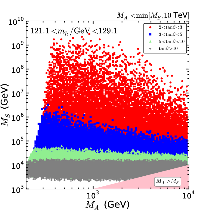
Figure 1: The scatter plot on the ($M_{A}$, $M_{S}$) plane varying input parameters as in Table 2 while requiring $m_{h}$ to be in the $2$-$\sigma$ range: $121.1<m_{h}/\,\mathrm{GeV}<129.1$. The color scheme are: $2<\tan\beta<3$ (red circle), $3<\tan\beta<5$ (blue square), $5<\tan\beta<10$ (green triangle), and $\tan\beta<10$ (gray cross). In the pink region, $M_{A}>M_{S}$ which is out of our current consideration.

We are taking both the PL and MP methods and make comparisons where it is informative. We note that, when we present our result based on the MP method, the systematic uncertainties of the input parameters are automatically included by utilizing a Gaussian prior distribution, see the nuisance parameters in Table 2. On the other hand, when we are using the PL method, the systematic uncertainties are added to the likelihood function.

In Fig. 1 we show the scatter plot on the ($M_{A}$, $M_{S}$) plane by varying input parameters as in Table 2, while requiring $m_{h}$ to be in the $2$-$\sigma$ range: $121.1\,\mathrm{GeV}<m_{h}<129.1\,\mathrm{GeV}$. Different colors represent different $\tan\beta$ ranges. We observe that a larger $M_{S}$ is required for small values of $\tan\beta$ and also as $M_{A}$ decreases. When $\tan\beta\raisebox{-3.69899pt}{~{}\shortstack{$>$ \\ [-0.07cm] $\sim$}}~{}10$, $M_{S}$ becomes almost independent of $M_{A}$ and it lies between $\sim 3$ TeV and $\sim 15$ TeV. When $M_{A}=M_{S}$ is taken as in the scenario B, the value of $M_{S}$ is smaller in order to achieve $m_{h}\sim 125$ GeV. Therefore, in the split-SUSY framework with the intermediate Higgses lighter than $\sim 10$ TeV, $M_{S}$ is generally predicted to be higher especially when $\tan\beta$ is small.

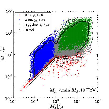
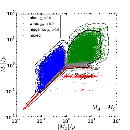
Figure 2: The marginalized posterior (contours) and the profiled likelihood (scatter points) PDFs in the ($|M_{2}|/\mu$, $|M_{1}|/\mu$) plane for the scenarios A (left) and B (right). All the three parameters are the values at the scale $M_{S}$. The inner (outer) contour corresponds to $2\sigma\,(3\sigma)$ credible region (CR) but the scatter points represent the $2\sigma$ profile likelihood region. The regions with $g_{b}>0.9$ (bino-like), $g_{W}>0.9$ (wino-like), and $g_{h}>0.9$ (higgsino-like) are colored in red, blue, and green. The gray region is for the mixed $\chi^{0}_{1}$, see the text.

In Fig. 2 we present the probability density functions (PDFs) for marginalized posterior and profiled likelihood in the ($|M_{2}|/\mu$, $|M_{1}|/\mu$) plane. All the experimental constraints in Table 1 are applied and we make comparisons of the scenarios A (left) and B (right). We represent the bino-like, wino-like, higgsino-like and mixed neutralinos in red, blue, green and gray, respectively. Precisely, we identify the lightest neutralino $\chi^{0}_{1}$ as bino-, wino- or higgsino-like when the corresponding fraction $g_{b}>0.9$, $g_{W}>0.9$ or $g_{h}>0.9$, respectively. Otherwise we identify it is the mixed lightest neutralino. Comparing the scenarios A and B, we can see that the difference lies in the bino region. This is because the bino-like $\chi^{0}_{1}$ can satisfy the relic abundance constraint only through $Z/h$-resonance in the scenario B, where $A/H$-funnel does not work because $M_{A}=M_{S}\raisebox{-3.69899pt}{~{}\shortstack{$>$ \\ [-0.07cm] $\sim$}}~{}3$ TeV. In fact, the mechanism of $Z/h$-resonance requires a small fraction of higgsino but it cannot be too large because of the constraint from the Fermi dSphs gamma ray measurement. In particular, we find that the higgsino composition is between $0.06$ to $0.1$ in the $h$ resonance region which leads to the ratio $|M_{1}|/\mu\sim 0.4$.

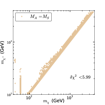
Figure 3: The points with $\delta\chi^{2}<5.99$ scattered on the ($m_{\chi^{0}_{1}}$, $m_{\chi^{\pm}}$) plane for the scenario A (left) and B (right).

Furthermore, we find that the chargino-neutralino coannihilation working in reducing the relic abundance in both scenarios. Being different from the original split SUSY framework (scenario B), one can obtain the correct relic abundance in scenario A without resorting to the coannihilation mechanism thanks to the intermediate Higgses $A$ and $H$. To address this point, we show in Fig. 3 the points with $\delta\chi^{2}<5.99$ on the ($m_{\chi^{0}_{1}}$, $m_{\chi^{\pm}}$) plane for the scenario A (left) and B (right). In addition to the $Z/h$-resonance regions around $m_{\chi^{0}_{1}}\sim 50\,,60$ GeV and the chargino-neutralino coannihilation region along the $m_{\chi^{0}_{1}}=m_{\chi^{\pm}}$ line, we observe there are more points appearing in the scenarios A (left panel) due to the $A/H$-funnel. We find that the $A/H$-funnel region disappears when $m_{\chi^{0}_{1}}>1$ TeV, because the decay widths of $A$ and $H$ become too large and the Breit-Wigner resonance effect is not strong enough to reduce the relic abundance when $M_{H,A}\raisebox{-3.69899pt}{~{}\shortstack{$>$ \\ [-0.07cm] $\sim$}}~{}2$ TeV.

In Fig. 4, we show the marginalized 2D posterior $2$- and $3$-$\sigma$ credible regions (CRs) for the scenario A (left) and B (right) in the ($m_{\chi^{0}_{1}}$, $\langle\sigma v\rangle$) plane. We also show the PL 2-$\sigma$ region (scattered points) for the bino-like (red) and mixed (gray) $\chi^{0}_{1}$ in the upper frames and the wino-like (blue) and higgsino-like (gray) $\chi^{0}_{1}$ in the lower frames. Here $\langle\sigma v\rangle$ denotes the annihilation cross section at the present time which is relevant to the DM indirect detections and through which one may easily identify different mechanisms for the relic abundance.

When $m_{\chi^{0}_{1}}<100\,\mathrm{GeV}$, via the $Z/h$ resonances, the marginalized posterior CRs are located at the bino-like neutralino region with a small amount of higgsino component in both scenarios (see the upper frames). Although the $Z/h$-resonance channels have very good likelihoods, they only fall into the $3\sigma$ (99.73%) CR owing to the small prior volume effect. The similar effect happens for the bino-like $\chi^{0}_{1}$ when $m_{\chi^{0}_{1}}>100$ GeV and the correct relic abundance is obtained by the $\chi\chi^{\pm}$ coannihilation. The fact that more parameter space survives in the scenario A (left) than scenario B (right) is due to the $A/H$-funnel. Nevertheless, most of the additional parameter space is a result of the mixture mechanism between $A/H$-funnel and coannihilation. In the lower frames, we observe that the $2\sigma$ CR has the wino-like branch (blue) with the higher $\langle\sigma v\rangle$ than the higgsino-like one (green). For the wino-like branch, the relic abundance is mainly reduced by the wino-like DM annihilation into $W^{+}W^{-}$ pairs. However when $m_{\chi^{0}_{1}}\raisebox{-3.69899pt}{~{}\shortstack{$>$ \\ [-0.07cm] $\sim$}}~{}3$ TeV, the wino DM cannot give the correct relic abundance as is well known. This mass limit can be slightly extended if coannihilation is taken into account. Since the wino DM have higher annihilation cross sections, the indirect detection constraint is stringent. Indeed, the lower bound for the wino-like neutralino mass is about $300\,\mathrm{GeV}$ from the Fermi dSphs gamma ray constraints. Incidentally, the lower bound for the higgsino-like neutralino mass is about $100\,\mathrm{GeV}$, set by the LEP limit of $m_{\chi_{1}^{\pm}}>103.5$. We further see there is no particular lower bound for the bino-like or mixed neutralino, as seen from the upper frames.

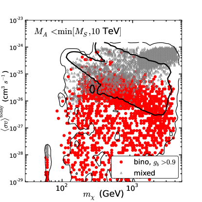
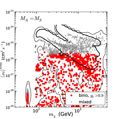
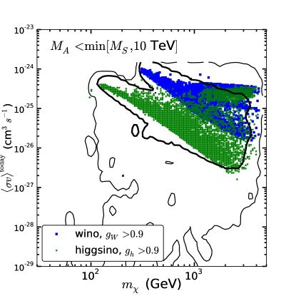
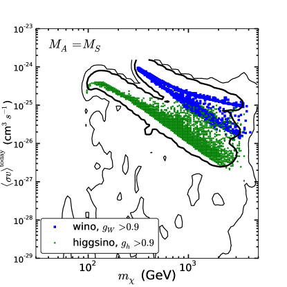
Figure 4: Marginalized posterior PDF (contours) and profiled likelihood PDF (scatter points) in the ($m_{\chi^{0}_{1}}$, $\langle\sigma v\rangle$) plane for the scenario A (left) and B (right). The inner (outer) contours bounded the $2(3)$-$\sigma$ CR. All the scatter points superimposing on the contours agree with likelihood in the criteria $\delta\chi^{2}<5.99$. The red dots, blue squares, green stars, and gray triangle are for the bino-like, wino-like, higgsino-like, and mixed neutralino, respectively.

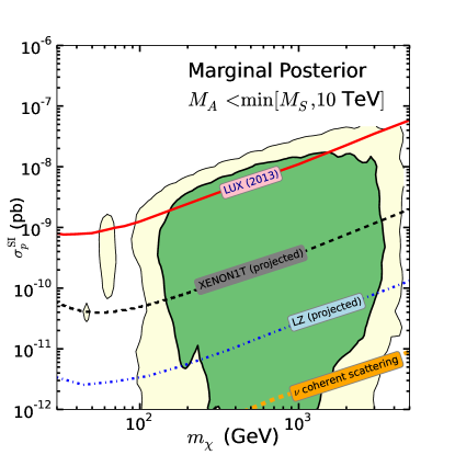
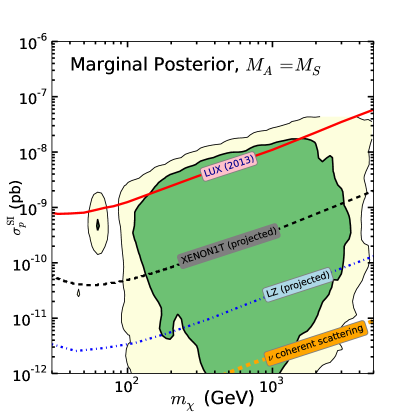
Figure 5: The marginal posterior for the 95% and 99.73% CRs in ($m_{\chi^{0}_{1}}$, $\sigma^{\rm{SI}}_{p}$) plane. The left (right) panel is for the scenario A (B).

Finally, in Fig. 5 we show the marginalized 2D posterior PDF $2\sigma$ and $3\sigma$ contours in the ($m_{\chi^{0}_{1}}$, $\sigma^{\rm{SI}}_{p}$) plane. The red solid line denotes the recent LUX result, the black dashed line the XENON1T projected sensitivity, and the blue dash-dotted line the LZ projected sensitivity [43]. The orange dashed line represents the approximate line below which the DM signal becomes hardly distinguishable from the signals from the coherent scattering of the ${}^{8}B$ solar neutrinos, atmospheric neutrinos and diffuse supernova neutrinos with nuclei. We observe that a part of $2$-$\sigma$ CR is below the LZ projected sensitivity. We can see that, in the $2$-$\sigma$ CRs, there is no significant difference between the scenarios A and B. The $3$-$\sigma$ CRs are slightly different in the lower $\sigma^{\rm{SI}}_{p}$ region. Moreover, in both scenarios, the future 7-tons experiments, LZ, can set a lower limit on the neutralino DM at $m_{\chi^{0}_{1}}>100\,\mathrm{GeV}$.

5 Discussion

In this work, we have studied a “modified split SUSY” scenario, characterized by two separate scales – the SUSY-breaking scale $M_{S}$ and the heavy Higgs-boson mass scale $M_{A}$. This is different from the split SUSY scenario, in which the scale $M_{A}$ is also set at $M_{S}$. The current scenario is motivated by (i) the absence of direct SUSY signals from the searches of scalar quarks up to a few TeV, (ii) the observed Higgs boson is somewhat on the heavy side which needs a large radiative correction to the tree-level mass from heavy stops, and (iii) absence of signals from heavy Higgs bosons $A/H$ and $H^{\pm}$ which can be as light as a few hundred GeV. Therefore, the choice of $M_{A}$ need not be as large as $M_{S}$. We have studied two scenarios: (i) $M_{A}\leq{\rm min}(M_{S},{\rm 10}\,{\rm Tev})$ and (ii) $M_{A}=M_{S}$ (the same as split SUSY).

If both $M_{A}$ and $M_{S}$ are set equal with $M_{A}<10$ TeV, as shown in Fig. 1, only a small region with $M_{S}\raisebox{-3.69899pt}{~{}\shortstack{$<$ \\ [-0.07cm] $\sim$}}~{}10^{4}$ GeV and large $\tan\beta$ is allowed. Nevertheless, if $M_{A}$ and $M_{S}$ are set at different values, much larger parameter space with a wide range of $\tan\beta$ is allowed. With more parameter space we have performed a careful analysis using all dark matter constraints and collider limits.

Because of two distinct scales $M_{S}$ and $M_{A}$ the running of the soft parameters and couplings are separated in two steps. We start with the set of RGEs given in appendix A to run from $M_{S}$ down to $M_{A}$ and perform the matching at the scale $M_{A}$. Then run from $M_{A}$ down to the electro-weakino scale $M_{\chi}\equiv\sqrt{\mu\times M_{2}}$ with the set of RGEs of split SUSY. Because of this two-step RGEs the predictions for DM observables and the Higgs boson mass are more reliable than just a single-step RGE.

We have scanned the MSSM parameter space characterized by the two scales: $M_{S}$ and $M_{A}$ subjected to many existing experimental constraints: invisible widths of the $Z$ boson and the Higgs boson, the chargino mass limit, relic abundance of the LSP, spin-independent cross sections from direct detection, and the gamma-ray data from indirect detection. We found interesting survival regions of parameter space with features of either chargino-neutralino coannihilation, the $A/H$ funnel, or wino-like. These regions survive because of the large enough annihilation to reduce the relic abundance to the observed values, as well as give a large enough Higgs boson mass to fit to the observed value. Finally, the survived parameter space can be further scrutinized by near future direct detection experiments such as XENON1T and LZ.

We offer a few important comments as follows.

1. We used the Higgs boson mass in the range range $121.1<m_{h}<129.1$ GeV to search for suitable $M_{S}$. Since $m_{h}$ is on the rather heavy side, it requires a large radiative correction to the tree-level mass. This can be achieved by a large stop mass and/or large mixing in the stop sector. Since the radiative correction is proportional to some powers of $\tan\beta$, a smaller $\tan\beta$ requires then a larger $M_{S}$ in order to achieve a large enough $m_{h}$. Typically, $M_{S}\raisebox{-3.69899pt}{~{}\shortstack{$>$ \\ [-0.07cm] $\sim$}}~{}10^{5-6}$ GeV for $\tan\beta<3$. For large enough $\tan\beta$ the values of $M_{S}$ is more or less independent of $M_{A}$.

2. On the other hand, if we set $M_{A}=M_{S}$ as we do in scenario A, the allowed $M_{S}$ is rather short from about $10^{3}-10^{4}$ GeV with large $\tan\beta$ (see Fig. 1).

3. An interesting region that satisfies the relic abundance constraint is characterized by nearly degenerate mass among the first two neutralinos and the lightest chargino, indicated by $M_{2}/\mu\approx M_{1}/\mu\approx 1$. The increased effective annihilation cross section can help reducing the relic abundance.

4. Another interesting region is the $Z/h$ resonance region ($m_{\chi^{0}_{1}}\sim 50-60$ GeV), though it is relatively fine-tuned region because of the narrow width of the $Z$ boson and the Higgs boson.

5. Yet, another interesting survival region is the $A/H$ funnel region. If $m_{\chi^{0}_{1}}$ falls around the vicinity of $m_{A/H}/2$ the resonance effect is strong, provided that the width is not too large. This can be achieved for $m_{\chi^{0}_{1}}\raisebox{-3.69899pt}{~{}\shortstack{$<$ \\ [-0.07cm] $\sim$}}~{}1$ TeV, that is $M_{A/H}\raisebox{-3.69899pt}{~{}\shortstack{$<$ \\ [-0.07cm] $\sim$}}~{}2$ TeV. In scenario B, where $M_{S}=M_{A}$, large values of $M_{S}$ then cannot be accepted because the $A/H$ funnel is not working efficiently. However, in scenario A, where $M_{A}<M_{S}$, the $A/H$ funnel can be very effective in reducing the relic abundance, thus more parameter space is allowed.

6. Both wino-like and higgsino-like LSPs have large annihilation cross sections. The allowed mass for $m_{\chi^{0}_{1}}$ ranges from about 300 GeV to 3 TeV for wino-like LSP while from about 100 GeV to 2 TeV for higgsino-like LSP.

7. The current allowed parameter space has a large region below the current LUX limit $\sigma^{\rm SI}_{p}\raisebox{-3.69899pt}{~{}\shortstack{$<$ \\ [-0.07cm] $\sim$}}~{}10^{-9}$ pb. Although the future XENON1T can improve the limit by an order of magnitude, there is still a sizable region below the XENON1T sensitivity. Yet, there still exist some allowed regions even with the future 7-tons size direct detection experiment LZ. Therefore, this modified split SUSY scenario is hard to be excluded in the future.

8. We have used both the methods of profile likelihood and marginal posterior. Though these two statistical approaches have very different methodology, the resulting 2- and 3-$\sigma$ regions are quite consistent, as shown in the figures.

Appendix A RGEs from $M_{S}$ to $M_{A}$

Here we present the one-loop RGEs governing the running of couplings from the high SUSY scale $M_{S}$ to the intermediate Higgs mass scale $M_{A}$.

We write the RGE for each coupling $g_{i}$ present in the theory, in the $\overline{\rm MS}$ or $\overline{\rm DR}$ scheme (the same up to one-loop level), as

$$\frac{dg_{i}}{d\ln Q}=\frac{\beta_{1}(g_{i})}{(4\pi)^{2}}.$$ (A.1)

The relevant coupling constants $g_{i}$ include the gauge couplings ($g_{s},g,g^{\prime}$), the gaugino couplings ($\tilde{g}_{d}^{\prime},\tilde{g}_{u}^{\prime}$, $\tilde{g}_{d},\tilde{g}_{u}$), the third-generation Yukawa couplings ($y_{t},y_{b},y_{\tau}$), and the Higgs quartic ($\lambda_{1},\lambda_{2},\lambda_{3},\lambda_{4},\lambda_{5},\lambda_{6},\lambda_{7}$).

At one loop the $\beta$ functions of gauge couplings below the SUSY scale are given by

$$\beta_{1}(g_{s})=-5g_{s}^{3},\qquad\qquad\beta_{1}(g)=-1g^{3},\qquad\qquad\beta_{1}(g^{\prime})=\frac{23}{3}g^{\prime 3}.$$ (A.2)

The $\beta$ functions of gauge couplings defined by the fermion-scalar-gaugino interaction below the SUSY scale are given by

$$\beta_{1}\left(\tilde{g}_{u}\right) = \tilde{g}_{u}\left(-\frac{33}{4}g^{2}-\frac{3}{4}g^{\prime 2}+\frac{11}{4}\tilde{g}_{u}^{2}+\frac{1}{2}\tilde{g}_{d}^{2}+\frac{3}{4}\tilde{g}_{u}^{\prime 2}+3y_{t}^{2}\right)$$ (A.3)

$$\beta_{1}\left(\tilde{g}_{d}\right) = \tilde{g}_{d}\left(-\frac{33}{4}g^{2}-\frac{3}{4}g^{\prime 2}+\frac{11}{4}\tilde{g}_{d}^{2}+\frac{1}{2}\tilde{g}_{u}^{2}+\frac{3}{4}\tilde{g}_{d}^{\prime 2}+3y_{b}^{2}+y_{\tau}^{2}\right)$$ (A.4)

$$\beta_{1}\left(\tilde{g}_{u}^{\prime}\right) = \tilde{g}_{u}^{\prime}\left(-\frac{9}{4}g^{2}-\frac{3}{4}g^{\prime 2}+\frac{9}{4}\tilde{g}_{u}^{2}+\frac{5}{4}\tilde{g}_{u}^{\prime 2}+\frac{1}{2}\tilde{g}_{d}^{\prime 2}+3y_{t}^{2}\right)$$ (A.5)

$$\beta_{1}\left(\tilde{g}_{d}^{\prime}\right) = \tilde{g}_{d}^{\prime}\left(-\frac{9}{4}g^{2}-\frac{3}{4}g^{\prime 2}+\frac{9}{4}\tilde{g}_{d}^{2}+\frac{5}{4}\tilde{g}_{d}^{\prime 2}+\frac{1}{2}\tilde{g}_{u}^{\prime 2}+3y_{b}^{2}+y_{\tau}^{2}\right)$$ (A.6)

The $\beta$ functions of 3rd generation Yukawa interactions below the SUSY scale are given by

$$\beta_{1}\left(y_{t}\right) = y_{t}\left(\frac{9}{2}y_{t}^{2}+\frac{1}{2}y_{b}^{2}-8g_{s}^{2}-\frac{9}{4}g^{2}-\frac{17}{12}g^{\prime 2}+\frac{3}{2}\tilde{g}_{u}^{2}+\frac{1}{2}\tilde{g}_{u}^{\prime 2}\right)$$ (A.7)

$$\beta_{1}\left(y_{b}\right) = y_{b}\left(\frac{9}{2}y_{b}^{2}+\frac{1}{2}y_{t}^{2}+y_{\tau}^{2}-8g_{s}^{2}-\frac{9}{4}g^{2}-\frac{5}{12}g^{\prime 2}+\frac{3}{2}\tilde{g}_{d}^{2}+\frac{1}{2}\tilde{g}_{d}^{\prime 2}\right)$$ (A.8)

$$\beta_{1}\left(y_{\tau}\right) = y_{\tau}\left(\frac{5}{2}y_{\tau}^{2}+3y_{b}^{2}-\frac{9}{4}g^{2}-\frac{15}{4}g^{\prime 2}+\frac{3}{2}\tilde{g}_{d}^{2}+\frac{1}{2}\tilde{g}_{d}^{\prime 2}\right)$$ (A.9)

The $\beta$ functions of Higgs quartic couplings defined by Haber and Hempfling [44] are given by

$$\beta_{1}\left(\lambda_{1}\right) = \bigg{(}24\lambda_{1}^{2}+4\lambda_{3}^{2}+4(\lambda_{3}+\lambda_{4})^{2}+4\lambda_{5}^{2}+48\lambda_{6}^{2}$$ (A.10)

$$+\frac{3}{8}\Big{(}2g^{4}+(g^{2}+g^{\prime 2})^{2}\Big{)}-\Big{(}2\tilde{g}_{d}^{4}+\frac{1}{2}(\tilde{g}_{d}^{2}+\tilde{g}_{d}^{\prime 2})^{2}\Big{)}-2N_{c}y_{b}^{4}-2y_{\tau}^{4}$$

$$+4\lambda_{1}\gamma_{d}\bigg{)},$$

$$\beta_{1}\left(\lambda_{2}\right) = \bigg{(}24\lambda_{2}^{2}+4\lambda_{3}^{2}+4(\lambda_{3}+\lambda_{4})^{2}+4\lambda_{5}^{2}+48\lambda_{7}^{2}$$ (A.11)

$$+\frac{3}{8}\Big{(}2g^{4}+(g^{2}+g^{\prime 2})^{2}\Big{)}-\Big{(}2\tilde{g}_{u}^{4}+\frac{1}{2}(\tilde{g}_{u}^{2}+\tilde{g}_{u}^{\prime 2})^{2}\Big{)}-2N_{c}y_{t}^{4}$$

$$+4\lambda_{2}\gamma_{u}\bigg{)},$$

$$\beta_{1}\left(\lambda_{3}\right) = \bigg{(}(\lambda_{1}+\lambda_{2})(3\lambda_{3}+\lambda_{4})+8\lambda_{3}^{2}+4\lambda_{4}^{2}+4\lambda_{5}^{2}+8\lambda_{6}^{2}+8\lambda_{7}^{2}+32\lambda_{6}\lambda_{7}$$ (A.12)

$$+\frac{3}{8}\Big{(}2g^{4}+(g^{2}-g^{\prime 2})^{2}\Big{)}-\Big{(}2\tilde{g}_{u}^{2}\tilde{g}_{d}^{2}+\frac{1}{2}(\tilde{g}_{u}^{2}-\tilde{g}_{u}^{\prime 2})(\tilde{g}_{d}^{2}-\tilde{g}_{d}^{\prime 2})\Big{)}-2N_{c}y_{b}^{2}y_{t}^{2}$$

$$+\lambda_{3}(2\gamma_{d}+2\gamma_{u})\bigg{)},$$

$$\beta_{1}\left(\lambda_{4}\right) = \bigg{(}4\lambda_{4}(\lambda_{1}+\lambda_{2}+4\lambda_{3}+2\lambda_{4})+16\lambda_{5}^{2}+20\lambda_{6}^{2}+20\lambda_{7}^{2}+8\lambda_{6}\lambda_{7}$$ (A.13)

$$+\frac{3}{2}g^{2}g^{\prime 2}+2\tilde{g}_{d}^{2}\tilde{g}_{u}^{2}-\tilde{g}_{d}^{2}\tilde{g}_{u}^{\prime 2}-\tilde{g}_{d}^{\prime 2}\tilde{g}_{u}^{2}+2N_{c}y_{b}^{2}y_{t}^{2}$$

$$+\lambda_{4}(2\gamma_{d}+2\gamma_{u})\bigg{)},$$

$$\beta_{1}\left(\lambda_{5}\right) = \bigg{(}4\lambda_{5}(\lambda_{1}+\lambda_{2}+4\lambda_{3}+6\lambda_{4})+20(\lambda_{6}^{2}+\lambda_{7}^{2})+8\lambda_{6}\lambda_{7}$$ (A.14)

$$+\lambda_{5}(2\gamma_{d}+2\gamma_{u})\bigg{)},$$

$$\beta_{1}\left(\lambda_{6}\right) = \bigg{(}4\lambda_{6}(6\lambda_{1}+3\lambda_{3}+4\lambda_{4}+5\lambda_{5})+4\lambda_{7}(3\lambda_{3}+2\lambda_{4}+\lambda_{5})$$ (A.15)

$$+\lambda_{6}(3\gamma_{d}+\gamma_{u})\bigg{)},$$

$$\beta_{1}\left(\lambda_{7}\right) = \bigg{(}4\lambda_{7}(6\lambda_{2}+3\lambda_{3}+4\lambda_{4}+5\lambda_{5})+4\lambda_{6}(3\lambda_{3}+2\lambda_{4}+\lambda_{5})$$ (A.16)

$$+\lambda_{7}(\gamma_{d}+3\gamma_{u})\bigg{)},$$

where

$$\gamma_{d} = N_{c}y_{b}^{2}+y_{\tau}^{2}-\frac{3}{4}(3g^{2}+g^{\prime 2})+\frac{1}{2}(3\tilde{g}_{d}^{2}+\tilde{g}_{d}^{\prime 2}),$$ (A.17)

$$\gamma_{u} = N_{c}y_{t}^{2}-\frac{3}{4}(3g^{2}+g^{\prime 2})+\frac{1}{2}(3\tilde{g}_{u}^{2}+\tilde{g}_{u}^{\prime 2}).$$ (A.18)

The $\beta$ functions of gaugino mass parameters and the SUSY $\mu$ term are given by

$$\beta_{1}\left(M_{3}\right) = -18g_{s}^{2}M_{3}$$ (A.19)

$$\beta_{1}\left(M_{2}\right) = (-12g^{2}+\tilde{g}_{u}^{2}+\tilde{g}_{d}^{2})M_{2}$$ (A.20)

$$\beta_{1}\left(M_{1}\right) = (\tilde{g}_{u}^{\prime 2}+\tilde{g}_{d}^{\prime 2})M_{1}$$ (A.21)

$$\beta_{1}\left(\mu\right) = \left(-\frac{9}{2}g^{2}+\frac{3}{4}\tilde{g}_{u}^{2}+\frac{3}{4}\tilde{g}_{d}^{2}-\frac{3}{2}g^{\prime 2}+\frac{1}{4}\tilde{g}_{u}^{\prime 2}+\frac{1}{4}\tilde{g}_{d}^{\prime 2}\right)\mu$$ (A.22)

Appendix B The statistical framework

To calculate the probability of MSSM parameter given the experimental data, one can employ Bayes’s’ theorem to compute the posterior probability density function,

$$p(\theta,\phi|d)=\frac{\mathcal{L}(d|\theta,\phi)\pi(\theta,\phi)}{\mathcal{Z}(d)}.$$ (B.1)

Here, we denote the MSSM parameters and DM direct detection nuisance parameters as $\theta$ and $\phi$, respectively. The likelihood $\mathcal{L}(d|\theta,\phi)$ is the probability of obtaining experimental data for observables given the MSSM parameters. The prior knowledge of MSSM parameter space is presented as prior distribution $\pi(\theta,\phi)$. Our MSSM prior ranges and distributions are tabulated in Table 2. Finally, the evidence of the model in the denominator can be merely a normalization factor, because we are not interested in model comparison.

The Bayesian approach allows us to simply get ride of the unwanted parameters by using marginalization. For example, if there would be $n$ free model parameters, $r_{i=1,...,n}$, but one is only interesting in the two-dimensional figure ($r_{1}$, $r_{2}$), the marginalization can be written as

$$p(r_{1},r_{2}|d)=\int p(r_{1},...,r_{n}|d)\prod_{i=3}^{n}dr_{i}.$$ (B.2)

An analogous procedure can be performed with the observables. One should keep in mind that a poor prior knowledge or likelihood function can raise a volume effect. In other words, some regions gain more weight from higher prior probability but fine-tuning regions such as resonance regions for relic abundance likelihood only have lower prior probability. Although this is the feature of Bayesian statistics, in order to manifest these fine-tuning regions, we still present both profile likelihood and marginal posterior method at the same time.

In Bayesian statistics, a credible region (CR) is the smallest region, $\mathcal{R}$, in the best agreement with experiments bounded with the fraction $\varrho$ of the total probabilities. For example at MSSM ($M_{1}$, $M_{2}$) plane, the $\varrho$ credible region can be written as

$$\frac{\int_{\mathcal{R}}p(M_{1},M_{2}|d)dM_{1}dM_{2}}{\rm{normalization}}=\varrho,$$ (B.3)

where the normalization in the denominator is the total probability with $\mathcal{R}\to\infty$. In this paper, we have shown $\varrho=0.95$ and $\varrho=0.9973$ corresponding to $2\sigma$ and $3\sigma$ credible region. As the comparison, we also present the scatter points with selected criteria $\delta\chi^{2}=-2\ln\mathcal{L/L_{\rm{max}}}\leq 5.99$. This criteria is $2\sigma$ confidence region of Profile Likelihood method in 2 degrees of freedom. We can see from our result that most of $2\sigma$ confidence region of PL method is similar to the 3 $\sigma$ credible region in MP method. We would like to note that the total profile likelihood here takes the likelihoods including the nuisance parameters distribution, which is the prior distribution in marginal posterior method.

References

- [1] Talk by Monica D’Onofrio (ATLAS Coll.) at SUSY 2014, Manchester, July 2014; talk by Henning Flaecher (CMS Coll.) at SUSY 2014, Manchester, July 2014.
- [2] F. Gabbiani, E. Gabrielli, A. Masiero and L. Silvestrini, Nucl. Phys. B 477, 321 (1996) [hep-ph/9604387]. T. Moroi and M. Nagai, Phys. Lett. B 723, 107 (2013) [arXiv:1303.0668 [hep-ph]]. D. McKeen, M. Pospelov and A. Ritz, Phys. Rev. D 87, no. 11, 113002 (2013) [arXiv:1303.1172 [hep-ph]]. R. Sato, S. Shirai and K. Tobioka, JHEP 1310, 157 (2013) [arXiv:1307.7144 [hep-ph]]. W. Altmannshofer, R. Harnik and J. Zupan, JHEP 1311, 202 (2013) [arXiv:1308.3653 [hep-ph]]. K. Fuyuto, J. Hisano, N. Nagata and K. Tsumura, JHEP 1312, 010 (2013) [arXiv:1308.6493 [hep-ph]].
- [3] S. Weinberg, Phys. Rev. Lett. 48, 1303 (1982). M. Kawasaki, K. Kohri, T. Moroi and A. Yotsuyanagi, Phys. Rev. D 78, 065011 (2008) [arXiv:0804.3745 [hep-ph]]. L. J. Hall and Y. Nomura, JHEP 1201, 082 (2012) [arXiv:1111.4519 [hep-ph]].
- [4] T. Moroi and L. Randall, Nucl. Phys. B 570, 455 (2000) [hep-ph/9906527]. A. Masiero, S. Profumo and P. Ullio, Nucl. Phys. B 712, 86 (2005) [hep-ph/0412058]. K. Cheung, C. W. Chiang and J. Song, JHEP 0604, 047 (2006) [hep-ph/0512192]. F. Wang, W. Wang and J. M. Yang, Phys. Rev. D 72, 077701 (2005) [hep-ph/0507172]. A. Provenza, M. Quiros and P. Ullio, JCAP 0612, 007 (2006) [hep-ph/0609059]. N. Bernal, JCAP 0908, 022 (2009) [arXiv:0905.4239 [hep-ph]]. G. Elor, H. S. Goh, L. J. Hall, P. Kumar and Y. Nomura, Phys. Rev. D 81, 095003 (2010) [arXiv:0912.3942 [hep-ph]]. J. Hisano, K. Ishiwata and N. Nagata, Phys. Lett. B 690, 311 (2010) [arXiv:1004.4090 [hep-ph]]. M. Ibe and T. T. Yanagida, Phys. Lett. B 709, 374 (2012) [arXiv:1112.2462 [hep-ph]]. M. Ibe, S. Matsumoto and T. T. Yanagida, Phys. Rev. D 85, 095011 (2012) [arXiv:1202.2253 [hep-ph]]. L. J. Hall, Y. Nomura and S. Shirai, JHEP 1301, 036 (2013) [arXiv:1210.2395 [hep-ph]]. J. Hisano, K. Ishiwata and N. Nagata, Phys. Rev. D 87, 035020 (2013) [arXiv:1210.5985 [hep-ph]]. M. Ibe, S. Matsumoto, S. Shirai and T. T. Yanagida, JHEP 1307, 063 (2013) [arXiv:1305.0084 [hep-ph]]. M. Ibe, S. Matsumoto, S. Shirai and T. T. Yanagida, arXiv:1409.6920 [hep-ph]. N. Nagata and S. Shirai, arXiv:1410.4549 [hep-ph].
- [5] “Search for Neutral MSSM Higgs bosons in TeV pp collisions at ATLAS”, ATLAS Collaboration, ATLAS-CONF-2012-094; V. Khachatryan et al. [CMS Collaboration], JHEP 1410 (2014) 160 [arXiv:1408.3316 [hep-ex]].
- [6] G. Aad et al. [ATLAS Collaboration], JHEP 1409, 176 (2014) [arXiv:1405.7875 [hep-ex]].
- [7] G. Aad et al. [ATLAS Collaboration], Phys. Lett. B 716, 1 (2012) [arXiv:1207.7214 [hep-ex]]; S. Chatrchyan et al. [CMS Collaboration], Phys. Lett. B 716, 30 (2012) [arXiv:1207.7235 [hep-ex]].
- [8] N. Arkani-Hamed and S. Dimopoulos, JHEP 0506, 073 (2005) [hep-th/0405159]; G. F. Giudice and A. Romanino, Nucl. Phys. B 699, 65 (2004) [Erratum-ibid. B 706, 65 (2005)] [hep-ph/0406088]. N. Arkani-Hamed, S. Dimopoulos, G. F. Giudice and A. Romanino, Nucl. Phys. B 709, 3 (2005) [hep-ph/0409232].
- [9] G. F. Giudice and A. Strumia, “Probing High-Scale and Split Supersymmetry with Higgs Mass Measurements,” Nucl. Phys. B 858 (2012) 63 [arXiv:1108.6077 [hep-ph]].
- [10] J. Beringer et al. [Particle Data Group Collaboration], Phys. Rev. D 86, 010001 (2012).
- [11] K. Cheung, J. S. Lee and P. Y. Tseng, JHEP 1305, 134 (2013) [arXiv:1302.3794 [hep-ph]]; K. Cheung, J. S. Lee and P. Y. Tseng, arXiv:1407.8236 [hep-ph].
- [12] LEP2 SUSY Working Group, http://lepsusy.web.cern.ch/lepsusy/
- [13] P. A. R. Ade et al. [Planck Collaboration], Astron. Astrophys. (2014) [arXiv:1303.5076 [astro-ph.CO]].
- [14] S. Matsumoto, S. Mukhopadhyay and Y. L. S. Tsai, arXiv:1407.1859 [hep-ph].
- [15] D. S. Akerib et al. [LUX Collaboration], Phys. Rev. Lett. 112, 091303 (2014) [arXiv:1310.8214 [astro-ph.CO]].
- [16] Y. L. S. Tsai, Q. Yuan and X. Huang, JCAP 1303, 018 (2013) [arXiv:1212.3990 [astro-ph.HE]].
- [17] M. Ackermann et al. [Fermi-LAT Collaboration], Phys. Rev. D 89, no. 4, 042001 (2014) [arXiv:1310.0828 [astro-ph.HE]].
- [18] M. Ackermann et al. [Fermi-LAT Collaboration], Phys. Rev. D 88, 082002 (2013) [arXiv:1305.5597 [astro-ph.HE]].
- [19] See, for example, talks of F. Frensch (CMS) and M. Zur Nedden (ATLAS), 25th July 2014, in SUSY 2014.
- [20] S. Chatrchyan et al. [CMS Collaboration], JHEP 1211 (2012) 147 [arXiv:1209.6620 [hep-ex]].
- [21] C. Han, arXiv:1409.7000 [hep-ph].
- [22] K. Choi, K. S. Jeong and K. i. Okumura, JHEP 0509, 039 (2005) [hep-ph/0504037].
- [23] J. P. Conlon and F. Quevedo, JHEP 0606, 029 (2006) [hep-th/0605141].
- [24] J. P. Conlon, S. S. Abdussalam, F. Quevedo and K. Suruliz, JHEP 0701, 032 (2007) [hep-th/0610129].
- [25] B. S. Acharya, K. Bobkov, G. L. Kane, P. Kumar and J. Shao, Phys. Rev. D 76, 126010 (2007) [hep-th/0701034].
- [26] B. S. Acharya, K. Bobkov, G. L. Kane, J. Shao and P. Kumar, Phys. Rev. D 78, 065038 (2008) [arXiv:0801.0478 [hep-ph]].
- [27] J. Fan and M. Reece, JHEP 1310, 124 (2013) [arXiv:1307.4400 [hep-ph]].
- [28] N. Blinov, J. Kozaczuk, A. Menon and D. E. Morrissey, arXiv:1409.1222 [hep-ph].
- [29] J. Hisano, S. Matsumoto, M. Nagai, O. Saito and M. Senami, Phys. Lett. B 646, 34 (2007) [hep-ph/0610249].
- [30] S. Mohanty, S. Rao and D. P. Roy, Int. J. Mod. Phys. A 27, no. 6, 1250025 (2012) [arXiv:1009.5058 [hep-ph]].
- [31] R. Catena and P. Ullio, JCAP 1205, 005 (2012) [arXiv:1111.3556 [astro-ph.CO]].
- [32] G. D. Martinez, J. S. Bullock, M. Kaplinghat, L. E. Strigari and R. Trotta, JCAP 0906, 014 (2009) [arXiv:0902.4715 [astro-ph.HE]].
- [33] N. Bernal, A. Djouadi and P. Slavich, JHEP 0707, 016 (2007) [arXiv:0705.1496 [hep-ph]].
- [34] P. Gondolo, J. Edsjo, P. Ullio, L. Bergstrom, M. Schelke and E. A. Baltz, JCAP 0407, 008 (2004) [astro-ph/0406204].
- [35] F. Feroz, M. P. Hobson and M. Bridges, arXiv:0809.3437 [astro-ph].
- [36] G. Aad et al. [ATLAS Collaboration], Phys. Rev. D 90, 052004 (2014) [arXiv:1406.3827 [hep-ex]].
- [37] V. Khachatryan et al. [CMS Collaboration], Eur. Phys. J. C 74, no. 10, 3076 (2014) [arXiv:1407.0558 [hep-ex]].
- [38] L. Alvarez-Ruso, T. Ledwig, J. Martin Camalich and M. J. Vicente-Vacas, Phys. Rev. D 88, no. 5, 054507 (2013) [arXiv:1304.0483 [hep-ph]].
- [39] P. Junnarkar and A. Walker-Loud, Phys. Rev. D 87, no. 11, 114510 (2013) [arXiv:1301.1114 [hep-lat]].
- [40] G. Aad et al. [ATLAS Collaboration], arXiv:1408.7084 [hep-ex].
- [41] Plenary talk by A. David , “Physcis of the Brout-Englert-Higgs boson in CMS”, ICHEP 2014, Spain.
- [42] S. Heinemeyer, O. Stal and G. Weiglein, Phys. Lett. B 710, 201 (2012) [arXiv:1112.3026 [hep-ph]].
- [43] D. C. Malling, D. S. Akerib, H. M. Araujo, X. Bai, S. Bedikian, E. Bernard, A. Bernstein and A. Bradley et al., arXiv:1110.0103 [astro-ph.IM].
- [44] H. E. Haber and R. Hempfling, “The Renormalization group improved Higgs sector of the minimal supersymmetric model,” Phys. Rev. D 48, 4280 (1993) [hep-ph/9307201].